Neural Preset for Color Style Transfer

Zhanghan Ke Affiliation: City University of Hong Kong Yuhao Liu Affiliation: City University of Hong Kong Lei Zhu Affiliation: City University of Hong Kong Nanxuan Zhao Affiliation: Adobe ResearchProject Page: https://zhkkke.github.io/NeuralPreset Rynson W.H. Lau Affiliation: City University of Hong Kong

Abstract

In this paper, we present a Neural Preset technique to address the limitations of existing color style transfer methods, including visual artifacts, vast memory requirement, and slow style switching speed. Our method is based on two core designs. First, we propose Deterministic Neural Color Mapping (DNCM) to consistently operate on each pixel via an image-adaptive color mapping matrix, avoiding artifacts and supporting high-resolution inputs with a small memory footprint. Second, we develop a two-stage pipeline by dividing the task into color normalization and stylization, which allows efficient style switching by extracting color styles as presets and reusing them on normalized input images. Due to the unavailability of pairwise datasets, we describe how to train Neural Preset via a self-supervised strategy. Various advantages of Neural Preset over existing methods are demonstrated through comprehensive evaluations. Besides, we show that our trained model can naturally support multiple applications without fine-tuning, including low-light image enhancement, underwater image correction, image dehazing, and image harmonization.

Figure 1: Our Color Style Transfer Results. (a) State-of-the-art methods PhotoNAS an2019ultrafast and PhotoWCT² PhotoWCT2 produce distort textures (e.g., text in green box) and dissonant colors (e.g., content in orange box). Besides, they have long inference time even on the latest Nvidia RTX3090 GPU (red numbers in brackets). In contrast, our method avoids artifacts and is

\sim

28\times

faster. (b) Our method can produce faithful results on 8K images, but both PhotoNAS and PhotoWCT² run into the out-of-memory problem. Zoom in for better visualization.

1 Introduction

With the popularity of social media (e.g., Instagram and Facebook), people are increasingly willing to share photos in public. Before sharing, color retouching becomes an indispensable operation to help express the story captured in images more vividly and leave a good first impression. Photo editing tools usually provide color style presets, such as image filters or Look-Up Tables (LUTs), to help users explore efficiently. However, these filters/LUTs are handcrafted with pre-defined parameters, and are not able to generate consistent color styles for images with diverse appearances. Therefore, careful adjustments by the users is still necessary. To address this problem, color style transfer techniques have been introduced to automatically map the color style from a well-retouched image (i.e., the style image) to another (i.e., the input image).

Earlier color style transfer methods ColorTransfer; TransColorToGrey; Piti2005NdimensionalPD; Piti2007AutomatedCG focus on retouching the input image according to low-level feature statistics of the style image. They disregard high-level information, resulting in unexpected changes in image inherent colors. Although recent deep learning based models DPST; PhotoWCT; WCT2; an2019ultrafast; DeepPreset; PhotoWCT2 give promising results, they typically suffer from three obvious limitations in practice (Fig. 1 (a)). First, they produce unrealistic artifacts (e.g., distorted textures or inharmonious colors) in the stylized image since they perform color mapping based on convolutional models, which operate on image patches and may have inconsistent outputs for pixels with the same value. Although some auxiliary constraints DPST or post-processing strategies PhotoWCT have been proposed, they still fail to prevent artifacts robustly. Second, they cannot handle high-resolution (e.g., 8K) images due to their huge runtime memory footprint. Even using a GPU with 24GB of memory, most recent models suffer from the out-of-memory problem when processing 4K images. Third, they are inefficient in switching styles because they carry out color style transfer as a single-stage process, requiring to run the whole model every time.

In this work, we present a Neural Preset technique with two core designs to overcome the above limitations:

(1) Neural Preset leverages Deterministic Neural Color Mapping (DNCM) as an alternative to the color mapping process based on convolutional models. By multiplying an image-adaptive color mapping matrix, DNCM converts pixels of the same color to a specific color, avoiding unrealistic artifacts effectively. Besides, DNCM operates on each pixel independently with a small memory footprint, supporting very high-resolution inputs. Unlike adaptive 3D LUTs zeng2020lut; cvpr2022Cong that need to regress tens of thousands of parameters or automatic filters Harmonizer; Exposure that perform particular color mappings, DNCM can model arbitrary color mappings with only a few hundred learnable parameters.

(2) Neural Preset carries out color style transfer in two stages to enable fast style switching. Specifically, the first stage builds a nDNCM from the input image for color normalization, which maps the input image to a normalized color style space representing the “image content”; the second stage builds a sDNCM from the style image for color stylization, which transfers the normalized image to the target color style. Such a design has two advantages in terms of efficiency: the parameters of sDNCM can be stored as color style presets and reused by different input images, while the input image can be stylized by diverse color style presets after normalized once with nDNCM.

In addition, since there are no pairwise datasets available, we propose a new self-supervised strategy for Neural Preset to be trainable. Our comprehensive evaluations demonstrate that Neural Preset outperforms state-of-the-art methods significantly in various aspects. Notably, Neural Preset can produce faithful results for 8K images (Fig. 1 (b)) and can provide consistent color style transfer results across video frames without post-processing. Compared to recent deep learning based models, Neural Preset achieves $\sim$ $28\times$ speedup on a Nvidia RTX3090 GPU, supporting real-time performances at 4K resolution without engineering tricks like model quantization. Finally, we show that our trained model can be applied to other color mapping tasks without fine-tuning, including low-light image enhancement low-light-survey, underwater image correction underwater-survey, image dehazing dehazing-survey, and image harmonization harmonization-survey.

2 Related Works

Color Style Transfer. Unlike artistic style transfer Li2016CombiningMR; Johnson2016Perceptual; d135f1128a; Chen2017StyleBankAE; huang2017adain; Dumoulin2017ALR; deng2021stytr2; DEAIST; Hong_2021_ICCV; Cheng_2021_CVPR; Gatys2016ImageST that alters both textures and colors of images, color style transfer (aka photorealistic style transfer) aims to shift only the colors from one image to another. Traditional methods ColorTransfer; TransColorToGrey; Piti2005NdimensionalPD; Piti2007AutomatedCG mostly match the statistics of low-level features, such as the mean and variance of images ColorTransfer or the histograms of filter responses Piti2005NdimensionalPD. However, these methods often transfer unwanted colors if the style and input images have large appearance differences. Recently, many methods exploiting convolutional neural networks (CNNs) DPST; PhotoWCT; WCT2; an2019ultrafast; DeepPreset; PhotoWCT2 are proposed for color style transfer. For example, Yoo et al. WCT2 introduce a model with wavelet pooling/unpooling to reduce distortions. An et al. an2019ultrafast use network architecture search to explore a more effective asymmetric model. Chiu et al. PhotoWCT2 propose to obtain a more compact model by block-wise training with a coarse-to-fine transformation. To address the limitations (i.e., visual artifacts, huge memory consumption, and inefficient in switching styles) of the aforementioned methods as stated in Sec. 1, we present Neural Preset that supports artifact-free color style transfer with only a small memory footprint, via DNCM, and enables fast style switching, via a two-stage pipeline.

Deterministic Color Mapping with CNNs. Filters and LUTs avoid artifacts as they perform deterministic color mapping to produce consistent outputs for the same input pixel values. Some recent image enhancement and harmonization methods zeng2020lut; cvpr2022Cong; Harmonizer; Exposure have attempted to implement color mapping using filters/LUTs with image-adaptive parameters predicted by CNNs. However, combining filters/LUTs with CNNs for color mapping has clear drawbacks. Filter-based methods Harmonizer; Exposure integrate a finite number of image filters, and can only handle basic color adjustments, e.g., brightness and contrast. LUT-based methods zeng2020lut; cvpr2022Cong need to predict coefficients to linearly merge several template LUTs, because LUTs have a large number of learnable parameters that are difficult to optimize via CNNs. Although the affine bilateral grid hdrnet may model complex color mapping with fewer learnable parameters, it cannot provide deterministic color mapping. Applying it to color style transfer JBL may lead to inharmonious colors in different regions of the image. Instead of adopting the aforementioned schemes, we propose DNCM that has only a few hundred learnable parameters but can model arbitrary deterministic color mappings.

Self-Supervised Learning (SSL). SSL has been widely explored for pre-training 7780647; Chen2020GenerativePF; MAASVL; URLPRL; ULVR; LFWOM; MOCO; simclr; BYOL. Some works also solve specific vision tasks via SSL Hoyer2021ThreeWT; Laine2019HighQualitySD; SSH. Since it is expensive to annotate ground truths for color style transfer, most methods either minimize perceptual losses Gatys2016ImageST; Chen2017StyleBankAE; huang2017adain; DPST or match the statistics of image features WCT; PhotoWCT; WCT2; PhotoWCT2. However, such weak constraints usually result in severe visual artifacts. Yim et al. FST and Ho et al. DeepPreset suggest imposing stronger constraints by reconstructing perturbed images, but their trained models can only transfer color styles to images with natural appearances, e.g., images taken by a camera without post-processing. To this end, we present a new SSL strategy for Neural Preset, which not only learns from reconstructing perturbed images but also enables the trained models to transfer color styles between arbitrary images.

3 Method

Our Neural Preset performs color style transfer through a two-stage pipeline, where both stages employ DNCM for color mapping. In this section, we first introduce DNCM in details (Sec. 3.1). We then present the two-stage DNCM-based color style transfer pipeline (Sec. 3.2). Finally, we describe our self-supervised learning strategy for training Neural Preset (Sec. 3.3).

3.1 Deterministic Neural Color Mapping (DNCM)

A straightforward idea to model deterministic color mapping that can adapt to different images is to combine filters/LUTs with the image-adaptive parameters predicted by CNNs. However, each image filter can only provide a single color mapping. Integrating a finite number of filters can only cover a limited range of color mappings. Besides, as a common 32-level 3D LUT has $\sim$ 10K parameters, it is infeasible to regress image-specific 3D LUTs. The approach based on predicting coefficients to merge template LUTs still needs to optimize tens of thousands of parameters to build template LUTs.

Refer to caption — Figure 2: Illustration of DNCM. The DNCM parameters consist of two color projection matrices ( $\mathbf{P}$ , $\mathbf{Q}$ ) and image-adaptive parameters $\mathbf{T}$ predicted by an encoder $E$ . Here, we obtain $\mathbf{\tilde{I}}$ by downsampling $\mathbf{I}$ . DNCM maps the input image $\mathbf{I}$ to output image $\mathbf{Y}$ by multiplying $\mathbf{I}$ with $\mathbf{P}$ , $\mathbf{T}$ , and $\mathbf{Q}$ sequentially.

Here, we propose DNCM to model arbitrary deterministic color mapping with much fewer learnable parameters. As shown in Fig. 2, given an input image $\mathbf{I}$ of size $(h,w,3)$ , we downsample it to obtain a thumbnail $\mathbf{\tilde{I}}$ , which provides image-adaptive color mapping matrix $\mathbf{T}$ for DNCM. Specifically, we feed $\mathbf{\tilde{I}}$ into an encoder $E$ to predict $\mathbf{T}$ of size $(k\times k)$ , and then reshape it to a size of $(k,k)$ , as:

\mathbf{T}^{(k\times k)}=E(\,\mathbf{\tilde{I}}\,),\;\;\mathbf{T}^{(k\times k)}\rightarrow\mathbf{T}^{(k,k)},

(1)

where $\rightarrow$ denotes the reshape operation, and $k$ is empirically set to a small value (e.g., 16). With matrix $\mathbf{T}^{(k,k)}$ , we form DNCM to alter the colors of $\mathbf{I}$ . In DNCM, we first unfold $\mathbf{I}$ as a 2D matrix of size $(h\times w,3)$ . We then embed each pixel in $\mathbf{I}$ into a k-dimensional vector by a projection matrix $\mathbf{P}^{(3,k)}$ . After that, we multiply the embedded vectors by $\mathbf{T}^{(k,k)}$ . Finally, we apply another projection matrix $\mathbf{Q}^{(k,3)}$ to convert the embedded vectors back to the RGB color space and reshape pixels to output $\mathbf{Y}$ with new colors. Note that both $\mathbf{P}$ and $\mathbf{Q}$ are learnable matrices shared by all images. Formally, DNCM can be defined as:

\mathbf{Y}=\textit{DNCM}(\mathbf{I},\,\mathbf{T})=\mathbf{I}^{(h\times w,3)}\cdot\mathbf{P}^{(3,k)}\cdot\mathbf{T}^{(k,k)}\cdot\mathbf{Q}^{(k,3)},

(2)

where $\cdot$ denotes matrix multiplication. We omit the reshape operations in Eq. 2 for simplicity. Note that $\mathbf{Q}$ is not the inverse of $\mathbf{P}$ , since $\mathbf{P}$ is not a square matrix when $k\neq 3$ .

Implementing color mapping as Eq. 2 brings three main benefits. First, it effectively avoids visual artifacts as pixels of the same color in $\mathbf{I}$ will still have the same color after being mapped to $\mathbf{Y}$ . Second, it requires only a small memory footprint since each pixel is processed independently with efficient matrix multiplications. Third, it makes $E()$ easy to optimize as only $k\times k$ image-adaptive parameters (i.e., $\mathbf{T}$ ) should be regressed.

3.2 Two-Stage Color Style Transfer Pipeline

Recent methods implicitly embed the color style transfer process into CNNs to form single-stage pipelines. Therefore, they must run the whole pipeline every time to compute the color mapping between two images, which is inefficient when applying diverse color styles to an image or transferring a color style to multiple images.

In contrast, we design an explicit two-stage pipeline based on DNCM. The key insight behind our pipeline is that if we can separate the color style of an image from its “image content”, we can effectively transfer different color styles to the “image content”. However, to achieve this, we need to answer two questions. First, how to remove or add color styles? Since we need to alter the image color style but preserve the “image content”, we propose to utilize a pair of nDNCM and sDNCM. While nDNCM converts the input image to a space that contains only the “image content”, sDNCM transfers the “image content” to the target color style, using parameters extracted from the style image. Second, how to represent “image content”? Since this concept is difficult to define through hand-crafted features, we propose to learn a normalized color style space representing the “image content” by back-propagation. In such a normalized color style space, images of the same content but with different color styles should have a consistent appearance, i.e., the same normalized color style.

As shown in Fig. 3 (a)(b), we modify the encoder $E$ to output $\mathbf{d}$ and $\mathbf{r}$ , which are applied as the parameters of nDNCM and sDNCM, respectively. Suppose that we want to transfer the color style of a style image $\mathbf{I}_{s}$ to an input image $\mathbf{I}_{c}$ . In the first stage, we convert $\mathbf{I}_{c}$ to $\mathbf{Z}_{c}$ in the normalized color style space via nDNCM with $\mathbf{d}_{c}$ predicted from $\mathbf{\tilde{I}}_{c}$ , as:

\mathbf{Z}_{c}=\textit{nDNCM}(\mathbf{I}_{c},\,\mathbf{d}_{c}),\;\;\text{where}\;\;\{\mathbf{d}_{c},\mathbf{r}_{c}\}=E(\mathbf{\tilde{I}}_{c}).

(3)

In the second stage, we extract $\mathbf{r}_{s}$ , i.e., the parameters containing the color style of $\mathbf{I}_{s}$ , to transfer $\mathbf{Z}_{c}$ to the stylized image $\mathbf{Y}_{s}$ via sDNCM, as:

\mathbf{Y}_{s}=\textit{sDNCM}(\mathbf{Z}_{c},\,\mathbf{r}_{s}),\;\;\text{where}\;\;\{\mathbf{d}_{s},\mathbf{r}_{s}\}=E(\mathbf{\tilde{I}}_{s}).

(4)

$E()$ used in Eq. 3 and 4 have shared weights. nDNCM and sDNCM have different projection matrices $\mathbf{P}$ and $\mathbf{Q}$ .

By storing color style parameters (e.g., $\mathbf{r}_{s}$ ) as presets and reusing them to construct sDNCM, our pipeline can support fast style switching using color style presets – we only need to normalize the color style of the input image once, and can then quickly retouch it to diverse color styles by sDNCM with the stored presets (e.g., $\mathbf{r}_{s}$ ). For example, in Fig. 3 (c), we apply presets $\mathbf{r}_{1}$ and $\mathbf{r}_{2}$ on $\mathbf{Z}_{c}$ to obtain $\mathbf{Y}_{1}$ and $\mathbf{Y}_{2}$ .

3.3 Self-Supervised Training Strategy

Figure 4: Our Self-Supervised Training Strategy. Both

\mathbf{I}_{i}

\mathbf{I}_{j}

are generated from

\mathbf{I}

via random color perturbations. We constrain

\mathbf{Z}_{i}

\mathbf{Z}_{j}

to be the same via a consistency loss

\mathcal{L}_{con}

and learn style transfer results

\mathbf{Y}_{i}

\mathbf{Y}_{j}

via a reconstruction loss

\mathcal{L}_{rec}

We develop a self-supervised strategy to train Neural Preset, as shown in Fig. 4. Since no ground truth stylized images are available, we create pseudo stylized images from the input image $\mathbf{I}$ . Specifically, we add perturbations on $\mathbf{I}$ to obtain two augmented samples with different color styles, which are denoted as $\mathbf{I}_{i}$ and $\mathbf{I}_{j}$ . The perturbations we use involve operations that only change image colors, e.g., random image filters or LUTs.

The first stage of our pipeline aims to normalize the color style of input images, which means that input images with the same content but different color styles should be consistent in the normalized color style space. Hence, we apply a L2 consistency loss between the outputs of this stage. Formally, we predict the nDNCM parameters $\mathbf{d}_{i}$ / $\mathbf{d}_{j}$ to transfer $\mathbf{I}_{i}$ / $\mathbf{I}_{j}$ to $\mathbf{Z}_{i}$ / $\mathbf{Z}_{j}$ , and we constrain $\mathbf{Z}_{i}$ / $\mathbf{Z}_{j}$ by:

\begin{split}\mathcal{L}_{con}&=||\mathbf{Z}_{i}-\mathbf{Z}_{j}||_{2}\\ &=||\textit{nDNCM}(\mathbf{I}_{i},\,\mathbf{d}_{i})-\textit{nDNCM}(\mathbf{I}_{j},\,\mathbf{d}_{j})||_{2}.\end{split}

(5)

The second stage of our pipeline aims to stylize the normalized images. To convert the input images to new styles, we swap the predicted sDNCM parameters $\mathbf{r}$ to stylize the two samples, i.e., $\mathbf{Z}_{i}$ will be stylized by $\mathbf{r}_{j}$ while $\mathbf{Z}_{j}$ by $\mathbf{r}_{i}$ , as:

\mathbf{Y}_{i}=\textit{sDNCM}(\mathbf{Z}_{j},\,\mathbf{r}_{i}),\quad\mathbf{Y}_{j}=\textit{sDNCM}(\mathbf{Z}_{i},\,\mathbf{r}_{j}).

(6)

We apply a L1 reconstruction loss between $\mathbf{I}$ and $\mathbf{Y}$ to learn color style transfer, as:

\mathcal{L}_{rec}=||\mathbf{Y}_{i}-\mathbf{I}_{i}||_{1}+||\mathbf{Y}_{j}-\mathbf{I}_{j}||_{1}.

(7)

The final loss is a combination of Eq. 5 and 7, as:

\mathcal{L}=\mathcal{L}_{rec}+\lambda\,\mathcal{L}_{con},

(8)

where $\lambda$ is a controllable weight. Refer to the analysis in Appendix A on how to derive our training constraints from the fundamental color style transfer objective.

4 Experiments

In this section, we first introduce our experimental setting, including datasets, implementation, and quantitative metrics. We then extensively compare Neural Preset with existing color style transfer methods (Sec. 4.1). We further analyze the components and hyper-parameters of Neural Preset through ablation experiments (Sec. 4.2).

Datasets. Following recent color style transfer methods WCT2; an2019ultrafast; PhotoWCT, we train our model on the images from the MS COCO MSCOCO dataset. We use about 5,000 LUT files, along with the random image filter adjustment strategy Harmonizer, as input color perturbations during training. We collect 50 images with diverse color styles and pair each two of them to build a validation set consisting of 2,500 samples.

Implementation. We adopt EfficientNet-B0 EfficientNet as the encoder $E$ in Neural Preset. We fix the input size of $E$ to $256\times 256$ . We set the parameter dimension $k$ in DNCM to $16$ , so the number of parameters predicted by $E$ is only $256$ for each image. We train Neural Preset by the Adam Adam optimizer for $32$ epochs. With a batch size of $24$ , the initial learning rate is $3e^{-4}$ and is multiplied by $0.1$ after $24$ epochs. We set the loss weight $\lambda$ to $10$ .

Method	CT ColorTransfer	PhotoWCT PhotoWCT	WCT² WCT2	PhotoNAS an2019ultrafast	PhotoWCT² PhotoWCT2	Deep Preset DeepPreset	Ours
Average Ranking $\downarrow$	4.97	5.75	2.67	3.39	4.11	5.30	1.81

Table 1: Average Ranking of Different Methods in the User Study. The lower the number, the better the human subjective evaluation.

Quantitative Metrics. We follow prior works WCT2; an2019ultrafast; JBL to quantitatively evaluate color style transfer quality in terms of style similarity (between the output and the reference style image) and content similarity (between the output and the input image). However, we observe from our experiments that the metrics used by prior works cannot reflect color style transfer quality precisely. Therefore, we propose improved style/content similarity measures as our quantitative metrics. For style similarity measure, prior works use the VGG VGG features learned from ImageNet ImageNet to compute the Gram metric. Since the VGG features are not designed for comparing color styles and contain semantic information, the style similarity that they produce may not be accurate due to semantic bias. Instead, we train a discriminator GAN model on an annotated dataset (containing 700 + color style categories, each with 6-10 images of the same color style retouched by human experts) to accurately predict the color style similarity score (in $[0,1]$ ) of two images. For content similarity measure, prior works compute the SSIM metric based on image edges extracted by an edge detection model HED HN_Edge. However, HED only predicts rough edges and is often incorrect. Hence, we replace HED with a recent model LDC xsoria2022ldc, which can output fine and correct edges for SSIM calculation, providing a reliable content similarity score (in $[0,1]$ ). Refer to Appendix B for more details on our improved metrics.

4.1 Comparisons

We compare Neural Preset with deep learning based methods (PhotoWCT PhotoWCT, WCT² WCT2, PhotoNAS an2019ultrafast, PhotoWCT² PhotoWCT2, and Deep Preset DeepPreset) as well as a traditional method (CT ColorTransfer). We evaluate the pre-trained models released by their authors. We do not compare with methods whose codes, models, and demos are all unavailable.

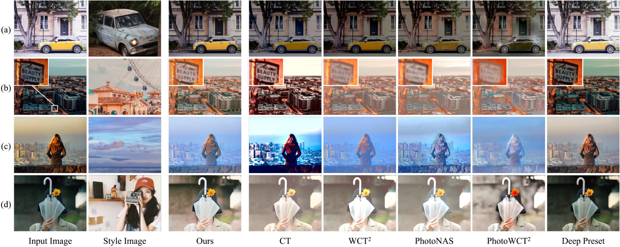
Qualitative Results. Fig. 5 shows the superiority of our qualitative results. First, Neural Preset produces more natural stylized images (e.g., the colors of the car and wall in Fig. 5 (a)). Second, Neural Preset can preserve fine textures with target color styles (e.g., the enlarged text in Fig. 5 (b)). Third, Neural Preset is better at maintaining the inherent object colors (e.g., the human hair and clothing regions in Fig. 5 (c)). Fourth, the outputs of Neural Preset have more consistent color properties with the style images (e.g., the brightness and contrast in Fig. 5 (d)). The results of PhotoWCT are omitted in Fig. 5 as its visual results are similar to PhotoWCT². Refer to Appendix C.1 for more visual results of Neural Preset. Refer to Appendix C.2 for video stylization results of Neural Preset.

Quantitative Results. Fig. 6 shows that our Neural Preset comes closest to the “Ideal” stylization quality. Although PhotoWCT² has high style similarity scores in Fig. 6, we can observe from Fig. 5 that it tends to overfit the color styles of the reference images, which however leads to worse visual results. Deep Preset has high content similarity scores in Fig. 6 since it often fails to alter the color style of input images, as shown in Fig. 5. Besides, both scores for CT are low as it sometimes produces very erratic results.

Figure 6: Quantitative Comparison. The higher the content similarity and the style similarity, the better the stylization quality. “Ideal” refers to the best possible quality. The points on the blue dashed curve have equal distance from “Ideal” as our method, i.e., have equivalent color style transfer quality as our method.

Method	GPU Inference Time $\downarrow$ / Memory $\downarrow$				Model Size $\downarrow$
Method	FHD (1920 $\times$ 1080)	2K (2560 $\times$ 1440)	4K (3840 $\times$ 2160)	8K (7680 $\times$ 4320)	Number of Parameters
PhotoWCT PhotoWCT	0.599 s / 10.00 GB	1.002 s / 16.41 GB	OOM	OOM	8.35 M
WCT² WCT2	0.557 s / 18.75 GB	OOM	OOM	OOM	10.12 M
PhotoNAS an2019ultrafast	0.580 s / 15.60 GB	0.988 s / 23.87 GB	OOM	OOM	40.24 M
Deep Preset DeepPreset	0.344 s / 8.81 GB	0.459 s / 13.21 GB	1.128 s / 22.68 GB	OOM	267.77 M
PhotoWCT² PhotoWCT2	0.291 s / 14.09 GB	0.447 s / 19.75 GB	1.036 s / 23.79 GB	OOM	7.05 M
Ours	0.013 s / 1.96 GB	0.016 s / 1.96 GB	0.019 s / 1.96 GB	0.061 s / 1.96 GB	5.15 M

Table 2: Comparison on GPU Inference Time / Memory, and Model Size. All evaluations are conducted with Float32 model precision on a Nvidia RTX3090 GPU (24GB memory). The values in parentheses under the resolutions are the exact image width and height. The units “s”, “GB”, and “M” mean seconds, gigabytes, and millions, respectively. “OOM” means having the out-of-memory issue.

User Study. We further conduct a user study to evaluate the subjective quality of different methods. We invite 58 users and show them 20 image sets randomly selected from our validation set, with each image set consisting of an input image, a reference style image, and 7 randomly shuffled color style transfer results. For each image set, the users are required to rank the overall stylization quality of the 7 results by considering the style/content similarity and the photorealism of the results as well as whether the color style of the results is visually pleasing. After collected 1,160 (58 $\times$ 20) results, we compute the average ranking of each method. Table 1 shows that results from our method are largely preferred by the users. Note that the second-ranked WCT² can only handle images of FHD resolution (see Table 2). We provide Top1-Top3 ratios Appendix C.4.

Inference Efficiency and Model Size. As shown in Table 2, Neural Preset achieves nearly $28\times$ speedup compared to the fastest state-of-the-art method (i.e., PhotoWCT² PhotoWCT2) on 2K images. Neural Preset also enables real-time inference (about $52$ fps) at 4K resolution, and can handle 8K resolution images at over $16$ fps. Refer to Appendix C.6 for the inference time on CPU. Table 2 also shows that existing methods require large amounts of memory for inference. Using even a GPU with 24GB memory, many of them still have the out-of-memory problem at 4K resolution, and all of them fail at 8K resolution. In contrast, Neural Preset requires only 1.96GB of memory, irrespective of the image resolution. This is because nDNCM/sDNCM in Neural Preset operate on each pixel independently, allowing us to save memory via splitting high-resolution images into small patches for processing. Besides, Neural Preset also has the lowest number of parameters.

Comparing Neural Preset with Filters and Luts. After manually retouching an image by a photo editing tool (e.g., Lightroom), we export the editing parameters as a preset in the filters/LUTs format to process a set of images automatically. Meanwhile, we transfer the color style of the retouched image to other images via Neural Preset. As shown in Fig. 7, filters/LUTs fail to convert images with diverse color styles to a consistent color style (Fig. 7 (b)). For example, after applying filters/LUTs, bright images will be overexposed while dark images still remain dark. In contrast, with the color style parameters extracted from the retouched image, Neural Preset provides results with more consistent color styles (Fig. 7 (c)). Refer to Appendix C.3 for more results of applying the same color style to different input images via Neural Preset.

At 8K Resolution (7680 $\times$ 4320)
Patch Size	Total Patches	GPU Inference Time $\downarrow$ / Memory $\downarrow$
256	507	0.1026 s / 1.83 GB
512	127	0.0613 s / 1.96 GB
1024	32	0.0590 s / 2.14 GB
2048	8	0.0582 s / 2.79 GB
4096	2	0.0575 s / 5.38 GB
8092	1	0.0569 s / 8.77 GB

Table 3: Effects of Different DNCM Input Patch Sizes. We validate the inference time and memory cost of Neural Preset with different DNCM input patch sizes on 8K images. In Table 2, we use a patch size of 512 (the underlined row).

4.2 Ablation Studies

Input Patch Size for DNCM. The input patch size used for DNCM can affect the inference time and memory footprint of Neural Preset. Intuitively, processing a large number of pixels in parallel (i.e., using a larger patch size) will give a lower inference time but at the cost of a higher memory consumption. From Table 3, setting a patch size $>512$ brings a limited speed improvement on a Nvidia RTX3090 GPU but a significant increase in memory usage. This is because the 512 patch size already uses up all GPU cores.

DNCM vs. CNN Color Mapping. We experiment with constructing the proposed two-stage color style transfer pipeline using two CNNs, e.g., two autoencoders UNet, with all other settings unchanged. The results in Fig. 8 visualize our analysis in Appendix A: using DNCM instead of CNN for color mapping prevents our self-supervised training strategy from converging to a trivial solution.

Parameter Dimension $k$ in DNCM. Table 4 shows that setting $k<16$ significantly decreases style similarity but has small effect on content similarity, while setting $k>16$ leads to better performances but also requires longer inference time. Hence, we use $k=16$ , which provides a good balance of speed and performance. Fig. 9 displays the results with different values of $k$ , demonstrating that $k$ also has a huge impact on qualitative results.

$k$	2	4	8	16	32
Style Similarity $\uparrow$	0.128	0.510	0.636	0.746	0.769
Content Similarity $\uparrow$	0.765	0.823	0.781	0.771	0.764

Table 4: Results of Neural Preset with Different Values of

k

. The hyper-parameter

k

has a huge impact on style similarity. Other figures and tables are based on

k=16

(the underlined column).

Effectiveness of $\mathcal{L}_{con}$ . We visualize the “image content” output by the first stage of our pipeline in Fig. 10. Applying $\mathcal{L}_{con}$ provides a more consistent $\mathbf{Z}$ to represent the “image content”. Besides, our experiments also show that learning Neural Preset with $\mathcal{L}_{con}$ can yield better results, i.e., $\mathcal{L}_{con}$ helps the pipeline converge better.

5 Applications

With the proposed self-supervised strategy, Neural Preset is able to learn general knowledge of color style transfer from large-scale data. As a result, given a reference image, our trained model can be naturally applied to other color mapping tasks without fine-tuning. We evaluate four tasks: low-light image enhancement low-light-survey, underwater image correction underwater-survey, image dehazing dehazing-survey, and image harmonization harmonization-survey. These tasks are challenging for universal color style transfer models as the input images typically come from highly degraded domains. The qualitative results in Fig. 11 show that Neural Preset significantly outperforms prior color style transfer methods on all four tasks. We notice that our DNCM effectively avoids heavy visual artifacts produced by other methods, and our color normalization stage successfully decouples color styles from degraded input images. Refer to Appendix C.5 for comparisons with more color style transfer methods on these four tasks.

Besides, training DNCM (Fig. 2) for color mapping tasks using pairwise data is straightforward. We experiment with DNCM on the pairwise datasets of image harmonization DIH; cvpr2022Cong; Harmonizer and image color enhancement hdrnet; zeng2020lut; Exposure. Without whistles and bells, we get top-level performances on both tasks. Refer to Appendix D for details and results.

On-device on_device1 (e.g., mobile or browser) deployment is also vital in practice. It expects a small computational overhead in the client to support real-time UI responses and a small amount of data exchanges between the client/server to save network bandwidth, which are hard to achieve by existing color style transfer models. Instead, Neural Preset enables distributed deployment, which is friendly for on-device applications. Refer to Appendix E for details.

6 Conclusion

In this paper, we have presented a simple but effective Neural Preset technique for color style transfer. Benefited by the proposed DNCM and two-stage pipeline, Neural Preset has shown significant improvements over existing state-of-the-art methods in various aspects. In addition, we have also explored several applications of our method. For example, directly applying Neural Preset to other color mapping tasks without fine-tuning.

Nonetheless, Neural Preset does have limitations. First, if the input is compressed by JPEG with a high compression ratio, the existing JPEG artifacts may be amplified in the output (Fig.12 (a)). Second, it may fail to transfer color styles between images with very different inherent colors (Fig.12 (b)). Third, it cannot perform local-adaptive color mapping to transfer the same color in an image to different colors (Fig.12 (c)). A possible future work is to address these limitations. For example, developing auxiliary regularization to alleviate the effects of JPEG artifacts or incorporating appropriate user interactions for complex cases that involve changing image inherent colors.

Appendices

A Optimization Problem of Neural Preset

Here we analyze (1) how to derive our training constraints from the fundamental color style transfer objective and (2) why performing color mapping via the proposed DNCM is necessary for our training strategy.

Consider the objective of color style transfer. Given an input image $\mathbf{I}_{c}$ and a style image $\mathbf{I}_{s}$ that have different content and color styles, we aim to learn a model $H$ to transfer the color style of $\mathbf{I}_{s}$ to $\mathbf{I}_{c}$ by minimizing the objective:

\min\;\mathbb{E}_{\mathbf{I}_{c},\mathbf{I}_{s},\mathbf{G}_{s}\sim p_{\mathbf{I}}}\big[\,|\mathbf{G}_{s}-H(\mathbf{I}_{c},\mathbf{I}_{s})|\,\big],

(9)

where $p_{\mathbf{I}}$ represents the distribution of images, and $\mathbf{G}_{s}$ is the ground truth stylized image that has the same image content as $\mathbf{I}_{c}$ and the consistent color style as $\mathbf{I}_{s}$ .

The idea of our two-stage pipeline is to divide $H$ into two sub-functions, i.e., two stages, to remove the original image color style of $\mathbf{I}_{c}$ before applying a new one, as:

\min\;\mathbb{E}_{\mathbf{I}_{c},\mathbf{I}_{s},\mathbf{G}_{s}\sim p_{\mathbf{I}}}\big[\,|\mathbf{G}_{s}-S_{2}(S_{1}(\mathbf{I}_{c}),\mathbf{I}_{s})|\,\big],

(10)

where $S_{1}$ and $S_{2}$ denote the sub-functions corresponding to the two stages of our pipeline. As $\mathbf{G}_{s}$ is typically unavailable in practice, we generate pseudo input and style images to approximate the above optimization problem. Specifically, we add random color perturbations (e.g., LUTs or filters) to each image $\mathbf{I}$ to create a set of $n$ images $\{\mathbf{I}_{1},\dots,\mathbf{I}_{n}\}$ with the same content but different color styles. We denote indexes by $i,j\in\{0,\dots,n\}$ in the following context. Thus, Eq. 10 can be approximated with perturbed images, as:

\min\;\mathbb{E}_{\mathbf{I}\sim p_{\mathbf{I}}}\Big[\,\sum_{i}^{n}\sum_{j}^{n}\Big|\mathbf{I}_{j}-S_{2}(S_{1}(\mathbf{I}_{i}),\mathbf{I}_{j})\Big|\,\Big].

(11)

Given any fixed $S_{1}$ , the optimal $S_{2}^{*}$ should satisfy:

\mathbf{I}_{j}=S_{2}^{*}(S_{1}(\mathbf{I}_{j}),\mathbf{I}_{j})=S_{2}^{*}(S_{1}(\mathbf{I}_{i}),\mathbf{I}_{j}).

(12)

Eq. 12 reveals a possible optimization issue of Eq. 11 – if we model $S_{1}$ and $S_{2}$ by end-to-end CNNs like autoencoders UNet, optimizing only Eq. 11 via gradient-based algorithms can easily make $S_{1}$ and $S_{2}$ converge to a trivial solution to satisfy Eq. 12: $S_{2}^{*}$ becomes an identity function w.r.t. $\mathbf{I}_{j}$ , while $S_{1}$ can be any function. Formally, for a real input and style image pair $\mathbf{I}_{c}$ and $\mathbf{I}_{s}$ with different content, the possible trivial solution is:

\mathbf{I}_{s}=S_{2}^{*}(\phi,\mathbf{I}_{s}),\quad\phi:=S_{1}(\mathbf{I}_{c}),

(13)

where $S_{2}^{*}$ always output $\mathbf{I}_{s}$ directly and ignore another input $\phi$ . Such a solution is undesired because the color style transfer objective (Eq. 9) requires the output image have the same content with $\mathbf{I}_{c}$ .

To overcome the above problem, modeling $S_{1}$ and $S_{2}$ via DNCM instead of end-to-end CNNs is necessary. DNCM inputs the color style parameters $E(\mathbf{\tilde{I}}_{j})$ rather than the image $\mathbf{I}_{j}$ . Since the dimensions of $E(\mathbf{\tilde{I}}_{j})$ is much lower than $\mathbf{I}_{j}$ , it prevents $S_{2}$ from being an identity function w.r.t. $\mathbf{I}_{j}$ and forces $S_{1}$ to be involved in computing the optimal solution. Specifically, we define:

\begin{split}S_{1}(\mathbf{I}_{i})&:=\textit{nDNCM}(\mathbf{I}_{i},E(\mathbf{\tilde{I}}_{i})),\\ S_{2}(S_{1}(\mathbf{I}_{i}),\mathbf{I}_{j})&:=\textit{sDNCM}(S_{1}(\mathbf{I}_{i}),E(\mathbf{\tilde{I}}_{j}))).\end{split}

(14)

The formulas/symbols in Eq. 14 are equivalent to those in Sec. 3.2 of the paper. Benefited by DNCM, optimizing only Eq. 11 is sufficient for preventing $S_{1}$ and $S_{2}$ from converging to the trivial solution shown in Eq. 13. There are other possible approaches to avoid such a trivial solution without using DNCM, e.g., modeling the optimization of our pipeline as a bi-level optimization bilevel-survey; bilevel-grad problem.

Let us review Eq. 12 by substituting in Eq. 14, it is obvious that constraining $S_{1}(\mathbf{I}_{i})$ and $S_{1}(\mathbf{I}_{j})$ to be consistent will make $S_{2}^{*}$ easier to obtain. Hence, we interpret Eq. 11 as a constrained optimization problem:

\begin{split}\min\;\mathbb{E}_{\mathbf{I}\sim p_{\mathbf{I}}}\Big[\,\sum_{i}^{n}\sum_{j}^{n}\Big|\mathbf{I}_{j}-S_{2}(S_{1}(\mathbf{I}_{i}),\mathbf{I}_{j})\Big|\,\Big]\\ s.t.\quad\sum_{i}^{n}\sum_{j}^{n}\Big|S_{1}(\mathbf{I}_{j})-S_{1}(\mathbf{I}_{i})\Big|=0.\end{split}

(15)

By using Penalty or Augmented Largangian Hestenes1969MultiplierAG methods, Eq. 15 can be reformulated as an unconstrained optimization problem. For example, the Penalty method produces:

\begin{split}&\min\;\mathbb{E}_{\mathbf{I}\sim p_{\mathbf{I}}}[\,\mathcal{L}_{rec}+\lambda\,\mathcal{L}_{con}\,],\\ &\mathcal{L}_{rec}:=\sum_{i}^{n}\sum_{j}^{n}\Big|\mathbf{I}_{j}-S_{2}(S_{1}(\mathbf{I}_{i}),\mathbf{I}_{j})\Big|,\\ &\mathcal{L}_{con}:=\sum_{i}^{n}\sum_{j}^{n}\Big|S_{1}(\mathbf{I}_{j})-S_{1}(\mathbf{I}_{i})\Big|,\end{split}

(16)

where $\lambda$ is a penalty coefficient. If we set $n=2$ , this new optimization objective is formally equivalent to our training constraint defined in Sec. 3.3 of the paper.

B Details of Our Improved Quantitative Metrics

Below we describe the implementation details of our improved quantitative metrics for color style transfer.

Style Similarity Metric. We first build a dataset consists of 700+ color style categories, each containing 6-10 images with the same color style retouched by human experts (see Fig. 13). We then train a discriminator model $D$ on this dataset as our style similarity metric. Specifically, for an image $\mathbf{I}$ in the dataset, we use $\mathbf{I}_{p}$ and $\mathbf{I}_{n}$ to denote a positive sample from the same category as $\mathbf{I}$ and a negative sample from any other category, respectively. We optimize $D$ to distinguish different color styles via minimizing the following loss from LS-GAN LSGAN:

\mathcal{L}_{dis}=||D(\mathbf{I},\,\mathbf{I}_{p})-1||_{2}+||D(\mathbf{I},\,\mathbf{I}_{n})-0||_{2}.

(17)

The trained $D$ will output a score between $[0,1]$ , which represents the style similarity between two input images. The score tends to be $1$ if the two input images have similar color styles and $0$ otherwise. The architecture of $D$ is adapted from pix2pix2017. We use the Adam Adam optimizer to train $D$ for 120 epochs. The initial learning rate is $1e^{-4}$ and is multiplied by $0.1$ after every 50 epochs.

Our metric, i.e., the trained $D$ focuses more on comparing image color styles and ignores other irrelevant information, such as the photorealism of the image content. Besides, $D$ predicts the style similarity score based on not only on the statistic of color values but also on image properties, e.g., whether the two images have the same global contrast. To demonstrate that our newly proposed metric is more meaningful than the Gram metric used by prior works, we compare the style similarity predicted by our metric and the previously used Gram metric in Fig. 14. Note that a lower Gram value means a higher similarity. Gram $<$ 5 usually indicates very similar, while Gram $>$ 8 indicates a huge difference. We can see that both metrics work well if two images have exactly the same (Fig. 14 (a)) or very different (Fig. 14 (d)) content and color style. However, for two images with the same content but different color styles, the Gram metric may consider they have similar color styles (Fig. 14 (c)). Meanwhile, for two images with different content but similar color styles, the Gram metric may consider they are different in color style (Fig. 14 (b)). Instead, our metric gives reasonable results in these cases.

Content Similarity Metric. We test the edge detection method HED HN_Edge used by prior works PhotoWCT; WCT2; an2019ultrafast, and we observe that HED fails to detect fine edges and often predict inaccurate edges, leading to an unreliable content similarity evaluation. To alleviate this problem, we suggest replacing HED with a state-of-the-art edge detection method LDC xsoria2022ldc to provide more precise edges. Fig. 15 compares the visual results of HED and LDC, which shows the advantages of LDC. When computing the metric, we set the long side of the HED/LDC input images to $2048$ to preserve image textures. After extracting edges, we compute the SSIM metric between them as the content similarity score of the two input images.

C More Results

C.1 Visual Results of Neural Preset

We provide more visual results in Fig. 18 and Fig. 20.

C.2 Video Stylization Results of Neural Preset

We show frames of video results in Fig. 16 and provide videos in our project page. By creating nDNCM/sDNCM from the first frame and using them to process subsequent frames, Neural Preset can provide consistent results across frames. In contrast, prior methods often cause flickering artifacts and post-processing like DVP lei2022deep should be applied.

C.3 Stylize Various Images with the Same Color Style

Fig. 17 shows the results of applying the same color style to different images through Neural Preset.

C.4 Comparison on User Study Results

In Fig. 19, we calculate the ratios of each method being ranked as 1 ${}^{\text{st}}$ Best, 2 ${}^{\text{nd}}$ Best, and 3 ${}^{\text{rd}}$ Best. Neural Preset is selected as 1 ${}^{\text{st}}$ Best (i.e., Top1) in $61.28\%$ of cases, significantly surpassing $16.25\%$ obtained by the second-ranked WCT². In addition, Neural Preset achieves a Top3 (i.e., (1 ${}^{\text{st}}$ + 2 ${}^{\text{nd}}$ + 3 ${}^{\text{rd}}$ ) Best) ratio of $93.02\%$ .

C.5 Comparison on Applied to Other Tasks

In Fig. 21, we provide visual results of our Neural Preset (without fine-tuning) and other color style transfer methods on low-light image enhancement low-light-survey, underwater image color correction underwater-survey, image dehazing dehazing-survey, and image harmonization harmonization-survey. Neural Preset outperforms other methods by a large margin. However, since our model is only trained in a self-supervised manner and not fine-tuned on task-specific datasets, it may fail on these tasks, as shown and discussed in Fig. 22.

Figure 19: Comparison on User Study Results. We display the ratios of each method being ranked as 1

{}^{\text{st}}

, 2

{}^{\text{nd}}

and 3

{}^{\text{rd}}

Best. Our Neural Preset is ranked as the Top1, Top2, and Top3 results over

61\%

78\%

, and

93\%

cases, respectively.

Method	CPU Inference Time $\downarrow$
Method	FHD (1920 $\times$ 1080)	2K (2560 $\times$ 1440)	4K (3840 $\times$ 2160)	8K (7680 $\times$ 4320)
PhotoWCT PhotoWCT	14.591 s	25.686 s	OOM	OOM
WCT² WCT2	24.204 s	42.669 s	OOM	OOM
PhotoNAS an2019ultrafast	14.227 s	24.826 s	OOM	OOM
Deep Preset DeepPreset	14.354 s	25.173 s	58.030 s	OOM
PhotoWCT² PhotoWCT2	3.111 s	4.588 s	OOM	OOM
Ours	0.215 s	0.346 s	0.686 s	2.290 s

Table 5: Comparison on CPU Inference Time. Evaluations are conducted on an Intel i9-11900KF CPU with 32GB PC memory. All models are in Float32 precision. “OOM” means having the out-of-memory issue.

C.6 Comparison on CPU Inference Time

Table 5 shows that Neural Preset is much faster on CPU. Remarkably, it takes only 0.686 seconds to process a 4K image, but recent state-of-the-art methods either have the out-of-memory issue or take about 1 minute for processing.

D DNCM for Image Harmonization/Enhancement

Here we describe how to train DNCM with pairwise data for image harmonization and image color enhancement.

DNCM for Image Harmonization. Extracting the foreground from one image and compositing it onto a background image is a common operation in image editing. In order to make the composite image more realistic, the image harmonization task is introduced to remove the inconsistent appearances between the foreground and the background. Recently, many image harmonization methods DIH; S2AM; DoveNet; BargainNet; RAIN; IntrinsicIH; cvpr2022Cong; TransformerIH; Harmonizer based on deep learning have been proposed with notable successes.

Since image harmonization can be regarded as a color mapping process from the background to the foreground inside an image, we attempt to solve it using the proposed DNCM. We adapt DNCM to image harmonization with two modifications. First, we downsample the composite image $\mathbf{I}$ and the foreground mask $\mathbf{M}$ to obtain thumbnails $\mathbf{\tilde{I}}$ and $\mathbf{\tilde{M}}$ , which are concatenated as the input of the encoder $E$ . Second, we only use DNCM to alter the color of foreground pixels (marked by $\mathbf{M}$ ) in $\mathbf{I}$ , i.e., all background pixels in $\mathbf{I}$ are not changed.

We follow existing works to conduct experiments on the iHarmony4 DoveNet benchmark. We evaluate the image harmonization performance by MSE and PSNR. The encoder $E$ is set to EfficientNet-B0 EfficientNet, and the DNCM hyper-parameter $k$ is set to 16. With the training loss from Tsai et al. DIH, our model is optimized by the Adam Adam optimizer for 50 epochs. We set the learning rate to $3e^{-4}$ (with a batch size of 16) and multiply it by 0.1 after every 20 epochs. Table 6 compares our model with state-of-the-art image harmonization methods. Without specific modules/constraints designed for the image harmonization task, our model achieves top-level performance in terms of MSE and PSNR. Notably, our model outperforms other methods in terms of inference time and memory footprint.

DNCM for Image Color Enhancement. Image color enhancement aims to improve the visual quality of images captured in different scenes, such as underexposed or overexposed scenes. Recently, deep learning based methods Wang_2019_CVPR; Huang2018RangeSG; hdrnet; zeng2020lut; Wang2021RealtimeIE have dominated this field. Since we can formulate image color enhancement as a many-to-one color mapping from diverse degraded domains (e.g., underexposed and overexposed domains) to an enhanced domain, we experiment with applying DNCM to this task.

We set the DNCM hyper-parameter $k$ to 24. We train DNCM for 200 epochs using the Adam Adam optimizer (with a learning rate of $3e^{-4}$ and a batch size of 1). Our training loss is adopted from Zeng et al. zeng2020lut. We follow Wang et al. Wang2021RealtimeIE to use PSNR, SSIM, and LPIPS as performance metrics. The results on the MIT-Adobe FiveK benchmark BychkovskyPCD11 (Table 7) demonstrate that our model performs on par with the state-of-the-art methods. The inference speed of our model is also comparable to the methods designed to run in real time zeng2020lut; Wang2021RealtimeIE.

E On-Device Deployment of Neural Preset

On-device on_device1 (e.g., mobile or browser) applications expect a small computational overhead in the client to support real-time UI responses and a small amount of data exchanges between the client/server to save network bandwidth. However, existing color style transfer models are not suitable for such applications: deploying them in the client requires too much memory and is computationally expensive, while deploying them in the server will significantly increase the network bandwidth since high-resolution images must be transmitted over the internet. Instead, our Neural Preset supports distributed deployment to alleviate this problem: we can deploy the encoder $E$ in the server and nDNCM/sDNCM in the client. In this way, the client-side calculation can be fast. Besides, only thumbnails and the DNCM parameters are transmitted over the internet.

Method	Performance		GPU Inference
Method	MSE $\downarrow$	PSNR $\uparrow$	Time $\downarrow$ / Memory $\downarrow$
S²AM S2AM	59.67	34.35	0.148 s / 6.3 GB
DoveNet DoveNet	52.36	34.75	0.072 s / 6.5 GB
BargainNet BargainNet	37.82	35.88	0.086 s / 3.7 GB
IntrinsicIH IntrinsicIH	38.71	35.90	0.833 s / 16.5 GB
IHT TransformerIH	37.07	36.71	0.196 s / 18.5 GB
Harmonizer Harmonizer	24.26	37.84	0.017 s / 2.3 GB
CDTNet cvpr2022Cong	23.75	38.23	0.023 s / 8.1 GB
DNCM (Ours)	24.31	37.97	0.006 s / 1.1 GB

Table 6: Image Harmonization Results on iHarmony4. The performance metrics (MSE and PSNR) are computed at

256\times 256

resolution, while the inference time and memory footprint are measured at Full HD resolution on a Nvidia RTX3090 GPU.

Method	PSNR $\uparrow$	SSIM $\uparrow$	LPIPS $\downarrow$
UPE Wang_2019_CVPR	20.03	0.7841	0.2523
RSGUNet Huang2018RangeSG	21.37	0.7998	0.1861
HDRNet hdrnet	22.15	0.8403	0.1823
Adaptive 3D LUT zeng2020lut	22.27	0.8368	0.1832
Learnable 3D LUT Wang2021RealtimeIE	23.17	0.8636	0.1451
DNCM (Ours)	23.12	0.8697	0.1439

Table 7: Image Color Enhancement Results on FiveK. All performance metrics are calculated at the Full resolution, i.e., the original resolution of the test samples.

As illustrated in Fig. 23, when transferring color style from a style image $\mathbf{I}_{s}$ to an input image $\mathbf{I}_{c}$ , the client first downsamples the two images and transmits their thumbnails to the server. Note that the file size of a thumbnail with a resolution of $256\times 256$ is only about 30KB, but the file size of a 4K resolution image can be up to 20MB. Then, the server calculates the color style parameters $\mathbf{d}_{c}$ / $\mathbf{r}_{s}$ (the data size is about 3KB) from the uploaded thumbnails and transmits $\mathbf{d}_{c}$ / $\mathbf{r}_{s}$ back to the client. Finally, the client performs nDNCM/sDNCM on the high-resolution $\mathbf{I}_{c}$ to complete color style transfer, which is fast and require only a small memory footprint.

Acknowledgments

Most of the images we displayed in this paper are from the pexels.com and flickr.com websites, which are under the Creative Commons license. The rest of the images we displayed are from publicly available datasets dataset_RESIDE; dataset_REVIDE; openimage; dataset_LOL; dataset_EUVP; dataset_UIEB; dataset_UIMAGENET; DoveNet; BychkovskyPCD11; MSCOCO. We thank the artists and photographers for sharing their amazing works online, and we thank the researchers who constructed the datasets. Besides, we thank Mia Guo for her efforts in taking and retouching the photo of Wukang Mansion, Shanghai, China (aka I.S.S Normandie Apartment) used in Fig. 7.

We thank the project contributors (Weiwei Chen, Jing Li, and Xiaojun Zheng) for their help in developing demos. We also appreciate all user study participants and anonymous peer reviewers.

References

(1) Jie An, Haoyi Xiong, Jun Huan, and Jiebo Luo. Ultrafast photorealistic style transfer via neural architecture search. In AAAI, 2020.
(2) Vladimir Bychkovsky, Sylvain Paris, Eric Chan, and Frédo Durand. Learning photographic global tonal adjustment with a database of input / output image pairs. In CVPR, 2011.
(3) Dongdong Chen, Lu Yuan, Jing Liao, Nenghai Yu, and Gang Hua. Stylebank: An explicit representation for neural image style transfer. In CVPR, 2017.
(4) Mark Chen, Alec Radford, Jeff Wu, Heewoo Jun, Prafulla Dhariwal, David Luan, and Ilya Sutskever. Generative pretraining from pixels. In ICML, 2020.
(5) Ting Chen, Simon Kornblith, Mohammad Norouzi, and Geoffrey Hinton. A simple framework for contrastive learning of visual representations. In ICML, 2020.
(6) Jiaxin Cheng, Ayush Jaiswal, Yue Wu, Pradeep Natarajan, and Prem Natarajan. Style-aware normalized loss for improving arbitrary style transfer. In CVPR, 2021.
(7) Tai-Yin Chiu and Danna Gurari. Photowct2: Compact autoencoder for photorealistic style transfer resulting from blockwise training and skip connections of high-frequency residuals. In WACV, 2022.
(8) Wenyan Cong, Li Niu, Jianfu Zhang, Jing Liang, and Liqing Zhang. Bargainnet: Background-guided domain translation for image harmonization. In ICME, 2021.
(9) Wenyan Cong, Xinhao Tao, Li Niu, Jing Liang, Xuesong Gao, Qihao Sun, and Liqing Zhang. High-resolution image harmonization via collaborative dual transformations. In CVPR, 2022.
(10) Wenyan Cong, Jianfu Zhang, Li Niu, Liu Liu, Zhixin Ling, Weiyuan Li, and Liqing Zhang. Dovenet: Deep image harmonization via domain verification. In CVPR, 2020.
(11) Xiaodong Cun and Chi-Man Pun. Improving the harmony of the composite image by spatial-separated attention module. IEEE TIP, 2020.
(12) Jia Deng, Wei Dong, Richard Socher, Li-Jia Li, Kai Li, and Fei-Fei Li. Imagenet: A large-scale hierarchical image database. In CVPR, 2009.
(13) Yingying Deng, Fan Tang, Weiming Dong, Chongyang Ma, Xingjia Pan, Lei Wang, and Changsheng Xu. Stytr²: Image style transfer with transformers. In CVPR, 2022.
(14) Sauptik Dhar, Junyao Guo, Jiayi (Jason) Liu, Samarth Tripathi, Unmesh Kurup, and Mohak Shah. A survey of on-device machine learning: An algorithms and learning theory perspective. ACM TOIT, 2021.
(15) Vincent Dumoulin, Jonathon Shlens, and Manjunath Kudlur. A learned representation for artistic style. In ICLR, 2017.
(16) Cameron Fabbri, Md Jahidul Islam, and Junaed Sattar. Enhancing underwater imagery using generative adversarial networks. In ICRA, 2018.
(17) Leon A. Gatys, Alexander S. Ecker, and Matthias Bethge. Image style transfer using convolutional neural networks. In CVPR, 2016.
(18) Michaël Gharbi, Jiawen Chen, Jonathan T Barron, Samuel W Hasinoff, and Frédo Durand. Deep bilateral learning for real-time image enhancement. TOG, 2017.
(19) Spyros Gidaris, Praveer Singh, and Nikos Komodakis. Unsupervised representation learning by predicting image rotations. In ICLR, 2018.
(20) Ian J. Goodfellow, Jean Pouget-Abadie, Mehdi Mirza, Bing Xu, David Warde-Farley, Sherjil Ozair, Aaron C. Courville, and Yoshua Bengio. Generative adversarial nets. In NeurIPS, 2014.
(21) Jean-Bastien Grill, Florian Strub, Florent Altché, Corentin Tallec, Pierre Richemond, Elena Buchatskaya, Carl Doersch, Bernardo Avila Pires, Zhaohan Guo, Mohammad Gheshlaghi Azar, Bilal Piot, koray kavukcuoglu, Remi Munos, and Michal Valko. Bootstrap your own latent - a new approach to self-supervised learning. In NeurIPS, 2020.
(22) Jie Gui, Xiaofeng Cong, Yuan Cao, Wenqi Ren, Jun Zhang, Jing Zhang, and Dacheng Tao. A comprehensive survey on image dehazing based on deep learning. In IJCAI, 2021.
(23) Zonghui Guo, Dongsheng Guo, Haiyong Zheng, Zhaorui Gu, Bing Zheng, and Junyu Dong. Image harmonization with transformer. In ICCV, 2021.
(24) Zonghui Guo, Haiyong Zheng, Yufeng Jiang, Zhaorui Gu, and Bing Zheng. Intrinsic image harmonization. In CVPR, 2021.
(25) Kaiming He, Xinlei Chen, Saining Xie, Yanghao Li, Piotr Dollár, and Ross Girshick. Masked autoencoders are scalable vision learners. In CVPR, 2022.
(26) Kaiming He, Haoqi Fan, Yuxin Wu, Saining Xie, and Ross Girshick. Momentum contrast for unsupervised visual representation learning. In CVPR, 2020.
(27) Magnus R. Hestenes. Multiplier and gradient methods. JOTA, 1969.
(28) Man M. Ho and Jinjia Zhou. Deep preset: Blending and retouching photos with color style transfer. In WACV, 2021.
(29) Kibeom Hong, Seogkyu Jeon, Huan Yang, Jianlong Fu, and Hyeran Byun. Domain-aware universal style transfer. In ICCV, 2021.
(30) Fei Hou, Anqi Pang, Chiyu Wang, and Wencheng Wang. Domain enhanced arbitrary image style transfer via contrastive learning. In SIGGRAPH, 2022.
(31) Lukas Hoyer, Dengxin Dai, Yuhua Chen, Adrian Köring, Suman Saha, and Luc Van Gool. Three ways to improve semantic segmentation with self-supervised depth estimation. In CVPR, 2021.
(32) Yuanming Hu, Hao He, Chenxi Xu, Baoyuan Wang, and Stephen Lin. Exposure: A white-box photo post-processing framework. TOG, 2018.
(33) Jie Huang, Peng Fei Zhu, Mingrui Geng, Jie Ran, Xingguang Zhou, Chen Xing, Pengfei Wan, and Xiangyang Ji. Range scaling global u-net for perceptual image enhancement on mobile devices. In ECCVW, 2018.
(34) Xun Huang and Serge Belongie. Arbitrary style transfer in real-time with adaptive instance normalization. In ICCV, 2017.
(35) Md Jahidul Islam, Youya Xia, and Junaed Sattar. Fast underwater image enhancement for improved visual perception. IEEE RA-L, 2020.
(36) Phillip Isola, Jun-Yan Zhu, Tinghui Zhou, and Alexei A Efros. Image-to-image translation with conditional adversarial networks. In CVPR, 2017.
(37) Yifan Jiang, He Zhang, Jianming Zhang, Yilin Wang, Zhe Lin, Kalyan Sunkavalli, Simon Chen, Sohrab Amirghodsi, Sarah Kong, and Zhangyang Wang. Ssh: A self-supervised framework for image harmonization. In ICCV, 2021.
(38) Justin Johnson, Alexandre Alahi, and Li Fei-Fei. Perceptual losses for real-time style transfer and super-resolution. In ECCV, 2016.
(39) Zhanghan Ke, Chunyi Sun, Lei Zhu, Ke Xu, and Rynson W.H. Lau. Harmonizer: Learning to perform white-box image and video harmonization. In ECCV, 2022.
(40) Diederik P. Kingma and Jimmy Ba. Adam: A method for stochastic optimization. CoRR, 2015.
(41) Alina Kuznetsova, Hassan Rom, Neil Alldrin, Jasper R. R. Uijlings, Ivan Krasin, Jordi Pont-Tuset, Shahab Kamali, Stefan Popov, Matteo Malloci, Tom Duerig, and Vittorio Ferrari. The open images dataset v4: Unified image classification, object detection, and visual relationship detection at scale. IJCV, 2018.
(42) Samuli Laine, Tero Karras, Jaakko Lehtinen, and Timo Aila. High-quality self-supervised deep image denoising. In NeurIPS, 2019.
(43) Chenyang Lei, Yazhou Xing, Hao Ouyang, and Qifeng Chen. Deep video prior for video consistency and propagation. IEEE TPAMI, 2022.
(44) Boyi Li, Wenqi Ren, Dengpan Fu, Dacheng Tao, Dan Feng, Wenjun Zeng, and Zhangyang Wang. Benchmarking single-image dehazing and beyond. IEEE TIP, 2019.
(45) Chongyi Li, Chunle Guo, Ling-Hao Han, Jun Jiang, Ming-Ming Cheng, Jinwei Gu, and Chen Change Loy. Low-light image and video enhancement using deep learning: A survey. IEEE TPAMI, 2021.
(46) Chongyi Li, Chunle Guo, Wenqi Ren, Runmin Cong, Junhui Hou, Sam Kwong, and Dacheng Tao. An underwater image enhancement benchmark dataset and beyond. IEEE TIP, 2020.
(47) Chuan Li and Michael Wand. Combining markov random fields and convolutional neural networks for image synthesis. In CVPR, 2016.
(48) Yijun Li, Chen Fang, Jimei Yang, Zhaowen Wang, Xin Lu, and Ming Hsuan Yang. Diversified texture synthesis with feed-forward networks. In CVPR, 2017.
(49) Yijun Li, Chen Fang, Jimei Yang, Zhaowen Wang, Xin Lu, and Ming-Hsuan Yang. Universal style transfer via feature transforms. In NeurIPS, 2017.
(50) Yijun Li, Ming-Yu Liu, Xueting Li, Ming-Hsuan Yang, and Jan Kautz. A closed-form solution to photorealistic image stylization. In ECCV, 2018.
(51) Tsung-Yi Lin, Michael Maire, Serge Belongie, James Hays, Pietro Perona, Deva Ramanan, Piotr Dollaŕ, and C Lawrence Zitnick. Microsoft coco: Common objects in context. in european conference on computer vision. In ECCV, 2014.
(52) Jun Ling, Han Xue, Li Song, Rong Xie, and Xiao Gu. Region-aware adaptive instance normalization for image harmonization. In CVPR, 2021.
(53) Risheng Liu, Jiaxin Gao, Jin Zhang, Deyu Meng, and Zhouchen Lin. Investigating bi-level optimization for learning and vision from a unified perspective: A survey and beyond. IEEE TPAMI, 2021.
(54) Risheng Liu, Pan Mu, Xiaoming Yuan, and Shangzhi Zeng. A general descent aggregation framework for gradient-based bi-level optimization. IEEE TPAMI, 2021.
(55) Fujun Luan, Sylvain Paris, Eli Shechtman, and Kavita Bala. Deep photo style transfer. In CVPR, 2017.
(56) Xudong Mao, Qing Li, Haoran Xie, Raymond Y.K. Lau, Zhen Wang, and Stephen Paul Smolley. Least squares generative adversarial networks. In ICCV, 2017.
(57) Li Niu, Wenyan Cong, Liu Liu, Yan Hong, Bo Zhang, Jing Liang, and Liqing Zhang. Making images real again: A comprehensive survey on deep image composition. Preprint, 2021.
(58) Mehdi Noroozi and Paolo Favaro. Unsupervised learning of visual representations by solving jigsaw puzzles. In ECCV, 2016.
(59) Deepak Pathak, Ross Girshick, Piotr Dollár, Trevor Darrell, and Bharath Hariharan. Learning features by watching objects move. In CVPR, 2017.
(60) Deepak Pathak, Philipp Krähenbühl, Jeff Donahue, Trevor Darrell, and Alexei A. Efros. Context encoders: Feature learning by inpainting. In CVPR, 2016.
(61) François Pitié, Anil C. Kokaram, and Rozenn Dahyot. N-dimensional probability density function transfer and its application to color transfer. In ICCV, 2005.
(62) François Pitié, Anil C. Kokaram, and Rozenn Dahyot. Automated colour grading using colour distribution transfer. In CVIU, 2007.
(63) Erik Reinhard, Michael Ashikhmin, Bruce Gooch, and Peter Shirley. Color transfer between images. IEEE CGA, 2001.
(64) Olaf Ronneberger, Philipp Fischer, and Thomas Brox. U-net: Convolutional networks for biomedical image segmentation. In MICCAI, 2015.
(65) Karen Simonyan and Andrew Zisserman. Very deep convolutional networks for large-scale image recognition. In ICLR, 2015.
(66) Xavier Soria, Gonzalo Pomboza-Junez, and Angel Domingo Sappa. Ldc: Lightweight dense cnn for edge detection. IEEE Access, 2022.
(67) Mingxing Tan and Quoc Le. Efficientnet: Rethinking model scaling for convolutional neural networks. In ICML, 2019.
(68) Yi-Hsuan Tsai, Xiaohui Shen, Zhe Lin, Kalyan Sunkavalli, Xin Lu, and Ming-Hsuan Yang. Deep image harmonization. In CVPR, 2017.
(69) Ruixing Wang, Qing Zhang, Chi-Wing Fu, Xiaoyong Shen, Wei-Shi Zheng, and Jiaya Jia. Underexposed photo enhancement using deep illumination estimation. In CVPR, 2019.
(70) Tao Wang, Yong Li, Jingyang Peng, Yipeng Ma, Xian Wang, Fenglong Song, and Youliang Yan. Real-time image enhancer via learnable spatial-aware 3d lookup tables. In ICCV, 2021.
(71) Chen Wei, Weijing Wang, Wenhan Yang, and Jiaying Liu. Deep retinex decomposition for low-light enhancement. In BMVC, 2018.
(72) Tomihisa Welsh, Michael Ashikhmin, and Klaus Mueller. Transferring color to greyscale images. TOG, 2002.
(73) Xide Xia, Meng Zhang, Tianfan Xue, Zheng Sun, Hui Fang, Brian Kulis, and Jiawen Chen. Joint bilateral learning for real-time universal photorealistic style transfer. In ECCV, 2020.
(74) Saining Xie and Zhuowen Tu. Holistically-nested edge detection. In ICCV, 2015.
(75) Miao Yang, Jintong Hu, Chongyi Li, Gustavo Rohde, Yixiang Du, and Ke Hu. An in-depth survey of underwater image enhancement and restoration. IEEE Access, 2019.
(76) Jonghwa Yim, Jisung Yoo, Won-joon Do, Beomsu Kim, and Jihwan Choe. Filter style transfer between photos. In ECCV, 2020.
(77) Jaejun Yoo, Youngjung Uh, Sanghyuk Chun, Byeongkyu Kang, and Jung-Woo Ha. Photorealistic style transfer via wavelet transforms. In ICCV, 2019.
(78) Hui Zeng, Jianrui Cai, Lida Li, Zisheng Cao, and Lei Zhang. Learning image-adaptive 3d lookup tables for high performance photo enhancement in real-time. IEEE TPAMI, 2020.
(79) Xinyi Zhang, Hang Dong, Jinshan Pan, Chao Zhu, Ying Tai, Chengjie Wang, Jilin Li, Feiyue Huang, and Fei Wang. Learning to restore hazy video: A new real-world dataset and a new method. In CVPR, 2021.