Stochastic Recurrent Neural Networks for Modelling Astronomical Time Series: Advantages and Limitations

Machine learning has become increasingly popular in many branches of astronomical research. In particular, these methods are being applied to the large data sets from wide-field sky surveys. Despite many successes, it is vital to understand that any machine learning implementation comes with difficulties and limitations, and may not always be appropriate for every problem (Kremer et al. 2017).

Various model architectures, such as the many flavours of neural networks, extract features through multiple layers. This is particularly suited to imaging data, though without care these models may extract noise as well as or instead of real astronomical features. However, they are often treated as intelligent “black boxes” whose complex nonlinear computations prevent researchers from directly understanding the feature extraction process, especially for non-image data. Additionally, methods used for data pre-processing and argumentation can greatly effect the training process and model accuracy (Maharana et al. 2022).

Limitations also inevitably arise from the data themselves. For example, there is often a trade off between purity and completeness (Smethurst et al. 2021); simulated data may not be representative of reality; and the quality of the data could be influenced by observing conditions, signal-to-noise ratio (SNR), etc. It is becoming more crucial to understand these effects with increasingly big data from large sky surveys, such as Vera Rubin Observatory Legacy Survey of Space and Time (LSST), where the utility of the data for a particular investigation are also influenced by the chosen filter and cadence strategies.

In this paper, we summarize and review the paper Sheng et al. 2022, discussing the advantages and limitations of applying machine learning techniques for astronomical research purposes using a novel neural network architecture – a stochastic recurrent neural network (SRNN) – as a case study. To our knowledge, this was the first application of the SRNN in astronomical research. In that project, the motivation was to estimate the suitability of different cadence strategies in the upcoming LSST survey for studying the variability in active galactic nuclei (AGN) time series. The SRNN was applied model simulated AGN light curves as observed with various proposed cadence strategies for the LSST Wide-Fast-Deep (WFD) survey (LSST Science Collaboration et al. 2009).

To evaluate LSST cadences over a 10-year observation period, AGN light curves are simulated using Continuous Auto-Regressive Moving Average (CARMA) models.

The CARMA model is a statistical description of stochastic and stationary processes in time series. Although it is not a physical model, it has been widely employed as a description of long-term AGN variability. CARMA models are notated as CARMA(p, q) where p gives the order of the Autoregressive (AR) process and q gives the description of the Moving Average (MA) process. The first order CARMA model – CARMA(1,0) or the Damped Random Walk (DRW) – has been applied to many quasar variability studies (Kelly et al. 2014; Feigelson et al. 2018; Moreno et al. 2019, e.g.). It can be expressed by Equation 1, where $\alpha$ is the C-AR coefficient and $\beta$ is the coefficient of the random perturbations. In the case of AGN, x corresponds to the flux or magnitude. $W(t)$ is a Wiener process, and $dW(t)$ means a white noise process with $\mu$ = 0 and $\sigma^{2}$ = 1 (Kelly et al. 2014).

Its Structure Function (SF), the average difference in amplitude between points separated by a given time interval $\Delta t$, is expressed as

There are two key parameters: the characteristic timescale $\tau$, and the long-term variability amplitude ${\rm SF}_{\infty}$.

The second-order CARMA(2,1) or Damped Harmonic Oscillators (DHO) is also applied to simulate AGN with quasi-periodic features, such as blazars. For the detailed formula, see Sheng et al. 2022.

This project used the DRW parameters derived from 7384 quasars from the Sloan Digital Sky Survey Stripe 82 field (MacLeod et al. 2010), and extended them to both DRW and DHO cases. The EzTao Python Package (Yu & Richards 2022) was applied to simulate CARMA light curves with daily observations in the $u,g,r,i,z,y$ bands. Then, five proposed LSST cadence strategies¹¹ 1 The five chosen cadence strategies are baseline, u_long, filterdist, cadence_drive and rolling. Details see Sheng et al. 2022 were selected to downsample the light curves to simulate realistic observations. On average, LSST will re-observe an object in some band every $\sim 3$ days and in the same band every $\gtrsim 7$ days. These could then be modelled using an SRNN to attempt to recover the input CARMA parameters from the incomplete data.

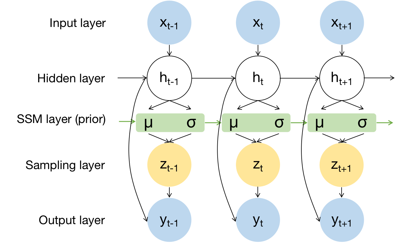
Inspired from Bayer & Osendorfer 2015, Fraccaro et al. 2016 propose the idea of adding stochasticity in a latent state representation on the classical Recurrent Neural Networks (RNN). They stack a state space model (SSM) on deterministic RNNs to achieve a stochastic and sequential generative model (see Figure 1a) and a structured variational inference network (see Figure 1b), which produce the output sequences and provide the model’s posterior distributions, respectively. The loss function includes the negative log-likelihood of the predictions and targets and Kullback-Leibler divergence ($D_{KL}$) (Kullback & Leibler 1951) between the prior and posterior distributions.

This algorithm is expected to be compatible with CARMA models as CARMA can be represented as state space models. The SRNN is applied to the simulated LSST-cadence AGN light curves, and outputs the predicted/interpolated light curves on a daily cadence over 10 years. Figure 2 is an example.

Recently, there has been a discussion in machine learning research: Do better data or better models contribute more to high accuracy? The answer is that for the same model, the accuracy rate increases with the amount of training data, but its ‘marginal utility’ decreases. The capability of models are restricted by the data volume though a better model is able to improve the accuracy to a certain level.

In astronomy, the situation can be more complicated: Data quality is not always sufficient due to weather conditions, satellite interference and other constraints. Accordingly, it is worth discussing whether we should use only ”good” (quality trimmed data) or real data for training, validation, and testing.

While effective data preprocessing methods can greatly improve model results, there are some tricky tasks that developers need to be aware of. For example, how to replace missing values with values that have no significant physical meaning? How to scale, normalize and feed the input data? How to deal with poor-quality data that retains useful information? How to understand the model reflection? Compared with designing model architectures, these issues are more prominent and deserve attention.

In this paper, we discuss the unavoidable problems of real and simulated astronomical data for machine learning applications as well as the limitations of applying SRNN for astronomical time series.

However, the existing difficulties in this project are not uncommon. Researchers are expected to conduct more investigations into the model interpretation and data sets while developing machine learning algorithms and applying them to specific astronomical tasks.

References

- Bayer & Osendorfer (2015) Bayer, J. & Osendorfer, C. 2015, Learning Stochastic Recurrent Networks
- Feigelson et al. (2018) Feigelson, E. D., Babu, G. J., & Caceres, G. A. 2018, Frontiers in Physics, 6, 80
- Fraccaro et al. (2016) Fraccaro, M., Sønderby, S. K., Paquet, U., & Winther, O. 2016, in Proceedings of the 30th International Conference on Neural Information Processing Systems, NIPS’16 (Red Hook, NY, USA: Curran Associates Inc.), 2207–2215
- Kelly et al. (2014) Kelly, B. C., Becker, A. C., Sobolewska, M., Siemiginowska, A., & Uttley, P. 2014, ApJ, 788, 33
- Kozłowski (2017) Kozłowski, S. 2017, A&A, 597, A128
- Kremer et al. (2017) Kremer, J., Stensbo-Smidt, K., Gieseke, F., Pedersen, K. S., & Igel, C. 2017, IEEE Intelligent Systems, 32, 16
- Kullback & Leibler (1951) Kullback, S. & Leibler, R. A. 1951, The Annals of Mathematical Statistics, 22, 79
- LSST Science Collaboration et al. (2009) LSST Science Collaboration, Abell, P. A., Allison, J., et al. 2009, arXiv e-prints, arXiv:0912.0201
- MacLeod et al. (2010) MacLeod, C. L., Ivezic, Z., Kochanek, C. S., et al. 2010, The Astrophysical Journal, 721, 1014–1033
- Maharana et al. (2022) Maharana, K., Mondal, S., & Nemade, B. 2022, Global Transitions Proceedings, 3, 91, international Conference on Intelligent Engineering Approach(ICIEA-2022)
- Moreno et al. (2019) Moreno, J., Vogeley, M. S., Richards, G. T., & Yu, W. 2019, Publications of the Astronomical Society of the Pacific, 131, 063001
- Sánchez-Sáez et al. (2021) Sánchez-Sáez, P., Lira, H., Martí, L., et al. 2021, AJ, 162, 206
- Sheng et al. (2022) Sheng, X., Ross, N., & Nicholl, M. 2022, Monthly Notices of the Royal Astronomical Society, 512, 5580
- Smethurst et al. (2021) Smethurst, R. J., Masters, K. L., Simmons, B. D., et al. 2021, Monthly Notices of the Royal Astronomical Society, 510, 4126
- Tachibana et al. (2020) Tachibana, Y., Graham, M. J., Kawai, N., et al. 2020, The Astrophysical Journal, 903, 54
- Yu & Richards (2022) Yu, W. & Richards, G. T. 2022, EzTao: Easier CARMA Modeling