FedGH: Heterogeneous Federated Learning with Generalized Global HeaderConference: Proceedings of the 31st ACM International Conference on Multimedia; October 29-November 3, 2023; Ottawa, ON, CanadaProceedings of the 31st ACM International Conference on Multimedia (MM ’23), October 29-November 3, 2023, Ottawa, ON, CanadaPrice: 15.00DOI: 10.1145/3581783.3611781ISBN: 979-8-4007-0108-5/23/10CCS: Computing methodologies Distributed artificial intelligenceCCS: Computing methodologies Computer vision tasksCCS: Computing methodologies Computer vision representationsCCS: Computing methodologies Supervised learning by classification

Typical FL. Under FedAvg, a central FL server coordinates $N$ FL clients to collaboratively train a global model. Specifically, in each training round $t$, the server samples a fraction of all the clients, $C$, to join training (i.e., the set of sampled clients joining in the $t$-th round of FL, $|\mathcal{S}^{t}|=C\cdot N=K$). Then, the server broadcasts the global model $\omega$ to the $K$ selected clients. They then train the received global model on their respective local data $D_{k}\sim P_{k}$ ($D_{k}$ obeys the distribution $P_{k}$, i.e., the local data of different clients are non-IID) to obtain $\omega_{k}$ through $\omega_{k}\leftarrow\omega-\eta\nabla\ell\left(\omega;\boldsymbol{x}_{i},y_{i}\right),\left(\boldsymbol{x}_{i},y_{i}\right)\in D_{k}$. The $k$-th client uploads the trained local model $\omega_{k}$ to the server. The server then aggregates them to update the global model as $\omega=\sum_{k=0}^{K-1}\frac{n_{k}}{n}\omega_{k}$. In short, FedAvg aims to minimize the average loss of the global model $\omega$ on all clients’ local data:

where $n_{k}=|D_{k}|$ is the number of samples held by the $k$-th client. $n$ is the number of samples held by all clients. $\mathcal{L}_{k}(\omega)=\ell\left(\omega;D_{k}\right)$ is the loss of the global model $\omega$ with $d$ dimensions on the $k$-th client’s local data $D_{k}$.

The above steps iterate until the global model converges. Since the server averages the received local models, the structures of all clients’ local models must be the same (homogeneous).

Problem Definition for FedGH. We aim to perform FL across clients with heterogeneous models in the same supervised classification tasks. Each client’s local model can be split into two parts: $f\left(\omega_{k}\right)=\mathcal{F}_{k}\left(\varphi_{k}\right)\circ\mathcal{H}_{k}\left(\theta_{k}\right)$, i.e., $\omega_{k}=\left(\varphi_{k},\theta_{k}\right)$, where $\circ$ denotes model splicing. $\mathcal{F}_{k}\left(\varphi_{k};\boldsymbol{x}\right)$: $\mathbb{R}^{d_{\boldsymbol{x}}}\rightarrow\mathbb{R}^{d_{\boldsymbol{\mathcal{R}}}}$ is a feature extractor, which maps local samples from the input feature $\boldsymbol{x}$ to the representation embedding $\boldsymbol{\mathcal{R}}$. $\mathcal{H}_{k}\left(\theta_{k};\mathcal{F}_{k}\left(\varphi_{k};\boldsymbol{x}\right)\right)$: $\mathbb{R}^{d_{\boldsymbol{\mathcal{R}}}}\rightarrow\mathbb{R}^{d_{y}}$ is the prediction header. All clients have the same $d_{\boldsymbol{x}}$, $d_{\boldsymbol{\mathcal{R}}}$, $d_{y}$. We assume that $\mathcal{F}_{k}$ is heterogeneous across different clients (i.e., clients can customize the sizes and structures of local feature extractors to match their system resources and data volume), and all clients share the homogeneous global header $\mathcal{H}(\theta)$ (i.e., all clients carry out the same tasks). That is, $f\left(\omega_{k}\right)=\mathcal{F}_{k}\left(\varphi_{k}\right)\circ\mathcal{H}(\theta)$. So the loss of the $k$-th client’s local model is formulated as $\mathcal{L}_{k}\left(\omega_{k};\boldsymbol{x},y\right)=\mathcal{L}_{\text{sup }}\left(\mathcal{H}\left(\theta;\mathcal{F}_{k}\left(\varphi_{k};\boldsymbol{x}\right)\right),y\right),(\boldsymbol{x},y)\in D_{k}$.

In representation learning (Bengio et al. 2013), representations are the latent feature embedding vectors extracted by feature extractors from input samples. It is hard to infer the original data from the representations without knowing the model parameters (Tan et al. 2022). Therefore, we utilize the representations with the same dimension extracted by different clients’ heterogeneous feature extractors and the corresponding labels (classes) to train a shared global prediction header on the server. It acquires knowledge across all clients and all classes. Clients with homogeneous local models are the special cases of this scenario. We define the training goal of FedGH as minimizing the sum of the losses of all clients’ local heterogeneous models $\{\omega_{0},\ldots,\omega_{N-1}\}$ with dimensions $\{d_{0},\ldots,d_{N-1}\}$:

The workflow of FedGH is displayed in Figure 1. In the $t$-th FL training round, the $k$-th client uses its feature extractor $\varphi_{k}^{t}$ of the local heterogeneous model $\omega_{k}^{t}$ after local training to extract the representations $\boldsymbol{\mathcal{R}}_{k,i}^{t}$ of each local training sample $\left(\boldsymbol{x}_{i},y_{i}\right)$ in $D_{k}$. Then, it calculates the average representation of samples within the same class $s$ as the local averaged representation $\overline{\boldsymbol{\mathcal{R}}}_{k}^{t,s}$ (abbr. LAR) of the corresponding class:

The $k$-th client uploads the LARs $\overline{\boldsymbol{\mathcal{R}}}_{k}^{t,s}$ for each of its local classes and the corresponding class label $s$ to the server. As stated in Tan et al. 2022, the representations are latent feature embedding vectors extracted from the data. Thus, it is hard to infer original data inversely with only extracted representations and without the parameters of the feature extractors. Since each client uploads LARs (i.e., class-wise averaged representations), the risk of privacy leakage is reduced further.

The server inputs all the received LARs $\overline{\boldsymbol{\mathcal{R}}}_{k}^{t,s}$ from $K$ participating clients into the global prediction header $\mathcal{H}$ to produce the prediction. The hard loss (e.g., cross-entropy loss) between the output prediction and the true class label $s$ is used to update the global header parameters $\theta^{t-1}$ via gradient descent:

where $\eta_{\mathcal{\theta}}$ is the learning rate of the global prediction header. To improve the efficiency of training the global prediction header, we allow the server to train the global header once a client’s LARs are received. After the LARs from all participating clients are fed into the global header for training, the global prediction header is updated in the current round. The updated global header acquires all-class knowledge across different clients. Thus, it has a stronger generalization capability than local headers with partial-class knowledge.

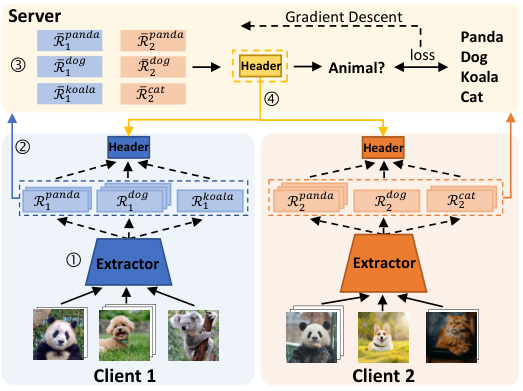
The server broadcasts the updated global header $\theta^{t}$ to the clients selected for the next training round. In the $(t+1)$-th round, the $k$-th client replaces its local prediction header $\theta_{k}^{t}$ with the received global header $\theta^{t}$. In this way, its complete local model becomes:

Intuitively, clients’ local models can converge faster with the generalized global header. Besides, the spliced complete local model obtains the old local knowledge from the personalized heterogeneous feature extractor and the new global knowledge from the shared global header, which enables it to better deal with statistical heterogeneity.

The assembled complete local model $\widetilde{\omega}_{k}^{t+1}$ is trained on local data $D_{k}$ to obtain the updated local model ${\omega}_{k}^{t+1}$:

where $\eta_{\omega}$ is the local model learning rate.

The above steps iterate until all local heterogeneous models converge. The pseudocode for FedGH can be found in Algorithm 1.

Here, we analyze the strength of FedGH in cost reduction and privacy preservation.

Computation Cost. Under FedGH, clients are required to compute the representation for each local training data sample and the averaged representation for samples belonging to the same class. Extracting the representation for one sample is a forward inference of the local model on this sample. Thus, extracting representations only consumes half the computation cost of local training (forward and backwards) in one epoch. Generally, the epochs of local training are set to be larger than 1 in order to avoid frequent communications during FL model training (McMahan et al. 2017). Therefore, extracting representations consumes acceptable computation cost. Besides, since one representation is an $r\times 1$ vector, to calculate the average of representations belonging to each class held by a client, we can first use a “variant” to stack the sum of the representations of each class, and then calculate the average. Therefore, when calculating local average representation (LAR), each client incurs a storage cost and the computational complexity is $\mathcal{O}(n)$, which are negligible compared to the cost of local model training.

On the server side, the computation cost of using LARs to train a shared global header is much lower than training a complete model as the global header is part of a complete model and the number of LARs is far fewer than local data samples. Besides, since the server often has sufficient computation power, training a global header consumes an acceptable portion of its computation resources.

Overall, due to negligible computation cost on both the client and server, FedGH is suitable for both cross-device FL scenarios with resource-constrained mobile edge devices and cross-silo FL scenarios with more powerful participants.

Communication Cost. During the client-to-server uplink communication, clients upload the LAR and the class label for each class to the server. The class label is an integer-type value and the LAR is an $r\times 1$ vector. If each client has $S$ classes, FedGH incurs $(S+S\times r)\times 32$ bits of communication cost, which can be negligible compared to uploading the complete local model in FedAvg.

During server-to-client downlink communication, the server broadcasts the updated global header parameters to clients. This incurs lower communication costs than broadcasting the complete global model to clients in FedAvg. Thus, FedGH is communication-efficient.

Privacy Preservation. During the client-to-server uplink communication, clients upload the LAR and the class label for each class to the server. As stated above, the representation for a sample is an embedding vector mapped by the feature extractor from the original feature space to the embedding space. Thus, it is hard to infer the original data by stealing only representations without knowing the parameters of the feature extractor. Moreover, the uploaded LAR is a mixup of representations within the same class, which further enhances privacy protection.

During the server-to-client downlink communication, the server broadcasts the global prediction header to clients. Since it is part of a complete model, it is also difficult to infer original data by just knowing the global prediction header. Hence, FedGH achieves a high level of privacy preservation. It can be combined with existing privacy protection mechanisms to further enhance FL security.

Datasets and Models. We evaluate FedGH and baselines on two image classification datasets: CIFAR-10 and CIFAR-100 ²² 2 https://www.cs.toronto.edu/%7Ekriz/cifar.html (Krizhevsky et al. 2009), which are manually divided into non-IID datasets following the method in Shamsian et al. 2021. Specifically, for CIFAR-10, we assign only data from 2 out of the 10 classes to each client (non-IID: 2/10). For CIFAR-100, we assign only data from 10 out of the 100 classes to each client (non-IID: 10/100). Then, each client’s local data are further divided into the training set, the evaluation set and the testing set following the ratio of 8:1:1. In this way, the testing set is stored locally by each client which follows the same distribution as the local training set. For the CIFAR-10 and CIFAR-100 datasets, each client trains a CNN model and a ResNet-18 model, respectively. The dimensions of the output layer (i.e., the last fully-connected layer) are $10$ and $100$, and the dimensions of the representation layer (i.e., the second last layer) are set to be $500$.

Baselines. We compare FedGH with the following methods. Standalone, each client trains its local model independently, which serves as a lower bound of model performance. FedAvg (McMahan et al. 2017), a popular FL algorithm that only supports homogeneous local models. The public-data independent model-heterogeneous FL methods include FML (Shen et al. 2020), FedKD (Wu et al. 2022) with mutual learning, LG-FedAvg (Liang et al. 2020) with model mixup, FD (Jeong et al. 2018) with knowledge distillation on logits within the same class, and FedProto (Tan et al. 2022) with knowledge distillation on representations within the same class.

Evaluation Metrics. Accuracy: we measure the accuracy ($\%$) of each client’s local model and report the average test accuracy of all clients’ local models. Communication Overhead (CO): We record the communication overhead ($MB$) incurred upto the point in time when the FL model reaches the target accuracy, which is calculated as (number of rounds required $\times$ the number of clients in each round $\times$ number of floating point data transmitted in the uplink and downlink per round per client $\times$ $32$ bits).

Training Strategy. We tune optimal FL settings for all methods via grid search. The epochs of local training: $E\in\{1,10,30,50,100\}$ and the batch size of local training: $B\in\{32,64,128,256,512\}$. The optimizer of local training is SGD with learning rate $\eta_{\omega}=0.01$. We also tune special hyperparameters for baselines and report the optimal results. Note that FedGH introduces no additional hyperparameters except the global prediction header learning rate $\eta_{\theta}$. We set $\eta_{\theta}=\eta_{\omega}=0.01$ by default. To compare FedGH with the baselines fairly, we set the total number of communication rounds $T\in\{100,500\}$ to guarantee that all algorithms converge.

Training process of FedGH. Client: On the CIFAR-10 (non-IID: 2/10) dataset, each client uses its local heterogeneous feature extractor after local training with learning rate $\eta_{\omega}=0.01$ to extract the representation embedding of each data sample and compute the local averaged representation (LAR) for each class. Then each client uploads LARs and labels of its held 2 classes to the server. Similarly, on CIFAR-100 (non-IID: 10/100) dataset, each client sends 10 classes’ LARs and labels to the server. Server: In the order of client id, the server inputs the LAR of a class from one client into the global header once, then computes the hard loss between the global header output and the label to update the global header via gradient descent with a learning rate $\eta_{\theta}=0.01$. After LARs and labels from all participating clients have been processed, the global header updating in a given round is finished. Furthermore, to accelerate training the global header, we can regard the LARs and the corresponding labels from one client as a batch and allow the server to execute mini-batch gradient descent, which is necessary for the FL scenarios with a large number of clients or classes held by each client.

Model-homogeneous FL can be regarded as a special case of model-heterogeneous FL. Thus, we first evaluate the approaches under the model-homogeneous FL setting before evaluating them under the model-heterogeneous FL setting.

In this section, we evaluate the robustness of the approaches to Non-IIDness and client participation rates, and we also test whether FedGH is sensitive to the only hyperparameter $\eta_{\theta}$ (the learning rate of the global prediction header).