OCELOT: Overlapped Cell on Tissue Dataset for Histopathology
Abstract
Cell detection is a fundamental task in computational pathology that can be used for extracting high-level medical information from whole-slide images. For accurate cell detection, pathologists often zoom out to understand the tissue-level structures and zoom in to classify cells based on their morphology and the surrounding context. However, there is a lack of efforts to reflect such behaviors by pathologists in the cell detection models, mainly due to the lack of datasets containing both cell and tissue annotations with overlapping regions. To overcome this limitation, we propose and publicly release OCELOT, a dataset purposely dedicated to the study of cell-tissue relationships for cell detection in histopathology. OCELOT provides overlapping cell and tissue annotations on images acquired from multiple organs. Within this setting, we also propose multi-task learning approaches that benefit from learning both cell and tissue tasks simultaneously. When compared against a model trained only for the cell detection task, our proposed approaches improve cell detection performance on 3 datasets: proposed OCELOT, public TIGER, and internal CARP datasets. On the OCELOT test set in particular, we show up to improvement in F1-score. We believe the contributions of this paper, including the release of the OCELOT dataset at https://lunit-io.github.io/research/publications/ocelot are a crucial starting point toward the important research direction of incorporating cell-tissue relationships in computation pathology.
1 Introduction

Computational Pathology (CPATH) cpath is a branch of digital pathology that develops methodologies for the analysis of digitized patient specimens, such as Whole-Slide-Images (WSIs). Cell detection in histology images ZHAO2020101786; lal2021nucleisegnet; qu2020weakly is one of the most important tasks in CPATH. It allows the quantification and analysis of different cell types, which can lead to better prognosis evaluation SUN2021103492; park2022artificial and patient treatment planning while maintaining medical interpretability diao2021human. Since it has the potential to impact human lives, high-performance cell detection models are essential in real-world applications and need to be investigated.
To better locate and classify cells, detailed morphological characteristics such as color and shape are crucial. Consequently, cell detection datasets are typically collected at high magnification but small Field-of-View (FoV). However, this can make the cell detection model overly rely on appearance details, without understanding the broader context awmfovnet. This context can help cell detection by providing information about how cells are arranged and grouped together to form high-level tissue structures. In practice, expert annotators (pathologists) first zoom out to understand these broad tissue structures. Next, they zoom in to better classify individual cells while taking into account the context information, as depicted in Fig. 1.
The behavior of pathologists can be transferred to deep learning, for instance, through a multi-task strategy combining cell detection tasks at high magnification and tissue segmentation at low magnification. This type of approach would allow the model to share knowledge across different tasks and FoVs. However, to train such an approach, a combined dataset with cell-tissue overlapping regions is required; unfortunately, most existing datasets only target a single task, either cell detection MoNuSeg; GRAHAM2019101563 or tissue segmentation PANDA; digestpath.
In this paper, we introduce a new research direction: studying cell-tissue relationships for cell detection. First, we publish the OCELOT dataset, which contains cell and tissue annotations in small and large FoV patches, respectively, with overlapping regions. Additionally, the data is collected from WSIs of multiple organs. This can provide the necessary data for researchers to study cell-tissue relationships and their effect on cell detection. Second, we introduce simple multi-task learning approaches for cell detection that can benefit from cell-tissue relationships and demonstrate their advantages over 3 different datasets. These approaches consistently show better cell detection performance compared to the cell-only baseline, i.e., a model trained only with small FoV patches with the corresponding cell annotations. We hope that our proposed OCELOT dataset and methods will encourage the CPATH community to learn how to reflect cell-tissue relationships better to improve cell detection.
Our contributions are 3-fold and summarized as follows,
- •
The first work that exploits cell-tissue relationships for better cell detection, to the best of our knowledge.
- •
We release OCELOT, a dataset with overlapping cell and tissue annotations based on Hematoxylin and Eosin (H&E) stained WSIs of multiple organs.
- •
We introduce several approaches that boost cell detection performance via multi-task learning, and empirically confirm that these methods generalize well across different datasets and histological stainings.
2 Related Work
2.1 Datasets for Cell detection and Tissue segmentation Tasks
In recent years, numerous datasets have been released for tackling cell detection. Some of those works only target a single organ TNBC; GRAHAM2019101563, while others consider multiple ones CPM17; MoNuSeg; MoNuSAC; PanNuke; NuCLS. The availability of these datasets enables the CPATH community to push forward the development and improvement of cell detection models GRAHAM2019101563; ZHAO2020101786; liu2019nuclei; lal2021nucleisegnet; li2019dual; qu2020weakly. In addition, tissue segmentation datasets have also been proposed for prostate NIR2018167; 8853320; PANDA, colorectal tissue_ds_1, brain miccai2014, and multiple organs ADP. Some examples of tissue segmentation works can be found in tissue_ds_2; chan2019histosegnet; zhu2021multi; chen2016dcan; qian2022transformer; li2016gland. The dataset in digestpath is composed of a cell detection subset and a tissue segmentation subset. However, the subsets are annotated independently and from different patient groups, and, therefore, there are no overlaps between the cell and tissue data. Because of the lack of overlapping data in the aforementioned datasets, it is difficult to build an end-to-end framework to learn cell-tissue relationships by jointly training on the cell and tissue tasks.
The recently released TIGER dataset tiger contains both cell and tissue annotations to study tumor-infiltrating lymphocytes SALGADO2015259 in H&E breast cancer WSIs. All the cell-annotated areas exist inside the tissue-annotated area, however, this work does not propose nor initiate any effort toward the integration of both cell and tissue tasks.
| Dataset | Tissue Area | # Cell | Organs | |
|---|---|---|---|---|
| OCELOT | 4.267 | 114.7K | multiple | |
| TIGER | 2.536 | 50.8K | breast |
To further promote the development of methods that leverage the cell-tissue relationship for the task of cell detection, we propose OCELOT, which is designed to capture the hierarchical relationship between cells and tissues, especially in the tumor environment. OCELOT contains roughly two times more cell and tissue annotations than TIGER (see Tab. 1). Additionally, the data was collected from multiple organs to enable the investigation of the generalizability of cell-tissue relationships over various cancer types. In the end, we utilized both OCELOT and TIGER to reveal the power of cell-tissue relationship for cell detection in Sec. 6.
2.2 Leveraging Large Field of View
Some studies KAMNITSAS201761; awmfovnet; VANRIJTHOVEN2021101890; SCHMITZ2021101996; HO2021101866; 10.1007/978-3-030-59722-1_37 extract a large FoV region as an additional input to improve detection/segmentation performance on smaller FoV regions. KAMNITSAS201761 proposes a dual pathway 3D CNN for brain lesion segmentation, where each pathway receives both small and large center-shared FoV regions as input. Similar studies are also conducted in the CPATH domain for tissue segmentation awmfovnet; VANRIJTHOVEN2021101890; SCHMITZ2021101996; HO2021101866 and cell detection 10.1007/978-3-030-59722-1_37. To fuse different FoV patches, awmfovnet introduces a weighting mechanism and VANRIJTHOVEN2021101890 proposes a multi-scale merging block composed of convolution and concatenation. Nevertheless, no inter-task relationship is considered in the previously mentioned methods. In contrast, our models take advantage of the large contextual information while learning the cell-tissue relationship via multi-task objectives at different FoVs.
2.3 Leveraging Cell-Tissue Relationships
To our understanding, there is no study that considers cell-tissue relationships for cell detection or tissue segmentation tasks. On the other hand, a few efforts have attempted to link tissue and cell for image classification using graph-based methods cgcnet; wsptcgcn; hactnet. Such studies represent the tissue structure as a graph of detected cells, based on the medical knowledge that cells form tissues. hactnet explicitly considers the cell-tissue relationship for the task of breast cancer subtyping, by an interaction between tissue-level and cell-level graphs with a cell-to-tissue hierarchy. However, these methods treat the cell/tissue graph generation as a pre-processing step, by using the inference output of independently pre-trained cell detection and tissue segmentation models. In contrast, we directly target the improvement of cell detection by utilizing the cell-tissue relationship.
3 OCELOT
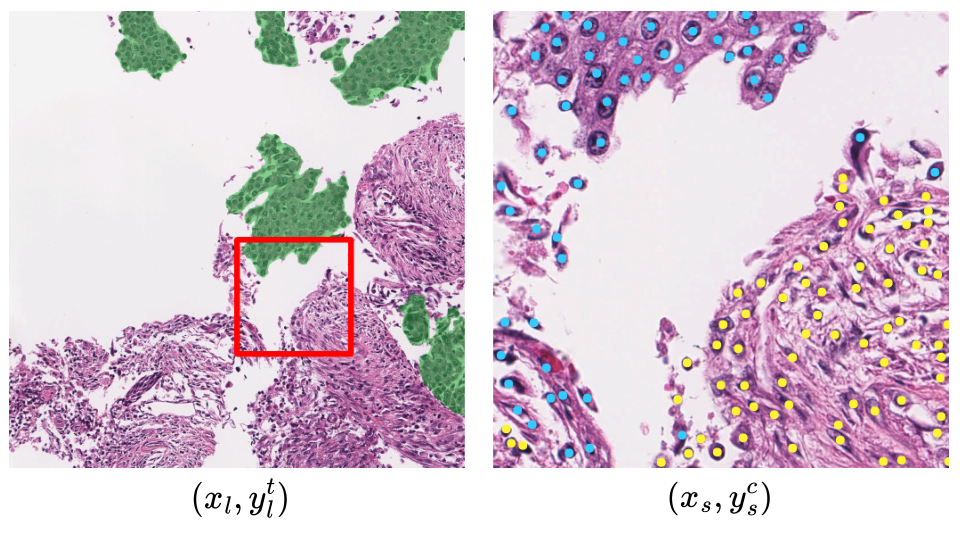
In this section, we introduce OCELOT, a histopathology dataset specifically built to enable the development of methods that leverage cell and tissue relationships. Each sample of the OCELOT dataset is composed of six components,
| (1) |
where are the small and large FoV patches extracted from the WSI, refer to the corresponding cell and tissue annotations, respectively, and are the relative coordinates of the center of within . We drop the sample index for simplicity. Fig. 2 shows the visualization of a sample in OCELOT. More details about the dataset including data collection and statistics can be found in the following sub-sections. The dataset is publicly available at https://lunit-io.github.io/research/publications/ocelot/.
3.1 Data Collection
We collect 306 TCGA HUTTER2018283 WSIs from a total of 6 different organs: kidney, head-and-neck, prostate, stomach, endometrium, and bladder. From each of the WSIs, we select 1 to 3 large Regions of Interest (ROIs) for the tissue segmentation task. Finally, for the cell detection task, we randomly choose a smaller ROI that is fully contained within the larger tissue ROI. As a result, OCELOT includes 673 paired patches from 6 organs. The numbers of WSIs and pairs of patches per organ are detailed in Tab. 2.
Some natural image datasets, such as ImageNet deng2009imagenet or Pascal VOC everingham2010pascal, include thousands of annotated images. However, annotating histopathology images is more challenging and expensive due to the scarcity of expert pathologists c3det. Furthermore, acquiring dense annotations for cell detection and tissue segmentation is especially time-demanding compared to higher-level tasks such as image classification. Nonetheless, in Tab. 1, we observe that OCELOT is roughly double the size of the recent TIGER dataset with respect to the annotated tissue area and the number of annotated cells.
Patch configuration.
Cell detection tasks benefit from fine-grained spatial information to better capture detailed cell properties (e.g. border, shape, color, and opacity). In contrast, tissue segmentation requires a larger context to enable a better understanding of the overall structural information. Therefore, we define the FoV sizes of (cell detection) and (tissue segmentation) as 1024 1024 and 4096 4096 pixels, respectively, at a resolution of 0.2 Microns-per-Pixel (MPP). Finally, the large FoV patches and tissue annotations (, ) are down-sampled by a factor of 4, resulting in a size of 1024 1024 pixels.
Annotation.
All cell-tissue pairs of patches are annotated by board-certified pathologists. Cells are labeled as points, with associated 2D coordinates and class labels. We denote the annotations in a given cell-level patch, , as , and consider two classes: Tumor Cell (TC) and Background Cell (BC)11 1 BC includes any of the following cell categories: lymphocyte, macrophage, fibroblast, endothelial, or other remaining cell types.. TC and BC class ratios are 35.01% and 64.99%, respectively. Regarding the tissue patches, , pathologists annotate the pixel-wise segmentation maps with either Cancer Area (CA) or Background (BG) labels. A minority of pixels where the tissue class was uncertain were labeled as Unknown (UNK). BG, CA, and UNK class ratios are 55.77%, 40.17%, and 4.06%, respectively. The amount of annotated cells and tissue pixels, per data split, can be found in the supplementary material. The detection of TC and BC has clinical relevance. For example, tumor purity azimi2017breast, computed as the tumor/non-tumor cell ratio in a WSI, has a correlation with cancer prognosis mao2018low; zhang2017tumor; gong2020tumor.
Dataset splits.
The dataset is divided into three subsets: training, validation, and test, following a :: ratio. To prevent information leaking among the data subsets, we randomly split the dataset per WSI, so that different patches from the same WSI are not included in multiple subsets. We maintain consistent cancer-type ratios in each subset.
| Organs | # Slides | # Patch Pairs | ||||
|---|---|---|---|---|---|---|
| Train | Val | Test | Train | Val | Test | |
| Kidney | 48 | 15 | 18 | 125 | 41 | 41 |
| Head-neck | 13 | 5 | 6 | 27 | 9 | 10 |
| Prostate | 26 | 12 | 10 | 50 | 17 | 16 |
| Stomach | 15 | 6 | 5 | 36 | 12 | 12 |
| Endometrium | 38 | 13 | 13 | 86 | 29 | 25 |
| Bladder | 35 | 14 | 14 | 82 | 29 | 26 |
| Total | 175 | 65 | 66 | 406 | 137 | 130 |
4 Empirical Analysis
The motivation for considering the cell-tissue relationships for the development of cell detection models stem from the biological and hierarchical arrangement of cells and tissues. These insights are further corroborated by two main empirical observations described in the following Sec. 4.1 and Sec. 4.2.
4.1 Interrelation between cell and tissue classes
| Cell | Tissue | Cell | Tissue | |||
| CA | non-CA | ST | non-ST | |||
| TC | 67.7K | 5.4K | LC | 45.4K | 5.4K | |
| BC | 6.4K | 35.2K | ||||
| (a) OCELOT | (b) TIGER | |||||
| CA | non-CA | ST | non-ST | |
| 40.17% | 59.83% | 30.79% | 69.21% | |
| (a) OCELOT | (b) TIGER | |||
We empirically observe the interrelation between specific cell and tissue classes by counting the amount of each annotated cell type within each tissue region, as observed in Tab. 3. Indeed, we verify that in OCELOT, around 93% of TC are located within CA and 85% of BC are found outside of the CA tissue. Note that CA is not the majority tissue class (Tab. 4), therefore, we conclude that there is, in fact, a relationship between the cell and tissue classes. We observe a similar phenomenon in the TIGER dataset when considering the LC and ST classes (Tab. 3 and Tab. 4).
In practice, pathologists classify cells by taking into account such interrelationships, since it is difficult to classify isolated cells, without considering the larger context of the tissues. As depicted in Fig. 1, pathologists first need to visualize the structure of the tissues at a larger FoV. Then, they zoom in and consider the previously observed context along with the fine-grained details of each individual cell and nearby neighborhood, thus considering the cell-tissue dependencies. Inspired by the behavior of pathologists, we expect a cell detection model to also benefit from understanding the tissue structure from a broader viewpoint.
4.2 Tissue-label Leaking Model
In the previous section, we observe a strong relationship between certain cell and tissue classes. To further validate the hypothesis that a cell detection model can leverage information from the tissue structure, we design an exploratory experiment where the tissue annotation is provided as an extra input to a cell detection model. To this end, we first crop the corresponding cell patch region from the tissue annotation , and upsample it to match the size of the cell patch, ; the cropped tissue annotation is denoted as . Finally, we concatenate and at the channels dimension and use this data to train a cell detection model. We denote this model as a Tissue-label leaking model and illustrate it in Fig. 3. Note that this model is not appropriate for real-world scenarios as the tissue labels are unknown at inference time, and is explored for the purpose of empirical analysis.
When we compare the performance of the tissue-label leaking model with the standard cell detection model on the OCELOT dataset, we observe a significant improvement in terms of mean F1-score22 2 True positive (TP), false positive (FP), and false negative (FN) counts are determined following SwiderskaChadaj2019LearningTD. If a detected cell is within a valid distance () from an annotated cell and the cell class matches, it is counted as a TP, otherwise an FP. If an annotated cell is not detected, it is counted as an FN. Then, the mean F1 score across classes is computed. performance of +7.69 and +9.76 in the validation and test sets, respectively. Detailed results can be found in Tab. 5. Taking these results into consideration, we conclude that there is significant room to improve the cell detection model, which can be achieved by combining the tasks of cell detection and tissue segmentation.

5 Method
In this section, we propose to utilize cell-tissue relationships through multi-task learning. First, we propose a set of approaches inspired by the tissue-label leaking model described in Sec. 4.2. These models replace the annotated tissue labels with predictions from an auxiliary tissue segmentation branch. Second, we design a bi-directional information-sharing approach that shares features in both tissue-to-cell and cell-to-tissue directions. The proposed approaches are described in Sec. 5.2 and Sec. 5.3
5.1 Preliminary
To deal with cell-tissue sample pairs, i.e., and , we build a dual-branch architecture containing separate networks for the cell and tissue tasks. Similarly to SwiderskaChadaj2019LearningTD, we define cell detection as a segmentation task. Specifically, the cell labels are provided as a segmentation map by drawing a fixed-radius circle centered on each cell point annotation and filled with the corresponding class label. At inference time, we find local peaks within the predicted cell probability maps and output them as point predictions. More details are provided in the supplementary material. Treating cell detection as a segmentation task enables us to use the same architecture for both cell and tissue branches, which largely simplifies the training and tuning of the model and reduces the range of possible decisions, such as neural network architecture, or hyper-parameters. We use DeepLabV3+ deeplabv3plus2018 as a base architecture for both branches and single-task models.
5.2 Tissue-prediction Injection Models
These models are a simple and practical extension of the tissue-label leaking model, where we inject the predicted tissue probabilities into the cell detection branch instead of leaking the tissue labels. We consider only one injection point in the cell detection branch, but explore four possible alternatives: (a) at the input (Pred-to-input), (b) after the encoder (Pred-to-inter-1), (c) after the ASPP module (Pred-to-inter-2), and (d) after the decoder (Pred-to-output). Fig. 4 depicts this family of models, denominated as Tissue-prediction injection. Since the tissue and cell patches represent different regions, we need to align the content between the tissue and cell feature maps before concatenation. Therefore, we crop the cell corresponding region from the tissue predictions, upsample them, and, finally, concatenate them in the channel dimensions of the feature maps of the cell branch, as illustrated in 5(a).

5.3 Cell-Tissue Feature Sharing Model
Tissue-prediction injection models share the tissue prediction in a single location and direction, i.e., tissue-to-cell. To enable a more diverse and flexible cell-tissue information flow, we also explore bi-directional feature map sharing from cell-to-tissue (Fig. 5, left) and tissue-to-cell (Fig. 5, right). Considering these two operations, we conduct an architecture search procedure to find the optimal feature map sharing configuration between both branches. To limit the search space, we constrain it to only 3 positions in the architecture: after the encoder, after the ASPP module, or after the decoder. Furthermore, we also exclusively allow the branches to inject feature maps at the same depth or position. Finally, we consider only the best-performing model among the candidates, which is presented in Fig. 6. We name this model as cell-tissue feature sharing.


6 Experiments and Results
| Method | OCELOT | TIGER | CARP | |||
|---|---|---|---|---|---|---|
| Val | Test | Val | Test | Val | Test | |
| Cell-only | 68.871.76 | 64.441.82 | 63.891.39 | 53.821.23 | 78.480.69 | 70.961.47 |
| Pred-to-input | 73.360.59 | 69.653.93 | 66.002.00 | 53.291.30 | 79.460.79 | 72.980.82 |
| Pred-to-inter-1 | 72.740.50 | 70.542.20 | 66.191.02 | 55.871.78 | 79.740.80 | 73.050.69 |
| Pred-to-inter-2 | 72.681.58 | 71.230.96 | 65.431.14 | 54.752.25 | 79.870.78 | 73.141.53 |
| Pred-to-output | 66.855.62 | 65.053.72 | 63.020.16 | 53.320.42 | 78.920.60 | 72.610.95 |
| Feature-sharing | 72.300.73 | 68.912.52 | 65.641.07 | 55.102.18 | 79.380.74 | 73.000.33 |
| Tissue-label leaking | 76.560.80 | 74.200.91 | 69.710.61 | 61.661.16 | 80.131.04 | 72.970.49 |
| Method | population | kidney | endometrium | bladder | prostate | stomach | head-neck |
|---|---|---|---|---|---|---|---|
| (130) | (41) | (25) | (26) | (16) | (12) | (10) | |
| Cell-only | 64.441.82 | 64.123.41 | 66.883.71 | 59.425.61 | 65.461.64 | 66.198.93 | 59.245.04 |
| Pred-to-input | 69.653.93 | 63.373.27 | 73.316.35 | 63.614.55 | 68.368.61 | 69.347.15 | 75.280.82 |
| Pred-to-inter-1 | 70.542.20 | 66.627.30 | 73.054.14 | 64.353.59 | 70.202.56 | 71.555.21 | 74.501.52 |
| Pred-to-inter-2 | 71.230.96 | 68.945.65 | 75.152.70 | 64.942.34 | 68.358.83 | 70.290.81 | 73.741.72 |
| Pred-to-output | 65.053.72 | 63.384.48 | 68.214.11 | 59.813.96 | 64.188.41 | 67.516.39 | 60.886.77 |
| Feature-sharing | 68.912.52 | 64.975.33 | 71.285.30 | 63.215.31 | 66.259.52 | 69.792.25 | 73.884.39 |
| Tissue-label leaking | 74.200.91 | 75.751.97 | 72.711.12 | 71.180.93 | 74.561.25 | 75.241.71 | 75.780.46 |
We validate the hypothesis that incorporating cell-tissue relationships within a cell detection model is beneficial by evaluating the proposed models on OCELOT and 2 other datasets. First, we describe the additional datasets and implementation details. Then, we show how the proposed multi-task learning methods can improve the performance of a cell detection task. Lastly, we conduct an ablation study to investigate how important using large FoV patches and corresponding tissue segmentation labels are in enhancing cell-tissue relationships.
6.1 Other Datasets
TIGER.
As mentioned in Sec. 2.1, TIGER is a public dataset, based on H&E stained images, which includes both cell and tissue annotations in overlapping patches. However, the patch sizes and amount of overlap between cell and tissue annotations highly vary among samples. Therefore, a pre-processing step is necessary to generate paired cell-tissue patches with consistent FoVs. After pre-processing, we obtain 9,888 paired patches of size 512512 and 128128 pixels for the tissue segmentation and cell detection tasks, respectively, with an MPP of approximately 0.5 . Most samples in TIGER include small regions with annotated cells, making it necessary to extract smaller patches. This explains why the absolute number of patches is larger than in OCELOT or CARP, although the actual amount of annotated cells and tissue area are smaller than the latter datasets, as shown in Tab. 1. In TIGER, one cell class (lymphocyte cells) and seven tissue classes are annotated. More details about the pre-processing and this dataset are provided in the supplementary material.
CARP.
This is an internal lung cancer dataset of PD-L1 IHC-stained WSIs, containing 6,480 paired patches extracted from 1,012 WSIs. The patch sizes, resolution, annotation protocol, and general configuration are similar to OCELOT, as described in Sec. 3.1. Two cell classes are annotated: PD-L1 positive tumor cells (TC+), and PD-L1 negative tumor cells (TC-). The tissue classes are the same as in OCELOT (BG, CA, and UNK). CARP is a real-world and large-scale dataset, with 809.1K annotated cells and 4.1080 tissue area, which is approximately 10 and 20 times more than OCELOT and TIGER, respectively. Moreover, the stain type is different from OCELOT and TIGER, allowing us to validate the effectiveness of the cell-tissue relationships across different staining methods.
6.2 Implementation details
As previously mentioned in Sec. 5.1, both cell and tissue branches are based on DeepLabV3+ deeplabv3plus2018, with a ResNet-34 He2015 encoder. The models are trained for 300, 150, and 100 epochs in OCELOT, TIGER, and CARP datasets, respectively. We use the Adam optimizer KingmaB14, and, for each experiment, we tune the learning rate within a range. The model at the epoch with the best validation set performance is chosen and used for evaluation on the test set. All experiments are repeated 5 times, and we report the mean and 95% confidence interval of the performance metrics. For more implementation details, please refer to the supplementary material.
6.3 Main Results
The cell detection results obtained by the Cell-only baseline, the proposed approaches, and the Tissue-label leaking model are shown in Tab. 5. The Cell-only baseline is a simple cell detection model that only receives the small FoV patches as input. In other words, it only considers the cell branch in Fig. 4 and neither tissue annotations nor large FoV patches are leveraged. The Tissue-label leaking model, described in Sec. 5.2, receives the tissue annotations as input and serves as an exploratory experiment to obtain insight regarding how much the cell detection task can benefit from leveraging tissue annotation.
From Tab. 5, we observe that all the cell-tissue multi-task learning-based approaches, except for the Pred-to-output model, outperform the Cell-only baseline across all datasets. These improvements imply that cell detection on small FoV patches benefits from learning cell-tissue interrelationships from both large FoVs and tissue annotations. We hypothesize that the reason for the low performance of the Pred-to-output model is that the injection of tissue prediction to the cell branch happens too late. Therefore, there is a lack of network capacity for fusing cell and tissue information.
Furthermore, in Tab. 6, we report mean F1 scores per organ in the OCELOT test set. Except for the Pred-to-output, all approaches show improvement compared to Cell-only baseline in most organs. Especially, our best-performing model, Pred-to-inter-2, demonstrates superior performance over Cell-only in all 6 organs with a significant margin. Such a result shows that considering cell-tissue relationships can generally help the cell detection task across various organs.
| Further utilize | Pred-to-inter-2 | Feature-sharing | |||
|---|---|---|---|---|---|
| Tissue label | Large FoV | Val | Test | Val | Test |
| - | - | 68.871.76 | 64.451.82 | 68.871.76 | 64.451.82 |
| ✓ | - | 70.211.49 | 64.991.77 | 70.361.34 | 66.582.02 |
| - | ✓ | 68.780.94 | 65.563.66 | 69.611.59 | 66.221.53 |
| ✓ | ✓ | 72.681.58 | 71.230.96 | 72.300.73 | 68.912.52 |

6.4 Dataset Ablation Study
Two data components in OCELOT contribute to better leveraging cell-tissue relationships for the task of cell detection: (1) the large FoV patches , and (2) the corresponding tissue annotations that allows us to have a tissue segmentation objective and a multi-task learning setting. To verify the effectiveness of each data component, we conduct an ablation study where each component is evaluated separately while keeping the model architecture fixed. First, if only the tissue segmentation label is provided without a large FoV patch, the tissue branch takes as an input and it is trained with both the tissue and the cell detection objectives. Second, if the large FoV patch is given without the corresponding tissue label, the tissue branch takes as an input and the model is only trained with the cell detection objective.
The results of the ablation study are shown in Tab. 7. We observe that each of the individual components on their own lead to improved performance. Hence, we can conclude that a large FoV patch and tissue segmentation label can contribute to better cell detection by providing a broader context and encoding the cell-tissue relationship, respectively. Moreover, when utilized simultaneously, we observe that both components work synergetically, leading to an even better performance improvement. We also found that the tissue branch generates better tissue predictions when trained with a large FoV. Thus, providing accurate tissue information to the cell branch is important for boosting performance. Please, refer to the supplementary material for a detailed tissue performance comparison. Finally, this study shows evidence that the patch configuration defined in OCELOT is suitable for cell-tissue co-training, with a smaller FoV for cell detection and a larger FoV for tissue segmentation .
6.5 Qualitative Analysis
In this section, we visualize the cell predictions of the Cell-only and Pred-to-inter-2 models. We select the Pred-to-inter-2 model, as it is the overall best-performing model in our experiments. In general, when compared to other background cells, tumor cells have the following characteristics: large size and irregular shape. However, cancer is heterogeneous and this is not always the case. Indeed, in Fig. 7, most of the cells are small and have a regular round shape. Based on these appearances, and without a larger context, those cells can be easily misclassified as background cells, which is the case of the Cell-only model. On the other hand, Pred-to-inter-2 shows a more accurate prediction by correctly understanding the cancer area in large FoV regions. This implies that Pred-to-inter-2 indeed considers both the morphology of cells and the tissue context, while Cell-only relies on the cells’ morphology alone.
7 Conclusion
In histopathology, there is a hierarchical organization and interrelationship between cells and tissues. Hence, we hypothesize that it can be leveraged to improve the performance of cell detection tasks. Throughout this paper, we have shown evidence that such cell-tissue relationships exist across multiple setups. Indeed, we observe improvements when utilizing large FoVs with corresponding tissue annotations together with cell annotations in a multi-task learning approach, using simple neural architecture designs. Although the cell detection task clearly benefits from the multi-task learning framework, the improvement on the tissue segmentation task was not yet investigated, and we leave this topic as a future direction. We hope this work, especially the OCELOT dataset, initiates new and promising research directions in CPATH to further study the cell-tissue relationships and improve cell detection and tissue segmentation.
References
- (1) MICCAI 2014 Grand Challenges. https://wiki.cancerimagingarchive.net/display/Public/MICCAI+2014+Grand+Challenges, 2014. [Online; accessed Nov-2022].
- (2) TIGER: Grand Challenge. https://tiger.grand-challenge.org, 2022. [Online; accessed Nov-2022].
- (3) Esther Abels, Liron Pantanowitz, Famke Aeffner, Mark D Zarella, Jeroen van der Laak, Marilyn M Bui, Venkata NP Vemuri, Anil V Parwani, Jeff Gibbs, Emmanuel Agosto-Arroyo, et al. Computational pathology definitions, best practices, and recommendations for regulatory guidance: a white paper from the digital pathology association. The Journal of Pathology, 249(3):286–294, 2019.
- (4) Mohamed Amgad, Lamees A Atteya, Hagar Hussein, Kareem Hosny Mohammed, Ehab Hafiz, Maha AT Elsebaie, Ahmed M Alhusseiny, Mohamed Atef AlMoslemany, Abdelmagid M Elmatboly, Philip A Pappalardo, et al. Nucls: A scalable crowdsourcing approach and dataset for nucleus classification and segmentation in breast cancer. GigaScience, 11, 2022.
- (5) Vahid Azimi, Young Hwan Chang, Guillaume Thibault, Jaclyn Smith, Takahiro Tsujikawa, Benjamin Kukull, Bradden Jensen, Christopher Corless, Adam Margolin, and Joe W Gray. Breast cancer histopathology image analysis pipeline for tumor purity estimation. In 2017 IEEE 14th International Symposium on Biomedical Imaging (ISBI 2017), pages 1137–1140. IEEE, 2017.
- (6) Tian Bai, Jiayu Xu, and Fuyong Xing. Multi-field of view aggregation and context encoding for single-stage nucleus recognition. In MICCAI, pages 382–392. Springer, 2020.
- (7) Wouter Bulten, Kimmo Kartasalo, Po-Hsuan Cameron Chen, Peter Ström, Hans Pinckaers, Kunal Nagpal, Yuannan Cai, David F Steiner, Hester van Boven, Robert Vink, et al. Artificial intelligence for diagnosis and gleason grading of prostate cancer: the panda challenge. Nature Medicine, 28(1):154–163, 2022.
- (8) Lyndon Chan, Mahdi S Hosseini, Corwyn Rowsell, Konstantinos N Plataniotis, and Savvas Damaskinos. Histosegnet: Semantic segmentation of histological tissue type in whole slide images. In ICCV, pages 10662–10671, 2019.
- (9) Hao Chen, Xiaojuan Qi, Lequan Yu, and Pheng-Ann Heng. Dcan: deep contour-aware networks for accurate gland segmentation. In CVPR, pages 2487–2496, 2016.
- (10) Liang-Chieh Chen, Yukun Zhu, George Papandreou, Florian Schroff, and Hartwig Adam. Encoder-decoder with atrous separable convolution for semantic image segmentation. In ECCV, pages 801–818, 2018.
- (11) Qian Da, Xiaodi Huang, Zhongyu Li, Yanfei Zuo, Chenbin Zhang, Jingxin Liu, Wen Chen, Jiahui Li, Dou Xu, Zhiqiang Hu, et al. Digestpath: a benchmark dataset with challenge review for the pathological detection and segmentation of digestive-system. Medical Image Analysis, page 102485, 2022.
- (12) Jia Deng, Wei Dong, Richard Socher, Li-Jia Li, Kai Li, and Li Fei-Fei. Imagenet: A large-scale hierarchical image database. In CVPR, pages 248–255. Ieee, 2009.
- (13) James A Diao, Jason K Wang, Wan Fung Chui, Victoria Mountain, Sai Chowdary Gullapally, Ramprakash Srinivasan, Richard N Mitchell, Benjamin Glass, Sara Hoffman, Sudha K Rao, et al. Human-interpretable image features derived from densely mapped cancer pathology slides predict diverse molecular phenotypes. Nature communications, 12(1):1–15, 2021.
- (14) Mark Everingham, Luc Van Gool, Christopher KI Williams, John Winn, and Andrew Zisserman. The pascal visual object classes (voc) challenge. IJCV, 88(2):303–338, 2010.
- (15) Jevgenij Gamper, Navid Alemi Koohbanani, Ksenija Benes, Simon Graham, Mostafa Jahanifar, Syed Ali Khurram, Ayesha Azam, Katherine Hewitt, and Nasir Rajpoot. Pannuke dataset extension, insights and baselines. arXiv preprint arXiv:2003.10778, 2020.
- (16) Zhe Gong, Jieyun Zhang, and Weijian Guo. Tumor purity as a prognosis and immunotherapy relevant feature in gastric cancer. Cancer Medicine, 9(23):9052–9063, 2020.
- (17) Simon Graham, Quoc Dang Vu, Shan E Ahmed Raza, Ayesha Azam, Yee Wah Tsang, Jin Tae Kwak, and Nasir Rajpoot. Hover-net: Simultaneous segmentation and classification of nuclei in multi-tissue histology images. Medical Image Analysis, 58:101563, 2019.
- (18) Kaiming He, Xiangyu Zhang, Shaoqing Ren, and Jian Sun. Deep residual learning for image recognition. pages 770–778, 2016.
- (19) David Joon Ho, Dig VK Yarlagadda, Timothy M D’Alfonso, Matthew G Hanna, Anne Grabenstetter, Peter Ntiamoah, Edi Brogi, Lee K Tan, and Thomas J Fuchs. Deep multi-magnification networks for multi-class breast cancer image segmentation. Computerized Medical Imaging and Graphics, 88:101866, 2021.
- (20) Mahdi S Hosseini, Lyndon Chan, Gabriel Tse, Michael Tang, Jun Deng, Sajad Norouzi, Corwyn Rowsell, Konstantinos N Plataniotis, and Savvas Damaskinos. Atlas of digital pathology: A generalized hierarchical histological tissue type-annotated database for deep learning. In CVPR, pages 11747–11756, 2019.
- (21) Carolyn Hutter and Jean Claude Zenklusen. The cancer genome atlas: creating lasting value beyond its data. Cell, 173(2):283–285, 2018.
- (22) Konstantinos Kamnitsas, Christian Ledig, Virginia FJ Newcombe, Joanna P Simpson, Andrew D Kane, David K Menon, Daniel Rueckert, and Ben Glocker. Efficient multi-scale 3d cnn with fully connected crf for accurate brain lesion segmentation. Medical Image Analysis, 36:61–78, 2017.
- (23) Davood Karimi, Guy Nir, Ladan Fazli, Peter C Black, Larry Goldenberg, and Septimiu E Salcudean. Deep learning-based gleason grading of prostate cancer from histopathology images—role of multiscale decision aggregation and data augmentation. IEEE journal of Biomedical and Health Informatics, 24(5):1413–1426, 2019.
- (24) Diederik P Kingma and Jimmy Ba. Adam: A method for stochastic optimization. In ICLR, 2015.
- (25) Neeraj Kumar, Ruchika Verma, Deepak Anand, Yanning Zhou, Omer Fahri Onder, Efstratios Tsougenis, Hao Chen, Pheng-Ann Heng, Jiahui Li, Zhiqiang Hu, et al. A multi-organ nucleus segmentation challenge. IEEE transactions on Medical Imaging, 39(5):1380–1391, 2019.
- (26) Shyam Lal, Devikalyan Das, Kumar Alabhya, Anirudh Kanfade, Aman Kumar, and Jyoti Kini. Nucleisegnet: robust deep learning architecture for the nuclei segmentation of liver cancer histopathology images. Computers in Biology and Medicine, 128:104075, 2021.
- (27) Chunggi Lee, Seonwook Park, Heon Song, Jeongun Ryu, Sanghoon Kim, Haejoon Kim, Sérgio Pereira, and Donggeun Yoo. Interactive multi-class tiny-object detection. In CVPR, pages 14136–14145, 2022.
- (28) Wenqi Li, Siyamalan Manivannan, Shazia Akbar, Jianguo Zhang, Emanuele Trucco, and Stephen J McKenna. Gland segmentation in colon histology images using hand-crafted features and convolutional neural networks. In 2016 IEEE 13th international symposium on biomedical imaging (ISBI), pages 1405–1408. IEEE, 2016.
- (29) Xieli Li, Yuanyuan Wang, Qisheng Tang, Zhen Fan, and Jinhua Yu. Dual u-net for the segmentation of overlapping glioma nuclei. Ieee Access, 7:84040–84052, 2019.
- (30) Dongnan Liu, Donghao Zhang, Yang Song, Chaoyi Zhang, Fan Zhang, Lauren O’Donnell, and Weidong Cai. Nuclei segmentation via a deep panoptic model with semantic feature fusion. In IJCAI, pages 861–868, 2019.
- (31) Yihao Mao, Qingyang Feng, Peng Zheng, Liangliang Yang, Tianyu Liu, Yuqiu Xu, Dexiang Zhu, Wenju Chang, Meiling Ji, Li Ren, et al. Low tumor purity is associated with poor prognosis, heavy mutation burden, and intense immune phenotype in colon cancer. Cancer Management and Research, 10:3569, 2018.
- (32) Peter Naylor, Marick Laé, Fabien Reyal, and Thomas Walter. Segmentation of nuclei in histopathology images by deep regression of the distance map. IEEE transactions on Medical Imaging, 38(2):448–459, 2018.
- (33) Guy Nir, Soheil Hor, Davood Karimi, Ladan Fazli, Brian F Skinnider, Peyman Tavassoli, Dmitry Turbin, Carlos F Villamil, Gang Wang, R Storey Wilson, et al. Automatic grading of prostate cancer in digitized histopathology images: Learning from multiple experts. Medical Image Analysis, 50:167–180, 2018.
- (34) Sehhoon Park, Chan-Young Ock, Hyojin Kim, Sergio Pereira, Seonwook Park, Minuk Ma, Sangjoon Choi, Seokhwi Kim, Seunghwan Shin, Brian Jaehong Aum, et al. Artificial intelligence–powered spatial analysis of tumor-infiltrating lymphocytes as complementary biomarker for immune checkpoint inhibition in non–small-cell lung cancer. Journal of Clinical Oncology, 40(17):1916, 2022.
- (35) Pushpak Pati, Guillaume Jaume, Lauren Alisha Fernandes, Antonio Foncubierta-Rodríguez, Florinda Feroce, Anna Maria Anniciello, Giosue Scognamiglio, Nadia Brancati, Daniel Riccio, Maurizio Di Bonito, et al. Hact-net: A hierarchical cell-to-tissue graph neural network for histopathological image classification. In Uncertainty for Safe Utilization of Machine Learning in Medical Imaging, and Graphs in Biomedical Image Analysis, pages 208–219. Springer, 2020.
- (36) Ziniu Qian, Kailu Li, Maode Lai, Eric I Chang, Bingzheng Wei, Yubo Fan, Yan Xu, et al. Transformer based multiple instance learning for weakly supervised histopathology image segmentation. arXiv preprint arXiv:2205.08878, 2022.
- (37) Hui Qu, Pengxiang Wu, Qiaoying Huang, Jingru Yi, Zhennan Yan, Kang Li, Gregory M Riedlinger, Subhajyoti De, Shaoting Zhang, and Dimitris N Metaxas. Weakly supervised deep nuclei segmentation using partial points annotation in histopathology images. IEEE transactions on Medical Imaging, 39(11):3655–3666, 2020.
- (38) Olaf Ronneberger, Philipp Fischer, and Thomas Brox. U-net: Convolutional networks for biomedical image segmentation. CoRR, abs/1505.04597, 2015.
- (39) Roberto Salgado, Carsten Denkert, S Demaria, N Sirtaine, F Klauschen, Giancarlo Pruneri, S Wienert, Gert Van den Eynden, Frederick L Baehner, Frederique Pénault-Llorca, et al. The evaluation of tumor-infiltrating lymphocytes (tils) in breast cancer: recommendations by an international tils working group 2014. Annals of Oncology, 26(2):259–271, 2015.
- (40) Rüdiger Schmitz, Frederic Madesta, Maximilian Nielsen, Jenny Krause, Stefan Steurer, René Werner, and Thomas Rösch. Multi-scale fully convolutional neural networks for histopathology image segmentation: from nuclear aberrations to the global tissue architecture. Medical Image Analysis, 70:101996, 2021.
- (41) Carole H. Sudre, Wenqi Li, Tom Vercauteren, Sébastien Ourselin, and M. Jorge Cardoso. Generalised dice overlap as a deep learning loss function for highly unbalanced segmentations. CoRR, abs/1707.03237, 2017.
- (42) Peng Sun, Jiehua He, Xue Chao, Keming Chen, Yuanyuan Xu, Qitao Huang, Jingping Yun, Mei Li, Rongzhen Luo, Jinbo Kuang, et al. A computational tumor-infiltrating lymphocyte assessment method comparable with visual reporting guidelines for triple-negative breast cancer. EBioMedicine, 70:103492, 2021.
- (43) Zaneta Swiderska-Chadaj, Hans Pinckaers, Mart van Rijthoven, Maschenka Balkenhol, Margarita Melnikova, Oscar Geessink, Quirine Manson, Mark Sherman, Antonio Polonia, Jeremy Parry, et al. Learning to detect lymphocytes in immunohistochemistry with deep learning. Medical Image Analysis, 58:101547, 2019.
- (44) Hiroki Tokunaga, Yuki Teramoto, Akihiko Yoshizawa, and Ryoma Bise. Adaptive weighting multi-field-of-view cnn for semantic segmentation in pathology. In CVPR, pages 12597–12606, 2019.
- (45) Jonathan Tompson, Ross Goroshin, Arjun Jain, Yann LeCun, and Christoph Bregler. Efficient object localization using convolutional networks. In Proceedings of the IEEE conference on computer vision and pattern recognition, pages 648–656, 2015.
- (46) Mart Van Rijthoven, Maschenka Balkenhol, Karina Siliņa, Jeroen Van Der Laak, and Francesco Ciompi. Hooknet: Multi-resolution convolutional neural networks for semantic segmentation in histopathology whole-slide images. Medical Image Analysis, 68:101890, 2021.
- (47) Ruchika Verma, Neeraj Kumar, Abhijeet Patil, Nikhil Cherian Kurian, Swapnil Rane, Simon Graham, Quoc Dang Vu, Mieke Zwager, Shan E Ahmed Raza, Nasir Rajpoot, et al. Monusac2020: A multi-organ nuclei segmentation and classification challenge. IEEE Transactions on Medical Imaging, 40(12):3413–3423, 2021.
- (48) Quoc Dang Vu, Simon Graham, Tahsin Kurc, Minh Nguyen Nhat To, Muhammad Shaban, Talha Qaiser, Navid Alemi Koohbanani, Syed Ali Khurram, Jayashree Kalpathy-Cramer, Tianhao Zhao, et al. Methods for segmentation and classification of digital microscopy tissue images. Frontiers in Bioengineering and Biotechnology, page 53, 2019.
- (49) Jingwen Wang, Richard J Chen, Ming Y Lu, Alexander Baras, and Faisal Mahmood. Weakly supervised prostate tma classification via graph convolutional networks. In 2020 IEEE 17th International Symposium on Biomedical Imaging (ISBI), pages 239–243. IEEE, 2020.
- (50) Yan Xu, Zhipeng Jia, Liang-Bo Wang, Yuqing Ai, Fang Zhang, Maode Lai, Eric I Chang, et al. Large scale tissue histopathology image classification, segmentation, and visualization via deep convolutional activation features. BMC bioinformatics, 18(1):1–17, 2017.
- (51) Chuanbao Zhang, Wen Cheng, Xiufang Ren, Zheng Wang, Xing Liu, Guanzhang Li, Sheng Han, Tao Jiang, and Anhua Wu. Tumor purity as an underlying key factor in gliomatumor purity in glioma. Clinical Cancer Research, 23(20):6279–6291, 2017.
- (52) Bingchao Zhao, Xin Chen, Zhi Li, Zhiwen Yu, Su Yao, Lixu Yan, Yuqian Wang, Zaiyi Liu, Changhong Liang, and Chu Han. Triple u-net: Hematoxylin-aware nuclei segmentation with progressive dense feature aggregation. Medical Image Analysis, 65:101786, 2020.
- (53) Ke Zhao, Zhenhui Li, Su Yao, Yingyi Wang, Xiaomei Wu, Zeyan Xu, Lin Wu, Yanqi Huang, Changhong Liang, and Zaiyi Liu. Artificial intelligence quantified tumour-stroma ratio is an independent predictor for overall survival in resectable colorectal cancer. EBioMedicine, 61:103054, 2020.
- (54) Yanning Zhou, Simon Graham, Navid Alemi Koohbanani, Muhammad Shaban, Pheng-Ann Heng, and Nasir Rajpoot. Cgc-net: Cell graph convolutional network for grading of colorectal cancer histology images. In ICCV Workshops, pages 0–0, 2019.
- (55) Chuang Zhu, Ke Mei, Ting Peng, Yihao Luo, Jun Liu, Ying Wang, and Mulan Jin. Multi-level colonoscopy malignant tissue detection with adversarial cac-unet. Neurocomputing, 438:165–183, 2021.
Appendix
Note: We use blue color to refer to section numbers in the main paper. All red and green characters refer to figures, tables, and citations in this supplementary material.
Overview. This supplementary material includes further information regarding the implementation details, results, and datasets discussed in the main paper, and summarized as,
- •
We detail how the cell detection task is posed as a segmentation task, and how cell detection and tissue segmentation tasks are handled simultaneously.
- •
We show tissue segmentation results to provide more insights on how large FoVs and the corresponding tissue label improve cell detection performance, as discussed in Subsection 6.4 and Tab. 7.
- •
We share qualitative results comparing the Cell-only and Pred-to-inter-2 models in OCELOT and CARP.
- •
Appendix A Annotation Protocol (Section 3.1)
Annotation rules.
For cell patches, annotators were asked to annotate the center point of each cell. For tissue patches, annotators drew contours as accurately as possible.
Consensus strategy.
All data were annotated by board-certified pathologists. Each tissue patch is annotated by a single pathologist. Each cell patch is annotated by three pathologists with the following consensus strategy. First, two pathologists annotate the same cell patch independently. Then, the third pathologist merges the two annotations taking the discrepancies into account. This strategy was specifically designed to reduce the naturally high inter-rater variability when annotating cells.
| # Pixels | # Cell | |||||||
| Train | Val | Test | Train | Val | Test | |||
| BG | 237.4M | 79.1M | 71.6M | TC | 43.8K | 16.3K | 12.9K | |
| CA | 171.0M | 57.8M | 58.8M | BC | 23.6K | 8.4K | 9.7K | |
| UNK | 17.3M | 6.7M | 6.1M | |||||
| Total | 425.7M | 143.6M | 136.3M | Total | 67.4K | 24.7K | 22.6K | |
| (a) Tissue Annotations | (b) Cell Annotations | |||||||
Appendix B Implementation Details (Section 5.1)
Cell detection as segmentation.
We define the cell detection task as a segmentation one, similarly to SwiderskaChadaj2019LearningTD. At training time, we provide the cell labels as a segmentation map by drawing a disk centered on each cell point annotation. We use a fixed radius of 1.4 , corresponding to 7 pixels at a resolution of 0.2 Microns-per-Pixel (MPP). Then, we assign the value of each pixel within each disk to the corresponding cell label, e.g., 1 for TC and 2 for BC in OCELOT; 0 for the remaining background pixels. We utilize the Dice loss dice for both cell and tissue branches, which is a widely used loss function for semantic segmentation.
At inference time, we post-process the probabilistic cell segmentation map, i.e., the output of the cell branch, to obtain a set of points, corresponding to the detection of the cells.
To that end, we apply skimage.feature.peak_local_max33
3
https://scikit-image.org/docs/stable/api/skimage.feature.html#skimage.feature.peak_local_max on the cell segmentation map to get the set of predicted points (cells).
Lastly, we retrieve the class probability values of each cell from the segmentation maps and determine their class through argmax. The class probability is used as the confidence score.
Data augmentation.
During training, five data augmentations are randomly applied, including three photometric (gaussian blur, gaussian noise, color jitter) and two geometric (horizontal flipping, rotation by a multiple of 90∘) transformations. In the case of geometric transformations, we apply the same transformation for cell and tissue patches within a pair to maintain the physical alignment between them (e.g. 90∘ for both cell and tissue patches).
Learning rate and dropout for cell and tissue branches.
During experiments, we find that the convergence speeds of the cell detection and tissue segmentation tasks are different. The cell branch starts overfitting while the tissue branch is still learning. To address this behavior, we use different dropout probabilities and learning rates (LRs) for each branch. In the case of dropout, a fixed probability value of 0.1 is used for the tissue branch. Conversely, we tune the cell branch by performing a grid search with 3 dropout probability values: 0.1, 0.3, and 0.5. Note that the dropout layer is added at the end of each ResNet block. We use spatial dropout tompson2015efficient. In the case of the LR, while searching for the best hyper-parameter values, we constrain the LR of the cell branch to be the same or half of the LR of the tissue branch. This constraint is applied to reduce the search space.
Appendix C More Cell Detection Baselines (Section 6.1)
We provide more cell detection baselines (U-Net unet and MFoVCENet 10.1007/978-3-030-59722-1_37) on the OCELOT dataset. MFoVCE-Net is a strong baseline that further utilizes a large FoV patch as an input, but not a corresponding tissue annotation. Tab. C.1 shows that the proposed Pred-to-inter-2 model still outperforms all the baselines by a large margin. This emphasizes the importance of the additional larger FoV input and associated tissue label. In addition, the U-Net architecture shows lower performance than DeepLabV3+ deeplabv3plus2018.
| Method | Architecture | Val | Test |
|---|---|---|---|
| Cell-only | DeepLabV3+ deeplabv3plus2018 | 68.871.76 | 64.441.82 |
| Cell-only | U-Net | 67.751.42 | 63.464.59 |
| Cell-only | MFoVCE-Net 10.1007/978-3-030-59722-1_37 | 69.140.52 | 67.121.96 |
| Pred-to-inter-2 | DeepLabV3+ deeplabv3plus2018 | 72.681.58 | 71.230.96 |
| Further utilize | Cell (mF1) | Tissue (mIoU) | |||
|---|---|---|---|---|---|
| Tissue label | Large FoV | Val | Test | Val | Test |
| - | - | 68.871.76 | 64.451.82 | N/A | N/A |
| ✓ | - | 70.361.34 | 66.582.02 | 75.273.10 | 73.753.74 |
| - | ✓ | 69.611.59 | 66.221.53 | N/A | N/A |
| ✓ | ✓ | 72.300.73 | 68.912.52 | 77.481.96 | 81.971.75 |
Appendix D Ablation Study: Tissue Performance (Section 6.4)
Through the ablation study in the Tab. 7 of the main document, we observe improvements in cell detection performance by utilizing a large FoV or tissue segmentation label. Moreover, utilizing both components simultaneously shows synergy, leading to an even better performance improvement. In Tab. D.1, we investigate the tissue segmentation performance to better understand the reason for such synergy. By comparing the second and last rows in Tab. D.1, we observe that training with large input/label FoV tissue results in a better tissue model, which achieves higher mIoU in both validation and test sets. Therefore, the cell detection performance boost can be justified by the fact that the tissue model shares more accurate tissue information to the cell branch.
Appendix E Qualitative Results (Section 6.5)
We provide more examples for qualitative comparison between Cell-only and Pred-to-inter-2 models. Visualizations of OCELOT can be found in Fig. E.1 and CARP in Fig. E.2. We use a different color scheme for each figure since each dataset is based on different staining methods. The color scheme can be found in the captions.


Appendix F Details about TIGER (Section 6.1)
Annotations.
There is a single class annotation for the cell task, namely, lymphocyte cells. In contrast, 7 classes are considered for the tissue task: Invasive Tumor, Tumor-associated Stroma, In-situ Tumor, Healthy Glands, Necrosis not in-situ, Inflamed Stroma, and Rest. In addition, TIGER considers the tissue class Excluded, which has the same role as Unknown in OCELOT.
Based on the statistics in Tab. F.1, we observe that most of the lymphocyte cells are located within stroma tissue areas, i.e., Tumor-associated Stroma and Inflamed Stroma. Also, the tissue annotations suffer from severe class imbalance. In fact, the frequencies of 4 out of 7 classes are lower than 5%. To make the tissue task more straightforward, while maintaining the interrelation between lymphocyte cells and stroma tissue, we remap the tissue classes as follows: Tumor-associated Stroma and Inflamed Stroma are grouped into the Stroma (ST) class, and the remaining labels are remapped to BG class. Note that the main goal of this work is to explore cell-tissue relationships for improving the cell detection task, not to tackle the tissue segmentation task explicitly.
| Tissue Class Name | Class Ratio | LC in Tissue Ratio |
|---|---|---|
| Invasive Tumor | 27.11 % | 4.14 % |
| Tumor-associated Stroma | 27.48 % | 30.36 % |
| In-situ Tumor | 4.86 % | 0.14 % |
| Healthy Glands | 3.05 % | 0.66 % |
| Necrosis not in-situ | 1.48 % | 0.09 % |
| Inflamed Stroma | 3.31 % | 58.98 % |
| Rest | 31.67 % | 4.65 % |
| Excluded | 1.04 % | 0.98 % |
| Dataset | Cell FoV | Tissue FoV | MPP | # of patch pairs |
|---|---|---|---|---|
| OCELOT | 1024 | 4096 | 0.2 | 673 |
| CARP | 1024 | 4096 | 0.2 | 6,480 |
| TIGER∗ | 128 | 512 | 0.5 | 9,888 |
Data pre-processing.
A pre-processing step is necessary for the TIGER dataset due to the inconsistent annotated ROI sizes for both cell and tissue samples. We can identify two different subsets in TIGER: 1) the sample pairs from the TCGA HUTTER2018283 database, and 2) the pairs from other sources, which we denote as non-TCGA pairs. On one hand, TCGA samples are composed of large annotated tissue patches that contain several smaller cell annotated ROIs within their region. The number of cell ROIs per sample highly varies, reaching up to 58. These cell ROIs are variable in size and most of them are smaller than 256 256 pixels. On the other hand, non-TCGA samples have a complete overlap between the cell and tissue patches, and the size of these patches is larger than 512 512 pixels.
To maximize the amount of usable cell-tissue sample pairs, while maintaining the 4 times FoV difference across the cell and tissue tasks (as done in OCELOT and CARP), we define the cell and tissue FoVs to be 128 128 and 512 512 pixels, respectively. Note that the image patch size is considerably smaller than in OCELOT and CARP mainly because of the limited size of cell ROIs in TCGA samples. In addition, the pre-processing step is implemented differently according to the data source; TCGA samples (see Algo. 1) and non-TCGA samples (see Algo. 2). As a result of this pre-processing step, each non-TCGA tissue patch is paired to different cell sub-patches. In contrast, for each cell ROI in TCGA, there can be up to surrounding tissue patches. Please, refer to Tab. F.2 for a comparison of the statistics across OCELOT, CARP, and the pre-processed TIGER datasets.