An Efficient Knowledge Transfer Strategy for Spiking Neural Networks
from Static to Event Domain
Abstract
Spiking neural networks (SNNs) are rich in spatio-temporal dynamics and are suitable for processing event-based neuromorphic data. However, event-based datasets are usually less annotated than static datasets. This small data scale makes SNNs prone to overfitting and limits their performance. In order to improve the generalization ability of SNNs on event-based datasets, we use static images to assist SNN training on event data. In this paper, we first discuss the domain mismatch problem encountered when directly transferring networks trained on static datasets to event data. We argue that the inconsistency of feature distributions becomes a major factor hindering the effective transfer of knowledge from static images to event data. To address this problem, we propose solutions in terms of two aspects: feature distribution and training strategy. Firstly, we propose a knowledge transfer loss, which consists of domain alignment loss and spatio-temporal regularization. The domain alignment loss learns domain-invariant spatial features by reducing the marginal distribution distance between the static image and the event data. Spatio-temporal regularization provides dynamically learnable coefficients for domain alignment loss by using the output features of the event data at each time step as a regularization term. In addition, we propose a sliding training strategy, which gradually replaces static image inputs probabilistically with event data, resulting in a smoother and more stable training for the network. We validate our method on neuromorphic datasets, including N-Caltech101, CEP-DVS, and N-Omniglot. The experimental results show that our proposed method achieves better performance on all datasets compared to the current state-of-the-art methods. Code is available at https://github.com/Brain-Cog-Lab/Transfer-for-DVS.
Introduction
As the third generation of neural networks, spiking neural networks (SNNs) (Maass 1997) are known for their rich neurodynamic properties in the spatial-temporal domain and event-driven advantages (Roy, Jaiswal, and Panda 2019). Due to the non-differentiable properties of spiking neurons, training SNNs has been a critical area of extensive academic research. The training of SNNs is mainly divided into the following three categories: gradient backpropagation-based methods (Wu et al. 2018; Wu et al. 2019; Zheng et al. 2021; Shen, Zhao, and Zeng 2022a; Li et al. 2022c; Deng et al. 2022), spiking time-dependent plasticity (STDP)-based methods (Diehl and Cook 2015; Hao et al. 2020; Zhao et al. 2020; Dong et al. 2022), and conversion-based methods (Han, Srinivasan, and Roy 2020; Bu et al. 2021; Li and Zeng 2022; Liu et al. 2022; Li et al. 2022b). With these proposed algorithms, SNNs show excellent performance in various complex scenarios (Stagsted et al. 2020; Godet et al. 2021; Sun, Zeng, and Zhang 2021; Cheni et al. 2021). In particular, SNNs have shown promising results in processing neuromorphic, event-based data due to their ability to process information in the time dimension (Xing, Di Caterina, and Soraghan 2020; Chen et al. 2020; Viale et al. 2021).
The visual neuromorphic data mainly refers to the dataset collected by Dynamic Vision Sensor (DVS) (Serrano-Gotarredona and Linares-Barranco 2013). DVS is a bio-inspired visual sensor that operates differently from conventional cameras. Instead of capturing images at a fixed rate, the DVS measures intensity changes at each pixel asynchronously and records the time (), position (), and polarity () of the intensity change in the form of an event stream. DVS has been gaining popularity in various applications due to their high dynamic range, high temporal resolution, and low latency (Gallego et al. 2017; Zhu et al. 2018; Stoffregen et al. 2019; Gallego et al. 2020). Despite these advantages, the long and expensive shooting process is still a significant challenge for event cameras, which makes event data acquisition difficult and small in scale, thus limiting its further development. In contrast, static datasets are larger in scale and more accessible. Pre-trained deep neural networks can transfer well to other static datasets. However, applying a pre-trained model on a static dataset directly to event data often yields suboptimal results. This result highlights a sharp challenge: While static images intuitively provide rich spatial information that may benefit event data, exploiting this knowledge remains a difficult problem. For this reason, efficiently uncovering and utilizing the knowledge in static datasets to benefit event data is important for the widespread deployment of networks for various event data applications.
In this paper, we first analyze the domain mismatch problem between networks trained on static and event datasets. We show that the inconsistency of feature distribution is a critical barrier to the effective transfer of static image knowledge to event data. To bridge this gap, we address the challenge from two main aspects: feature distribution and training strategy. Regarding feature distribution, we design the knowledge transfer loss function, which consists of domain alignment loss and spatio-temporal regularization to learn the temporal-spatial domain invariant features between static images and event data. The domain alignment loss learns and acquires domain-invariant spatial features by reducing the marginal distribution distance between static images and event data. The spatio-temporal regularization provides dynamically adjusted coefficients for domain alignment loss to better capture temporal features in the data. In terms of training strategies, we propose the sliding training strategy, in which the static image inputs are gradually replaced with event data probabilistically during the training process, resulting in a smooth reduction of the role of knowledge transfer loss and a smoother learning process. Through the validation on event datasets N-Caltech101, CEP-DVS, and N-Omniglot, our method dramatically improves the performance on these datasets. Overall, the main contributions of this paper can be summarized as follows:
- 1.
We propose a knowledge transfer loss function that learns spatial domain-invariant features and provides dynamically learnable coefficients by regularizing event features in the time dimension. This loss function ensures that the model contains static spatial features and has a comprehensive feature representation in the temporal dimension.
- 2.
We propose the sliding training strategy, in which the static image inputs are gradually replaced with event data probabilistically during the training process, resulting in a smoother and more stable learning process.
- 3.
We conduct experiments on commonly used event datasets to verify the effectiveness of our method. The experimental results show that the proposed method outperforms the state-of-the-art methods on all datasets.
Related Work
In order to solve the problem of limited labeled DVS data, previous works endeavored to explore solutions such as domain adaptation, data augmentation and the development of efficient training methods.
Domain Adaptation Using Static Data.
Using static images to facilitate learning better models in the event domain is an intuitive idea. Messikommer et al. 2022 use a generative event model to classify event features into content and motion features, enabling efficient matching between the latent space of events and images. Zhao, Zhang, and Huang 2022 train a convolutional transformer network for event-based classification tasks using large-scale labeled image data via a passive unsupervised domain adaptation (UDA) algorithm. Sun et al. 2022 introduce event-based semantic segmentation to transfer existing labeled image datasets to unlabeled events for semantic segmentation tasks. These works are related to ours. The difference is that we exploit the spatial domain invariant features between static and event data through domain alignment loss. Further, we use coefficients dynamically adjusted at each time step to better capture the temporal properties in the data. This allows the model to contain not only static spatial features, but also an integrated feature representation of the temporal dimension. These features can provide generalized knowledge for the SNN and enhance the original SNN structure instead of pre-training a new network with more parameters.
Event-Based Data Augmentation.
Due to the limited amount of event data, directly implementing data augmentation to increase the amount of training data is a feasible strategy. Li et al. 2022c propose neuromorphic data augmentation to stabilize SNN training and improve generalization. Shen, Zhao, and Zeng 2022b design an augmentation strategy for event stream data, and perform the mixing of different event streams by Gaussian mixing model, while assigning labels to the mixed samples by calculating the relative distance of event streams. Our method is orthogonal to this category of methods, i.e., these data augmentation strategies can be used together with our proposed method.
SNN Efficient Training.
Efficient training of SNNs directly is also a way to improve the generalizability of the network. Kim and Panda 2021 propose Spike Activation Lift Training to help the network to deliver information across all levels. Zhan et al. 2021 analyze the plausibility of central kernel alignment (CKA) as a domain distance measure relative to maximum mean difference (MMD) in deep SNNs. A number of subsequent works have contributed to the efficient training of the SNN (Kugele et al. 2020; Fang et al. 2021b; Deng et al. 2022; Zhu et al. 2022; Dong, Zhao, and Zeng 2023; Zhao et al. 2023). Nonetheless, the performance of SNN is limited by the small amount of event data. The motivation of this paper is to solve this problem by using static data to provide generalized knowledge transfer for event data and improve the generalization of SNN.
Preliminaries
Neuron Model.
We choose the Leaky Integrate-and-Fire (LIF) neuron model (Dayan and Abbott 2005), the most commonly used neuron model. The update of the membrane potential can be written as following discrete form
| (1) |
where is leaky factor and denotes membrane potential of the neurons in layer at time step . and represent the weight parameters of the layer and the fired spikes in layer , respectively. The membrane potential accumulates with the input until a given threshold is exceeded, then the neuron delivers a spike and the membrane potential is reset to zero. The equation can be expressed as
| (2) | |||
| (3) |
where denotes Heaviside step function. In this paper, leaky factor is set to 0.5 and threshold to 0.5.
Processing of Neuromorphic Data.
The Dynamic Vision Sensor (DVS) triggers an event at a specific pixel point when it detects a significant change in brightness. Formulaically, it can be expressed as
| (4) |
where and denote pixel location and means the time since last triggered event at . is polarity of brightness change and is a constant contrast threshold. In this way, DVS triggers a number of events during a time interval in the form . Due to the large number of events, we integrate them into frames to facilitate processing as the previous works (Wu et al. 2019; He et al. 2020; Fang et al. 2021b; Shen, Zhao, and Zeng 2022b). Specifically, the events are divided into T slices, and all events in each slice are accumulated. The -th slice event after integration, , can be defined as
| (5) | |||
| (6) |
where is an indictor function. and are the start and end index of event in -th slice.
Methods
In this section, we first show the domain mismatch problem that exists for the same network trained on static and event datasets. Then, we introduce our proposed knowledge transfer loss and sliding training strategies correspondingly in terms of feature distribution and training strategy.

Domain Mismatch
Compared to static datasets, the scale of event datasets is relatively small, which makes the training more challenging. An intuitive solution strategy is to pre-train on the static dataset and then fine-tune on event dataset. However, this method suffers from a critical problem, i.e., there is a significant domain mismatch between the static and event data. To demonstrate this, we train on static dataset Caltech101 (Fei-Fei, Fergus, and Perona 2004) and its corresponding event dataset N-Caltech101 (Orchard et al. 2015) separately using the same spiking neural network structure. We use the central kernel alignment (CKA) method (Kornblith et al. 2019) to measure the similarity between features and compute CKA heatmap based on 4096 samples following (Nguyen, Raghu, and Kornblith 2020; Li et al. 2023). Moreover, we select LIF neurons of SNN’s first feature layer for membrane potential visualization. The results are shown in Fig. 1.
Fig. 1(a) shows that for the directly trained network, the features of static data are less similar to those extracted from the event dataset. In addition, the membrane potential distribution of neurons in the same layer of SNN is significantly different under different data training, as shown in Fig. 1(b). These results indicate that static data and event data cannot be well fused even under the same network structure. Despite the intuition that static images bring richer texture and edge information to event data, the domain difference between static and event is a hindrance.This makes the strategy of simply using static image pre-training and event fine-tuning ineffective or even counterproductive for feature extraction on event data, as shown in Fig. 1(c). Therefore, we need an efficient method to provide beneficial information for SNN on event data with the help of static images.
Knowledge Transfer Loss Function
The knowledge transfer loss function contains domain alignment loss and spatio-temporal regularization.
Domain Alignment Loss.
For ease of description, we first introduce some notation. We have a labeled source domain and a small labeled target domain with feature space and respectively. We aim to leverage to assist in learning a better classifier to predict label .
The model for function involves a composition of two functions, i.e., . Here represents an embedding of the input space into a feature space , and is a function that predicts outputs from the feature space. We utilize the final classification head of the original model as . This function is learned solely through supervised signal update gradients. Critically, we want to provide a generalization of which can pave the way for learning of to improve the generalizability of SNN.
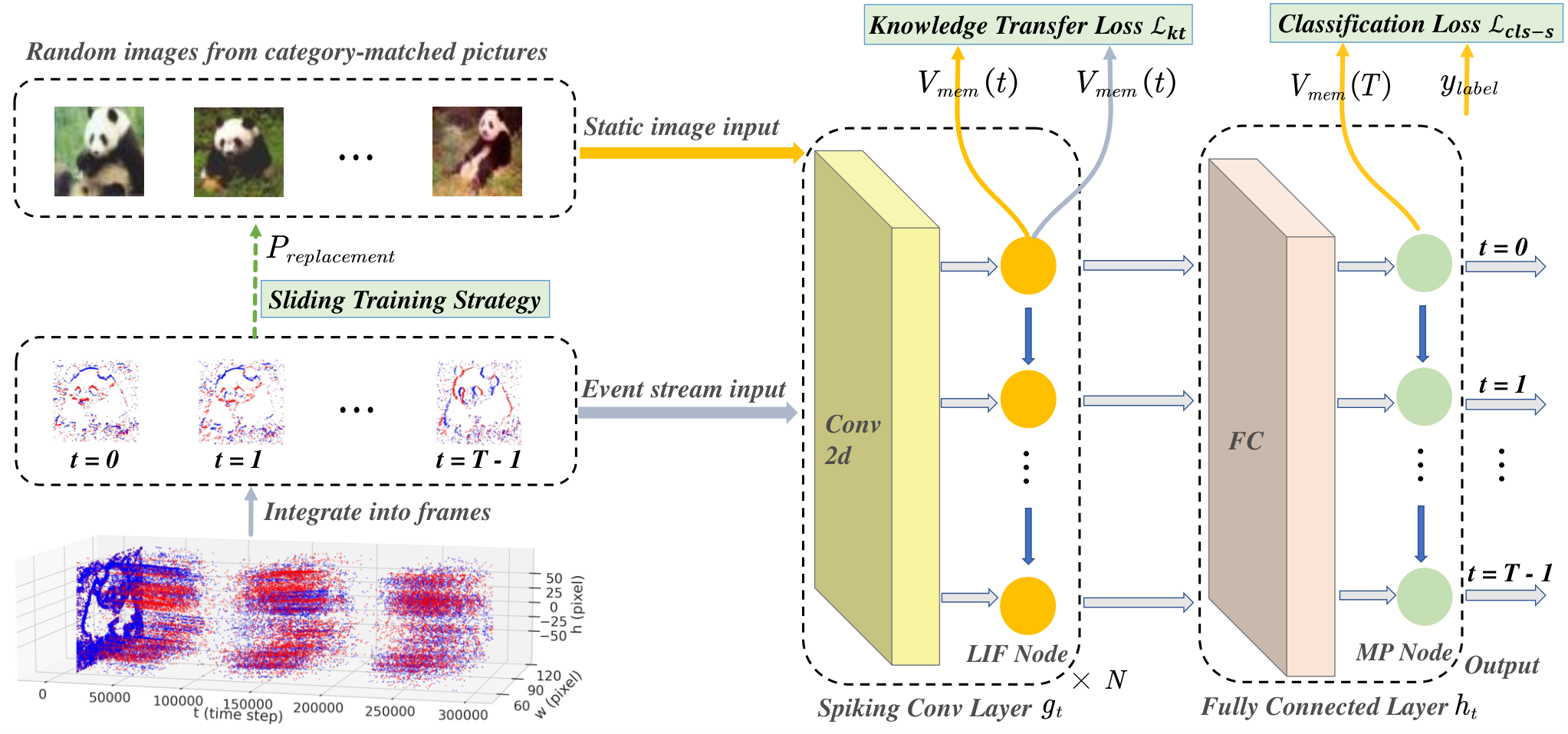
In this paper, the embedding function is modeled by network sharing between the source and target domains, using all layers before the last classification layer, as shown in Fig. 2. At this point, the shared , the optimization objective is to find the satisfied in its hypothetical space :
| (7) |
where and refer to the same data classes in the source and target domains while and mean the data from different classes. The is a metric for judging similarity between two domains; we choose CKA here. CKA is a similarity index to better measure neural network representation similarity introduced by (Kornblith et al. 2019).
| (8) |
where HSIC refers to Hilbert-Schmidt Independence Criterion (HSIC) (Gretton et al. 2005) and can be computed as:
| (9) |
where is the centering matrix , here is an order unit matrix. means trace of matrix.
To compute the CKA, we use a two-stream input paradigm: the inputs come from static image and DVS data, respectively. The closer the value of CKA is to 1 indicates that the two vectors are more correlated. For this reason, we subtract the CKA from 1, minimizing the loss, i.e., maximizing the correlation of the two inputs. We express the samples drawn from the whole data . In this way, domain alignment loss (DAL) can be expressed as
| (10) |
where we use to indicate the value of input after shared parameter function , is brought in to emphasize that here is the output of at time . Two samples are sampled from the same class, expressed by formula . represents the computation of the kernel function of the vectors followed by the computation of CKA by Eq. 8.
Spatio-Temporal Regularization.
Due to the dynamic properties of event data, using only domain alignment loss for spatial feature alignment may miss important information in the temporal dimension. Spatio-temporal regularization provides dynamically learnable coefficients for the domain alignment loss, and such adaptive coefficients ensure specific weight assignments for data features at each time step. To prevent the model from overfitting at a certain time step, we adapt the event data classification loss at each time step (which reflects the contribution of the event frame features to the classification) as the regularization term. In this case, the knowledge transfer loss can be expressed as:
| (11) |
where denotes the learnable coefficient at time step and represents the sigmoid function. For classification loss of event data , we choose the TET loss, which is proven to compensate the momentum loss of surrogate gradient and make SNN have better generalizability (Deng et al. 2022). and are the cross-entropy loss and the mean-squared loss respectively.
We add the knowledge transfer loss and classification loss of the static image as the total classification loss . The total training loss can be expressed as , where and are manually set parameters that determine the ratio of the two types of losses. The knowledge transfer loss not only learns domain-invariant features spatially, but also provides the network with more generalized knowledge by providing appropriate weighting coefficients temporally. This allows the model to adapt fine-grained to event data characteristics.
Sliding Training Strategy
The sliding training strategy aims to modulate the static image input portion of the training process so that the network gradually adapts from relying on domain-invariant features of static images and event data to fully processing event data. Specifically, during the training process, the inputs of static images are replaced by event data with probability, and this substitution probability increases with time steps until the end of the learning phase, by which time event data will replace all static images. Because the substitution process varies over time steps, as if the event data is replacing static images in a sliding time frame, we call it ”sliding training”.
Separately, with denoting index of training batch, denoting total length of training batch, standing for current epoch and denoting maximum training epoch, then the probability of making a substitution could be expressed by the following equation
| (12) |
where is a manual settings epoch for the end of the transfer knowledge loss effects. The value of is usually set to . In the early training phase, domain invariant features are dominant, providing a stable feature learning base for the model. As time advances, the proportion of event data gradually increases and the domain alignment loss gradually decreases. This gradual transition ensures the stability of the model during the learning process and avoids training instability or convergence difficulties that may result from direct or abrupt data switching.
| Dataset | Category | Methods | Architecture | T | Accuracy |
| N-Caltech101 | Data augmentation | NDA (Li et al. 2022c) | VGGSNN | 10 | 78.2 |
| EventMixer (Shen, Zhao, and Zeng 2022b) | ResNet-18 | 10 | 79.5 | ||
| Efficient training | TET (Deng et al. 2022) | VGGSNN | 10 | ||
| TJCA-TET (Zhu et al. 2022) | CombinedSNN | 14 | 82.5 | ||
| TKS (Dong, Zhao, and Zeng 2023) | VGGSNN | 10 | 84.1 | ||
| ETC (Zhao et al. 2023) | VGGSNN | 10 | |||
| Domain adaptation | Knowledge-Transfer (Ours) | VGGSNN | 10 | ||
| CEP-DVS | Efficient training | TET (Deng et al. 2022) | ResNet-18 | 10 | |
| Domain adaptation | Knowledge-Transfer (Ours) | ResNet-18 | 10 | ||
| N-Omniglot | Efficient training | plain (Li et al. 2022a) | SCNN | 12 | 60.0 |
| plain (Li et al. 2022a) | SCNN | 12 | |||
| Domain adaptation | Knowledge-Transfer (Ours) | SCNN | 12 |
Experiments
We conduct experiments on mainstream event datasets: N-Caltech101 (Orchard et al. 2015) and N-Omniglot to evaluate the effectiveness of the proposed method. For another commonly used event dataset, CIFAR10-DVS (Li et al. 2017), since it is 10000 samples taken from 60,000 static images from the training and test sets together, it cannot be ensured that the event data in the manually delineated test set does not overlap with the static images when using the static images to assist training. To avoid this implicit data leakage, we choose the image-event paired CEP-DVS (Deng et al. 2021) dataset as an alternative.
Experimental Settings
We integrate all the event data into frames and then resize to 48x48 for N-Caltech101 and CEP-DVS datasets, and for N-Omniglot dataset, it is resized to 28x28. In terms of network structure, for a fair comparison, we choose VGGSNN (64C3-128C3-AP2-AP2-256C3-256C3-AP2-512C3-512C3-AP2-512C3-512C3-AP2-FC) model with step 10 for N-Caltech101, Spiking-ResNet18 with step 6 for CEP-DVS, and SCNN (15C5-AP2-40C5-AP2-FC-FC) with step 12 for N-Omniglot. For the input encoding strategy, we use direct coding for static images and convert the static image to HSV (Hue, Saturation, Value) color space to minimize the mismatch between the two types of input data. To adapt the dual-channel characteristics of the event data, i.e., positive and negative polarity, we replicate the value channel and then duplicate the static image in equal time-step. All experiments are implemented based on the BrainCog framework (Zeng et al. 2023).
Comparison with the State-of-the-Art
We first evaluate the proposed method on the N-Caltech101 dataset with VGGSNN network and compare the proposed method with NDA (Li et al. 2022c), EventMix (Shen, Zhao, and Zeng 2022b), TET (Deng et al. 2022), TJCA-TET (Zhu et al. 2022), TKS (Dong, Zhao, and Zeng 2023) and ETC (Zhao et al. 2023). The results are presented in Tab. 1. The experimental results demonstrate that the proposed method can achieve state-of-the-art performance compared with existing methods. In particular, with the proposed method, the VGGSNN network can achieve 93.45% accuracy on the N-Caltech101 dataset. The significant performance improvement validates the effectiveness of knowledge transfer.
As for CEP-DVS and N-Omniglot datasets, there are fewer available results. We re-conducted the baseline experiments on these two datasets and compared them with our proposed method. Experimental results show that our proposed method improves accuracy over the original method. For the N-Omniglot dataset, the improvement of accuracy from knowledge transfer is not as significant as the other two datasets, this is because it is a few-shot dataset with only 20 available static images in each class, so the improvement from knowledge transfer is limited.
Ablation Study
In order to verify the effectiveness of the proposed method, in the subsequent ablation experiments, we take the direct training method TET (Deng et al. 2022) as our baseline.
| Network | Methods | Accuracy |
| N-Caltech101 | ||
| VGGSNN | baseline | 79.66% |
| KTL w/o DAL & STR | 84.14% | |
| KTL w/ DAL | 89.31% | |
| KTL w/ DAL & STR | 92.64% | |
| CEP-DVS | ||
| ResNet-18 | baseline | 25.70% |
| KTL w/o DAL & STR | 27.55% | |
| KTL w/ DAL | 29.95% | |
| KTL w/ DAL & STR | 30.50% | |

| Network | Dataset | Methods | Accuracy |
| VGGSNN | N-Caltech101 | w/o sliding training | 83.56% |
| w/ sliding training | 92.64% | ||
| ResNet18 | CEP-DVS | w/o sliding training | 23.70% |
| w/ sliding training | 30.50% |
Knowledge Transfer Loss.
To verify the validity of the domain alignment loss (DAL) and the spatio-temporal regularization (STR) term in the knowledge transfer function, we conduct experiments on N-Caltech101 dataset with VGGSNN. As shown in Fig. 3(a), the baseline, i.e., the TET method, has overfitted at about 100 epochs earlier. Compared to the baseline method, even without employing the knowledge transfer loss in our method, merely using sliding training strategy can achieve certain performance improvement. As it gets better though with the domain alignment loss and spatio-temporal regularization to provide better generalization of the model. In Fig. 3(a), the red line is always at the top in the later training step, indicating that the best results can be achieved with these two terms.
To verify the effect of the spatio-temporal regularization, we also plot the adaptive learning coefficients of the VGGSNN at each time step under the N-Caltech101 dataset. As shown in Fig. 3(b), our dynamically adjusted coefficients are superior to the coefficients that are set to be fixed at each time step, which suggests that spatio-temporal regularization to provide dynamically adjusted coefficients for the domain alignment loss is better able to capture the temporal properties in the data. In addition, the results in Fig. 3(b) show larger coefficients at the first and last time step, which implies that the beginning and ending moment models focus more on domain-invariant spatial information.
Sliding Training Strategy.
We conduct experiments on N-Caltech101 and CEP-DVS to verify the effectiveness of the sliding training strategy, and the results are shown in Tab. 3. The results show that sliding training leads to a more stable performance improvement. It is worth mentioning that in the case of without sliding training, the accuracy of our method is 23.70%, which is slightly lower than the accuracy of the baseline method of direct training strategy, which is 25.70%. This is due to the relatively short training epochs for CEP-DVS, which causes the model to have trouble converging in the face of sudden data switches. Despite this, the addition of sliding training strategy solves this problem well.
Summary of Ablation Experiments.
We show effectiveness of each part of our proposed method with experiments of VGGSNN on N-Caltech101 dataset and the results are shown in Tab. 4. The top line with no added methods is the baseline. It can be seen that without the knowledge transfer loss function, the performance of model decreases a lot. In addition, the sliding training strategy provides a guarantee for stable convergence. Combined with all the approach, our method can achieve the best performance.
| DAL | STR | Sliding training | Accuracy |
| - | - | - | 79.66% |
| ✓ | 82.07% | ||
| ✓ | 84.14% | ||
| ✓ | ✓ | 83.56% | |
| ✓ | ✓ | 90.57% | |
| ✓ | ✓ | ✓ | 92.64% |
Analysis and Discussion
Loss Landscape.
To verify that our method provides SNNs with more generalizability over event data, we utilize 2D loss-landscapes visualization (Li et al. 2018). To this end, we selected the optimal results of the baseline and our method to conduct experiments on N-Caltech101 and CEP-DVS respectively. As depicted in Fig. 4(b) and Fig. 4(d), the lowest loss area becomes flatter compared to Fig. 4(a) and Fig. 4(c), which indicates that the SNN obtains better weights with the knowledge transfer from static images.
Visual Explanations from Deep Networks.
To assess whether our method learns domain-invariant features of static images and event data, and provides helpful information for SNNs about features of event data, we employ grad-cam++ (Chattopadhay et al. 2018) visualization method. Such visualization allows us to understand which local locations of an original image contributed most significantly to the model’s final classification decision. Ideally, static pictures and event data integrated into frames have similar object contour features when they are in the same class. This is well illustrated in Fig. 5, where by introducing knowledge transfer loss, for both static pictures and event data, the network pays attention to the contour features of the category. In particular, the results on event data show that our method helps SNNs to move away from the background of the event data and focus on the features of category itself.

Performance of Our Method on Different Amounts of Event Data.
We conduct a detailed evaluation of our proposed approach on N-Caltech101 dataset using varying amounts of training data, as presented in Fig. 6. Our results show that regardless of training data amount, knowledge transfer loss results in a remarkable performance improvement. This is attributed to the knowledge transfer loss that allows the model to finely adapt to event data features, providing more generalized knowledge to the network.
Conclusion
In this paper, we explore the challenges faced by spiking neural networks when dealing with event-driven data. By using static images to assist SNN training, we improve the generalization ability of the network. Our proposed domain alignment loss and spatio-temporal regularization support knowledge transfer and alleviate the domain mismatch between static and event datasets. Meanwhile, we propose a sliding training strategy to bring greater stability to network training. Experiments on different event datasets show that our method achieves the best performance. In conclusion, this study not only provides new methods for training SNNs on event-driven datasets but also contributes to further development in the field of neuromorphic computing.
Acknowledgments
This work is supported by the National Natural Science Foundation of China (Grant No. 62372453).
References
- Bu et al. (2021) Bu, T.; Fang, W.; Ding, J.; Dai, P.; Yu, Z.; and Huang, T. 2021. Optimal ANN-SNN Conversion for High-accuracy and Ultra-low-latency Spiking Neural Networks. In International Conference on Learning Representations.
- Chattopadhay et al. (2018) Chattopadhay, A.; Sarkar, A.; Howlader, P.; and Balasubramanian, V. N. 2018. Grad-cam++: Generalized gradient-based visual explanations for deep convolutional networks. In 2018 IEEE winter conference on applications of computer vision (WACV), 839–847. IEEE.
- Chen et al. (2020) Chen, G.; Cao, H.; Conradt, J.; Tang, H.; Rohrbein, F.; and Knoll, A. 2020. Event-based neuromorphic vision for autonomous driving: A paradigm shift for bio-inspired visual sensing and perception. IEEE Signal Processing Magazine, 37(4): 34–49.
- Cheni et al. (2021) Cheni, Q.; Rueckauer, B.; Li, L.; Delbruck, T.; and Liu, S.-C. 2021. Reducing latency in a converted spiking video segmentation network. In 2021 IEEE International Symposium on Circuits and Systems (ISCAS), 1–5. IEEE.
- Dayan and Abbott (2005) Dayan, P.; and Abbott, L. F. 2005. Theoretical neuroscience: computational and mathematical modeling of neural systems. MIT press.
- Deng et al. (2022) Deng, S.; Li, Y.; Zhang, S.; and Gu, S. 2022. Temporal efficient training of spiking neural network via gradient re-weighting. arXiv preprint arXiv:2202.11946.
- Deng et al. (2021) Deng, Y.; Chen, H.; Chen, H.; and Li, Y. 2021. Learning from images: A distillation learning framework for event cameras. IEEE Transactions on Image Processing, 30: 4919–4931.
- Diehl and Cook (2015) Diehl, P. U.; and Cook, M. 2015. Unsupervised learning of digit recognition using spike-timing-dependent plasticity. Frontiers in computational neuroscience, 9: 99.
- Dong et al. (2022) Dong, Y.; Zhao, D.; Li, Y.; and Zeng, Y. 2022. An unsupervised spiking neural network inspired by biologically plausible learning rules and connections. arXiv preprint arXiv:2207.02727.
- Dong, Zhao, and Zeng (2023) Dong, Y.; Zhao, D.; and Zeng, Y. 2023. Temporal Knowledge Sharing enable Spiking Neural Network Learning from Past and Future. arXiv:2304.06540.
- Fang et al. (2021a) Fang, W.; Yu, Z.; Chen, Y.; Huang, T.; Masquelier, T.; and Tian, Y. 2021a. Deep residual learning in spiking neural networks. Advances in Neural Information Processing Systems, 34: 21056–21069.
- Fang et al. (2021b) Fang, W.; Yu, Z.; Chen, Y.; Masquelier, T.; Huang, T.; and Tian, Y. 2021b. Incorporating learnable membrane time constant to enhance learning of spiking neural networks. In Proceedings of the IEEE/CVF International Conference on Computer Vision, 2661–2671.
- Fei-Fei, Fergus, and Perona (2004) Fei-Fei, L.; Fergus, R.; and Perona, P. 2004. Learning generative visual models from few training examples: An incremental bayesian approach tested on 101 object categories. In 2004 conference on computer vision and pattern recognition workshop, 178–178. IEEE.
- Gallego et al. (2020) Gallego, G.; Delbrück, T.; Orchard, G.; Bartolozzi, C.; Taba, B.; Censi, A.; Leutenegger, S.; Davison, A. J.; Conradt, J.; Daniilidis, K.; et al. 2020. Event-based vision: A survey. IEEE transactions on pattern analysis and machine intelligence, 44(1): 154–180.
- Gallego et al. (2017) Gallego, G.; Lund, J. E.; Mueggler, E.; Rebecq, H.; Delbruck, T.; and Scaramuzza, D. 2017. Event-based, 6-DOF camera tracking from photometric depth maps. IEEE transactions on pattern analysis and machine intelligence, 40(10): 2402–2412.
- Godet et al. (2021) Godet, P.; Boulch, A.; Plyer, A.; and Le Besnerais, G. 2021. Starflow: A spatiotemporal recurrent cell for lightweight multi-frame optical flow estimation. In 2020 25th International Conference on Pattern Recognition (ICPR), 2462–2469. IEEE.
- Gretton et al. (2012) Gretton, A.; Borgwardt, K. M.; Rasch, M. J.; Schölkopf, B.; and Smola, A. 2012. A kernel two-sample test. The Journal of Machine Learning Research, 13(1): 723–773.
- Gretton et al. (2005) Gretton, A.; Bousquet, O.; Smola, A.; and Schölkopf, B. 2005. Measuring statistical dependence with Hilbert-Schmidt norms. In Algorithmic Learning Theory: 16th International Conference, ALT 2005, Singapore, October 8-11, 2005. Proceedings 16, 63–77. Springer.
- Han, Srinivasan, and Roy (2020) Han, B.; Srinivasan, G.; and Roy, K. 2020. Rmp-snn: Residual membrane potential neuron for enabling deeper high-accuracy and low-latency spiking neural network. In Proceedings of the IEEE/CVF Conference on Computer Vision and Pattern Recognition, 13558–13567.
- Hao et al. (2020) Hao, Y.; Huang, X.; Dong, M.; and Xu, B. 2020. A biologically plausible supervised learning method for spiking neural networks using the symmetric STDP rule. Neural Networks, 121: 387–395.
- He et al. (2020) He, W.; Wu, Y.; Deng, L.; Li, G.; Wang, H.; Tian, Y.; Ding, W.; Wang, W.; and Xie, Y. 2020. Comparing SNNs and RNNs on neuromorphic vision datasets: Similarities and differences. Neural Networks, 132: 108–120.
- Kim and Panda (2021) Kim, Y.; and Panda, P. 2021. Optimizing deeper spiking neural networks for dynamic vision sensing. Neural Networks, 144: 686–698.
- Kornblith et al. (2019) Kornblith, S.; Norouzi, M.; Lee, H.; and Hinton, G. 2019. Similarity of neural network representations revisited. In International Conference on Machine Learning, 3519–3529. PMLR.
- Krizhevsky, Hinton et al. (2009) Krizhevsky, A.; Hinton, G.; et al. 2009. Learning multiple layers of features from tiny images.
- Kugele et al. (2020) Kugele, A.; Pfeil, T.; Pfeiffer, M.; and Chicca, E. 2020. Efficient processing of spatio-temporal data streams with spiking neural networks. Frontiers in Neuroscience, 14: 439.
- Lake, Salakhutdinov, and Tenenbaum (2015) Lake, B. M.; Salakhutdinov, R.; and Tenenbaum, J. B. 2015. Human-level concept learning through probabilistic program induction. Science, 350(6266): 1332–1338.
- Lenz et al. (2021) Lenz, G.; Chaney, K.; Shrestha, S. B.; Oubari, O.; Picaud, S.; and Zarrella, G. 2021. Tonic: event-based datasets and transformations. Documentation available under https://tonic.readthedocs.io.
- Li et al. (2017) Li, H.; Liu, H.; Ji, X.; Li, G.; and Shi, L. 2017. Cifar10-dvs: an event-stream dataset for object classification. Frontiers in neuroscience, 11: 309.
- Li et al. (2018) Li, H.; Xu, Z.; Taylor, G.; Studer, C.; and Goldstein, T. 2018. Visualizing the loss landscape of neural nets. Advances in neural information processing systems, 31.
- Li et al. (2022a) Li, Y.; Dong, Y.; Zhao, D.; and Zeng, Y. 2022a. N-Omniglot, a large-scale neuromorphic dataset for spatio-temporal sparse few-shot learning. Scientific Data, 9(1): 746.
- Li et al. (2022b) Li, Y.; He, X.; Dong, Y.; Kong, Q.; and Zeng, Y. 2022b. Spike calibration: Fast and accurate conversion of spiking neural network for object detection and segmentation. arXiv preprint arXiv:2207.02702.
- Li et al. (2022c) Li, Y.; Kim, Y.; Park, H.; Geller, T.; and Panda, P. 2022c. Neuromorphic data augmentation for training spiking neural networks. In Computer Vision–ECCV 2022: 17th European Conference, Tel Aviv, Israel, October 23–27, 2022, Proceedings, Part VII, 631–649. Springer.
- Li et al. (2023) Li, Y.; Kim, Y.; Park, H.; and Panda, P. 2023. Uncovering the Representation of Spiking Neural Networks Trained with Surrogate Gradient. arXiv preprint arXiv:2304.13098.
- Li and Zeng (2022) Li, Y.; and Zeng, Y. 2022. Efficient and Accurate Conversion of Spiking Neural Network with Burst Spikes. arXiv preprint arXiv:2204.13271.
- Liu et al. (2022) Liu, F.; Zhao, W.; Chen, Y.; Wang, Z.; and Jiang, L. 2022. Spikeconverter: An efficient conversion framework zipping the gap between artificial neural networks and spiking neural networks. In Proceedings of the AAAI Conference on Artificial Intelligence.
- Maass (1997) Maass, W. 1997. Networks of spiking neurons: the third generation of neural network models. Neural networks, 10(9): 1659–1671.
- Messikommer et al. (2022) Messikommer, N.; Gehrig, D.; Gehrig, M.; and Scaramuzza, D. 2022. Bridging the Gap between Events and Frames through Unsupervised Domain Adaptation. IEEE Robotics and Automation Letters, 7(2): 3515–3522.
- Nguyen, Raghu, and Kornblith (2020) Nguyen, T.; Raghu, M.; and Kornblith, S. 2020. Do Wide and Deep Networks Learn the Same Things? Uncovering How Neural Network Representations Vary with Width and Depth. In International Conference on Learning Representations.
- Orchard et al. (2015) Orchard, G.; Jayawant, A.; Cohen, G. K.; and Thakor, N. 2015. Converting static image datasets to spiking neuromorphic datasets using saccades. Frontiers in neuroscience, 9: 437.
- Roy, Jaiswal, and Panda (2019) Roy, K.; Jaiswal, A.; and Panda, P. 2019. Towards spike-based machine intelligence with neuromorphic computing. Nature, 575(7784): 607–617.
- Serrano-Gotarredona and Linares-Barranco (2013) Serrano-Gotarredona, T.; and Linares-Barranco, B. 2013. A 128 128 1.5% Contrast Sensitivity 0.9% FPN 3 s Latency 4 mW Asynchronous Frame-Free Dynamic Vision Sensor Using Transimpedance Preamplifiers. IEEE Journal of Solid-State Circuits, 48(3): 827–838.
- Shen, Zhao, and Zeng (2022a) Shen, G.; Zhao, D.; and Zeng, Y. 2022a. Backpropagation with biologically plausible spatiotemporal adjustment for training deep spiking neural networks. Patterns, 100522.
- Shen, Zhao, and Zeng (2022b) Shen, G.; Zhao, D.; and Zeng, Y. 2022b. EventMix: An Efficient Augmentation Strategy for Event-Based Data. arXiv preprint arXiv:2205.12054.
- Stagsted et al. (2020) Stagsted, R. K.; Vitale, A.; Renner, A.; Larsen, L. B.; Christensen, A. L.; and Sandamirskaya, Y. 2020. Event-based PID controller fully realized in neuromorphic hardware: A one DoF study. In 2020 IEEE/RSJ International Conference on Intelligent Robots and Systems (IROS), 10939–10944. IEEE.
- Stoffregen et al. (2019) Stoffregen, T.; Gallego, G.; Drummond, T.; Kleeman, L.; and Scaramuzza, D. 2019. Event-based motion segmentation by motion compensation. In Proceedings of the IEEE/CVF International Conference on Computer Vision, 7244–7253.
- Sun, Zeng, and Zhang (2021) Sun, Y.; Zeng, Y.; and Zhang, T. 2021. Quantum superposition inspired spiking neural network. Iscience, 24(8): 102880.
- Sun et al. (2022) Sun, Z.; Messikommer, N.; Gehrig, D.; and Scaramuzza, D. 2022. ESS: Learning Event-Based Semantic Segmentation from Still Images. In European Conference on Computer Vision, 341–357. Springer.
- Viale et al. (2021) Viale, A.; Marchisio, A.; Martina, M.; Masera, G.; and Shafique, M. 2021. Carsnn: An efficient spiking neural network for event-based autonomous cars on the loihi neuromorphic research processor. In 2021 International Joint Conference on Neural Networks (IJCNN), 1–10. IEEE.
- Wu et al. (2018) Wu, Y.; Deng, L.; Li, G.; Zhu, J.; and Shi, L. 2018. Spatio-temporal backpropagation for training high-performance spiking neural networks. Frontiers in neuroscience, 12: 331.
- Wu et al. (2019) Wu, Y.; Deng, L.; Li, G.; Zhu, J.; Xie, Y.; and Shi, L. 2019. Direct training for spiking neural networks: Faster, larger, better. In Proceedings of the AAAI Conference on Artificial Intelligence, volume 33, 1311–1318.
- Xing, Di Caterina, and Soraghan (2020) Xing, Y.; Di Caterina, G.; and Soraghan, J. 2020. A new spiking convolutional recurrent neural network (SCRNN) with applications to event-based hand gesture recognition. Frontiers in neuroscience, 14: 590164.
- Zeng et al. (2023) Zeng, Y.; Zhao, D.; Zhao, F.; Shen, G.; Dong, Y.; Lu, E.; Zhang, Q.; Sun, Y.; Liang, Q.; Zhao, Y.; et al. 2023. BrainCog: A spiking neural network based, brain-inspired cognitive intelligence engine for brain-inspired AI and brain simulation. Patterns, 4(8).
- Zhan et al. (2021) Zhan, Q.; Liu, G.; Xie, X.; Sun, G.; and Tang, H. 2021. Effective Transfer Learning Algorithm in Spiking Neural Networks. IEEE Transactions on Cybernetics.
- Zhao et al. (2023) Zhao, D.; Shen, G.; Dong, Y.; Li, Y.; and Zeng, Y. 2023. Improving Stability and Performance of Spiking Neural Networks through Enhancing Temporal Consistency. arXiv preprint arXiv:2305.14174.
- Zhao et al. (2020) Zhao, D.; Zeng, Y.; Zhang, T.; Shi, M.; and Zhao, F. 2020. GLSNN: A multi-layer spiking neural network based on global feedback alignment and local STDP plasticity. Frontiers in Computational Neuroscience, 14: 576841.
- Zhao, Zhang, and Huang (2022) Zhao, J.; Zhang, S.; and Huang, T. 2022. Transformer-Based Domain Adaptation for Event Data Classification. In ICASSP 2022-2022 IEEE International Conference on Acoustics, Speech and Signal Processing (ICASSP), 4673–4677. IEEE.
- Zheng et al. (2021) Zheng, H.; Wu, Y.; Deng, L.; Hu, Y.; and Li, G. 2021. Going deeper with directly-trained larger spiking neural networks. In Proceedings of the AAAI Conference on Artificial Intelligence, volume 35, 11062–11070.
- Zhou et al. (2022) Zhou, Z.; Zhu, Y.; He, C.; Wang, Y.; Shuicheng, Y.; Tian, Y.; and Yuan, L. 2022. Spikformer: When Spiking Neural Network Meets Transformer. In The Eleventh International Conference on Learning Representations.
- Zhu et al. (2018) Zhu, A. Z.; Yuan, L.; Chaney, K.; and Daniilidis, K. 2018. EV-FlowNet: Self-supervised optical flow estimation for event-based cameras. arXiv preprint arXiv:1802.06898.
- Zhu et al. (2022) Zhu, R.-J.; Zhao, Q.; Zhang, T.; Deng, H.; Duan, Y.; Zhang, M.; and Deng, L.-J. 2022. TCJA-SNN: Temporal-Channel Joint Attention for Spiking Neural Networks. arXiv preprint arXiv:2206.10177.
Appendix
Introduction of Datasets
An overview of the datasets used in our experiments is shown in Tab. S1.
CIFAR100.
The CIFAR-100 dataset (Krizhevsky, Hinton et al. 2009) consists of 60,000 color images, each of size 32x32 pixels. These images are divided into 100 classes, with 600 images per class. 50,000 images are used for training and the remaining 10,000 images are used for testing.
CEP-DVS.
The cifar-event paired dataset (CEP-DVS) (Deng et al. 2021) is an event image pairing dataset that contains 10,000 samples in 20 categories. Event samples are generated by capturing motion images of the CIFAR100 dataset displayed on the monitor by an event camera.
Caltech101.
The Caltech101 dataset (Fei-Fei, Fergus, and Perona 2004) contains images from 101 object categories and one background category with a total of 9,145 images and approximately 40 to 800 images for each object category.
N-Caltech101.
The N-Caltech101 dataset (Orchard et al. 2015) is a neuromorphic version of the original Caltech101 dataset. The original data is displayed on an LCD monitor while being captured by using the saccade method of camera movement. N-Caltech 101 removes the ”faces” class from the original dataset to avoid confusion with ”simple faces”. N-Caltech 101 has 100 object classes and one background class, with a total of 8709 samples.
Omniglot.
The Omniglot dataset (Lake, Salakhutdinov, and Tenenbaum 2015) consists of 1,623 handwritten characters from 50 different languages, each with 20 different handwritings, and is a class of small sample handwritten character datasets. 1,200 characters are usually selected as the training set, and the remaining 423 characters as the validation set.
N-Omniglot.
The N-Omniglot dataset (Li et al. 2022a) is the first neuromorphic dataset for few-shot learning using SNNs. The written record of strokes is reconstructed into a video of writing tracks, and then DVS is used to obtain the event records to get the neuromorphic version of Omniglot. Its number of samples is consistent with Omniglot.
Static and Event Data Processing Methods
Processing of Static Datasets.
For all static datasets, we randomly select samples from the training set from the same category as the input event data for the paired input of static images and event data. We resize them in a bilinear interpolation manner to be consistent with the event data. For the Omniglot dataset, the original images are all grayscale. Therefore, we replicate the single-channel images as two-channel to align with the event data dimensions.
Processing of Event Datasets.
The N-Caltech101 and CEP-DVS datasets are uniformly resized to 48 x 48, and the training, validation and testing sets are divided according to 9:1 and 5:3:2 respectively. We use tonic (Lenz et al. 2021) package to integrate them into ten frames, six frames respectively per sample. For N-Omniglot dataset, its size and the way of dividing training and validation sets are the same as the original dataset Omniglot, i.e., 28 x 28 pixel size and 1200 class characters as training set and 423 class characters as the validation set. The event stream is integrated into 12 frames per sample.
| Datasets | Type | Categories | Annotated samples |
| CIFAR100 | static images | 100 | 60000 |
| CEP-DVS | event data | 20 | 10000 |
| Caltech101 | static images | 101 | 9145 |
| N-Caltech101 | event data | 101 | 8709 |
| Omniglot | static grayscale images | 1623 | 32460 |
| N-Omniglot | event data | 1623 | 32460 |
Input Dimension Alignment.
Event data are generated based on rich localized intensity variations in continuous time; therefore, the essence of neuromorphic data describes a sequence of pixel intensity changes over time. Traditional static images use RGB color space, in which all three channels (red, green, and blue) are easily influenced by luminance, i.e., any slight change in luminance will lead to a corresponding change in these three channels. Therefore, it is not intuitive to use RGB to reflect light intensity. Compared with RGB color space, HSV (Hue, Saturation, and Value) color space is more suitable for dealing with light intensity changes. Given this, we choose to convert the static image to the HSV color space to minimize the mismatch between the two types of input data, improving our model’s performance and adaptability. To adapt to the dual-channel characteristics of the event data, i.e., positive and negative polarity, we replicate the value channel and then duplicate the static image in equal time steps. We feed it into the network along with the event data. We replicate directly without additional color space conversion for static image datasets with only a single grayscale channel, such as N-Omniglot.
We conduct experiments with the VGGSNN and ResNet-18 models on the N-Caltech101 and CEP-DVS datasets respectively. We randomly select one of the three RGB channels to represent the without the value channel. The results are shown in Fig. S1. It can be observed that after the conversion to HSV space, the accuracy of the model on both datasets is improved. This demonstrates that using the value channel of HSV color space to represent the light intensity of a static image can better match the characteristics of the event data.
Discussion
Effect of Different Numbers of Static Images on Results.
So far, we have leveraged the full amount of static images. However, a question worth exploring is: How helpful are different numbers of static images in aiding the correct classification of event data? We experimented with VGGSNN on the N-Caltech101 dataset, and the results are shown in Fig. S2. Considering all the event training data, 100% static images mean the same amount of data as the event data. As can be seen from Fig. S2, the more static images used, the richer the generalized features provided to the model, and thus the model performs better. When only 10% of the static images are used to help the model learn the event features, the performance improvement of the model is relatively limited. However, when all the static images are utilized, the performance of the model improves significantly, with the accuracy increasing from 79.66% to 92.64%.
Hyperparameter Settings.
The following parameters need to be set manually in our method: static image classification coefficient , knowledge transfer coefficient and end of the epoch . We set value to 0.5 in all cases. For N-Caltech101 and CEP-DVS, we set to 1.0 and to maximum training epoch respectively. For N-Omniglot, we we set to 1.0 and to . Our approach can be summarized as Algorithm S1.
Utilization and Strengths of CKA.
CKA is a similarity metric that utilizes a kernel approach to measure data similarity in high-dimensional feature spaces. It is increasingly used to compare similarities in network representations, e.g. (Li et al. 2023). In our work, static and event data represent different modalities with inherent domain mismatch. In order to reduce domain distribution differences, we incorporate a distribution difference metric (actually the opposite of the similarity metric) into the loss function. CKA helps to reduce distribution differences between domains by measuring network similarity to align the feature spaces between static and event domains. This alignment is well suited for capturing domain-invariant features, which optimizes the loss function and mitigates network overfitting. It is suitable for dealing with domain adaptation problems, including but not limited to SNN features. With other experimental settings held constant, we replace the similarity metric with maximum mean difference (MMD) (Gretton et al. 2012), a widely used metric in domain adaptation. Tab. S2(a) shows the experiment results to quantify the CKA strengths.
| Similarity Metric | Accuracy |
| - | 25.70% |
| w/ MMD | 26.25% |
| w/ CKA | 30.50% |
| Training Method | Accuracy |
| SEW-ResNet18 | 25.70% |
| Spikformer | 26.15% |
| ResNet18 (Ours) | 30.50% |
Comparison with the High-Performance SNN Works.
We have already compared the work of normal SNN training techniques in Tab. 1, and the comparison illustrates the advantages of our method. Furthermore, we compare the proposed method with two efficient SNN network architectures, Deep Residual SNN (Fang et al. 2021a) and Spikformer (Zhou et al. 2022). We conduct the experiment with these two networks on CEP-DVS dataset. We implement Spikformer according to (Zhou et al. 2022), using 3 transformer encoder blocks and setting the SSA head to 16, keeping other settings consistent with the paper, and the experimental results are shown in Tab. S2(b). As can be seen, a well-designed network structure can still be limited by the small size of the event data, and the results are not so satisfactory. This also illustrates the need to utilize static images to mitigate overfitting from another perspective.
Computational Costs of Knowledge Transfer Training.
Specifically, in order to obtain the final layer features of the static image feature extractor and align the domain distribution, our method requires one additional forward and backward propagation in each iteration. According to our experiments, this extra computation is affordable and improves the performance of the network. In addition, our method requires fewer training iterations and, therefore, achieves better results than existing methods with the same training time, as shown in Fig. S3. It is worth noting that, the additional computation only involves the training stage and there is no additional computational overhead in the inference stage.