Fast and accurate collapse-time predictions for collisionless matter
Abstract
We consider the gravitational collapse of collisionless matter seeded by three crossed sine waves with various amplitudes, also in the presence of a linear external tidal field. We explore two theoretical methods that are more efficient than standard Lagrangian perturbation theory (LPT) for resolving shell-crossings, the crossing of particle trajectories. One of the methods completes the truncated LPT series for the displacement field far into the UV regime, thereby exponentially accelerating its convergence while at the same time removing pathological behavior of LPT observed in void regions. The other method exploits normal-form techniques known from catastrophe theory, which amounts here to replacing the sine-wave initial data by its second-order Taylor expansion in space at shell-crossing location. This replacement leads to a speed-up in determining the displacement field by several orders of magnitudes, while still achieving permille-level accuracy in the prediction of the shell-crossing time. The two methods can be used independently, but the overall best performance is achieved when combining them. Lastly, we find accurate formulas for the nonlinear density and for the triaxial evolution of the fluid in the fundamental coordinate system, as well as report a newly established correspondence between perfectly symmetric sine-wave collapse and spherical collapse.
I Introduction
The cosmic large-scale structure provides a wealth of cosmological information that is accessible by current and forthcoming probes of the galaxy and gas distribution, as well as through maps of the weak lensing signature P. A. Abell et al. (2009) LSST Science Collaboration; R. Laureijs et al. (2011) Euclid collaboration; H. Aihara et al. (2018) HSC collaboration; A. Weltman et al. (2020) SKA collaboration. Fast and accurate theoretical modeling is required in order to retrieve this information and to test the CDM concordance model. One of the most fundamental limitations in the theoretical modeling of cosmic structures is shell-crossing, the crossing of trajectories of collisionless matter. This instant is in particular relevant for the formation of primordial dark-matter halos and is accompanied by extreme matter densities. One central aim of this article is to provide fast and accurate shell-crossing predictions.
Cosmological perturbation theory (CPT) is an indispensable tool in a host of cosmological applications Peebles 1980; Fry 1984; Bernardeau et al. 2002, such as field-level forward modeling for retrieving information about the matter distribution from galaxy surveys Jasche and Wandelt 2013; Kitaura 2013; Wang et al. 2013; Ata et al. 2021 or from the Lyman- forest data Kitaura et al. 2012; Metcalf et al. 2018; Porqueres et al. 2020; Ravoux et al. 2020. Other important applications are to providing initial conditions for cosmological simulations Klypin and Shandarin 1983; Efstathiou et al. 1985; Scoccimarro 1998; Crocce et al. 2006; Michaux et al. 2021, and for pairing CPT predictions with simulations in a variety of hybrid approaches Tassev et al. 2013; Howlett et al. 2015; Feng et al. 2016; Chartier et al. 2021; Kokron et al. 2021; Zennaro et al. 2023; Aricò et al. 2022.
For many applications, however, CPT is employed only for describing perturbatively small departures of the matter density from its steady state, although we do have by now solid evidence that certain implementations thereof can handle much more: indeed, the Lagrangian-coordinates variant of CPT, dubbed Lagrangian perturbation theory (LPT; Buchert and Götz 1987; Buchert 1989; Moutarde et al. 1991; Buchert 1994; Bouchet et al. 1995; Ehlers and Buchert 1997), is able to resolve the shell-crossing singularity to very high precision Rampf and Frisch 2017; Saga et al. 2018; Rampf and Hahn 2021; Schmidt 2021; Saga et al. 2022. This is made technically feasible since the transformation from Eulerian to Lagrangian coordinates acts as a de-singularization transformation Rampf and Frisch 2017; Rampf et al. 2022, turning the density-singularity at shell-crossing into the vanishing of the Jacobian determinant of the transformation—a regular perturbation problem.
Still, LPT converges extremely slowly in general, thereby rendering high-order LPT for many applications as impractical, as large perturbation orders are required to maintain a satisfactory level of precision. For example, to achieve sub-percent-accurate predictions on the shell-crossing time for spherical collapse without resorting to extrapolation methods, LPT at orders is required Rampf 2019. Even worse, LPT exemplifies divergent behavior in voids after some critical time, which is nothing but a mathematical artifact: the radius of convergence of the LPT series is independent of the sign of the local curvature; therefore, the void solution begins to diverge at the instant when a (mirrored) overdensity with sign-flipped curvature collapses Nadkarni-Ghosh and Chernoff 2011; Nadkarni-Ghosh and Chernoff 2013; Rampf and Hahn 2023.
To reduce the impact of some of these shortcomings, there are approaches that combine LPT with predictions from the spherical or ellipsoidal collapse model Kitaura and Hess 2013; Bernardeau 1994; Mohayaee et al. 2006; Monaco et al. 2002; Monaco et al. 2013; Stein et al. 2019; Neyrinck 2016a; Tosone et al. 2021; Monaco 2016; Lippich et al. 2019; however, these strategies do not solve the underlying problem and also come with fairly limited accuracy. Other approaches exploit Padé approximants or Shanks transforms that indeed cure the LPT problems to some extent Tatekawa 2007; Yoshisato et al. 1998; Matsubara et al. 1998; however, to our knowledge, these avenues are typically limited to spherical symmetry (see Ref. Taruya et al. 2022 for an exception).
Recently, the approach of UV completion has been introduced—although also initially limited to spherical symmetry Rampf and Hahn 2023. At the mathematical level, in the UV method one exploits that the LPT perturbation series is a time-Taylor series that comes in general with a finite range of convergence. As with any power- or Taylor series, the range of LPT convergence is determined by the nearest singularity relative to the (temporal) expansion point. Here we note that “singularity” refers to a mathematical property of the asymptotic LPT series which is generically not related to the physical shell-crossing singularity; instead, in the present case, “singularity” refers to the loss of local differentiability after shell-crossing where LPT becomes invalid. With this in mind, the essential idea of the UV completion is as follows: if we know the temporal location of that nearest singularity, e.g. retrieved from suitable extrapolation techniques, we can add a remainder to a truncated LPT series that encapsulates the impact of that singularity, thereby autocompleting the LPT series up to order infinity. By exploiting the asymptotic behavior of the LPT series coefficients at large orders, that remainder turns out to be a critical term of the form related to the loss of differentiability at time , where is the cosmic scale factor, and is a positive non-integer exponent that captures the critical nature of the gravitational collapse, while is the temporal radius of convergence of the LPT series.
In this article, we develop the UV method for the gravitational collapse seeded by three crossed sine waves, the latter being largely representative for high peaks of a smooth random Gaussian density field (see e.g. Doroshkevich 1970; Moutarde et al. 1991; Moutarde et al. 1995; Saga et al. 2018; Saga et al. 2022). We will see that some of the above considerations directly carry over to the 3D case, mostly thanks to the observation that the critical structure of the above remainder is unchanged [although there are in general three distinct pairs of in 3D, each associated with the critical collapse of the three collapse axes in the fundamental coordinate system]. Actually, the form of the remainder also holds for random field initial conditions Rampf and Hahn 2021 and thus, appears to be a generic feature of gravitational collapse. Consequently, we expect that the outlined UV method should be applicable to the case of cosmological initial conditions in the not so distant future.
We test the UV predictions against independent results, the latter are either obtained by applying a computationally expensive nonlinear fitting method Saga et al. 2018, or retrieved from analytical solutions that hold for special setups, namely for exactly symmetric collapse in 2D and in 3D where the initial amplitudes of the crossed sine waves are identical. To our knowledge, these solutions have not been reported in the literature, but we show through a newly established correspondence (verified up to 15LPT) that these sine-wave collapse cases in 2D and 3D are actually related to cylindrical and spherical collapse.
The above mentioned correspondence has been retrieved from normal-form considerations, where the latter comprises the other main focus of this article. Normal-form theory is ubiquitously used in a host of scientific disciplines, such as in asymptotic analysis and catastrophe theory (e.g. Arnol’d 1980; Berry and Upstill 1980; Arnold et al. 1982; DeVille et al. 2008). In cosmology it is particularly useful in the context of cosmic web classification Hidding et al. 2014; Feldbrugge et al. 2014; Neyrinck 2016b and for describing analytically the onset of the post-shell-crossing regime Colombi 2015; Taruya and Colombi 2017; Rampf et al. 2021. In short, normal-form theory attempts to reduce physical models on a geometrical or topological level, such that the physical essence is distilled. In the present case, the approach amounts to spatially Taylor expand the initial data about the shell-crossing location to second order. Within this reduced setup, it turns out that certain space dependencies drop out in the perturbative calculation, thereby enabling us to introduce an auxiliary vector field that requires a normalization condition. After suitable fixing of this condition, the resulting normal-form predictions come with a significantly reduced computational overhead in comparison to standard LPT, and deliver fairly accurate collapse-time predictions.
This article is structured as follows. In the following section, we review the basic equations for collisionless matter in Lagrangian coordinates, and provide an analysis based on LPT at fixed order as well as extrapolated results to order infinity. In Sec. III we develop the UV method for sine-wave initial conditions and discuss details of the required asymptotic input. In Sec. IV we apply a normal-form method to the Lagrangian equations of motion, and in particular discuss in Sec. IV.2 the gauge fixing which is at the heart of the present method. Furthermore, we establish a correspondence between symmetric sine-wave collapse and spherical collapse in Sec. IV.4. Section V is devoted to a general discussion of results, especially related to the shell-crossing time (Sec. V.3), as well as to the triaxial evolution and the nonlinear density (Sec. V.4). An explicit formula for the time of first shell-crossing is provided in Sec. V.5. In Sec. VI we draw our attention to the impact of our results in the presence of a simplified external tidal field. Finally, we summarize and conclude in Sec. VII.
II Fluid equations in Lagrangian coordinates
We employ comoving coordinates , where denotes the physical coordinate, and is the cosmic scale factor governed by the usual Friedmann equations. We label with the initial position of a given matter element at initial time , while denotes its current/Eulerian position at time . Likewise, the Lagrangian displacement field is defined via
| (1) |
Mass conservation is encapsulated in the differential form , where is the matter density, the background density and the density contrast. As long as the flow is single stream, i.e., before shell-crossing, mass conservation is controlled by the Jacobian determinant,
| (2) |
Here we have defined the Jacobian matrix
| (3) |
which plays a central role in the present work. Furthermore, from here on, latin indices denote the three Cartesian components, is the Kronecker delta, and a “” is a partial derivative w.r.t. Lagrangian component . Initially, we have over the whole spatial domain corresponding to a homogeneous density distribution, while the first shell-crossing is achieved at the earliest time and Lagrangian location for which and, as is well known, the density contrast blows up.
With these standard definitions, the Lagrangian evolution equations for collisionless matter elements in a CDM Universe can be written as Peebles 1980
| (4) |
where is the Hubble parameter and a dot represents the Lagrangian (total) time derivative. As is customary in the literature, these equations are supplemented with the statement of vanishing vorticity, i.e., . The conservation of zero vorticity is guaranteed by Kelvin’s circulation theorem; nonetheless, as is well known, transverse displacements in Lagrangian space are required to maintain this zero vorticity condition (see e.g. Buchert 1994; Bouchet et al. 1995; Ehlers and Buchert 1997).
II.1 LPT recursive relations
In standard LPT, the above equations of motion are solved with suitable boundary conditions Brenier et al. 2003a together with the Ansatz
| (5) |
where is the growing mode of linear density fluctuations in CDM, while the ’s are purely space-dependent Taylor coefficients. After suitable divergence and curl operations of (4) and matching the involved powers in , it is by now standard Rampf 2012; Zheligovsky and Frisch 2014; Rampf et al. 2015; Matsubara 2015 to derive the following recursive relations for the th-order displacement divergence and curl part ,
| (6a) | ||||
| (6b) | ||||
| Here, the displacement and -coefficients vanish if any of their upper indices are zero or negative. Furthermore, is a suitably rescaled initial gravitational potential, which is the only physical input for purely growing mode solutions (see, e.g., Michaux et al. 2021 for details), while | ||||
| (6c) | ||||
| (6d) | ||||
| where denotes the Levi–Civitá symbol. We remark that, for simplicity, we have ignored sub-dominant terms in Eqs. (6). These sub-dominant terms have been derived in Ref. Rampf et al. 2022 by means of the Ansatz (5), where it is shown that they are vanishingly small at times when shell-crossing typically occurs, namely at redshifts of , where the precise shell-crossing time depends mostly on the nature of initial conditions Rampf and Hahn 2021. | ||||
The divergence and curl part of the th order displacement are readily obtained from (6), from which one obtains the displacement coefficient using a Helmholtz decomposition,
| (6e) |
Subsequently, one retrieves the truncated displacement field from
| (6f) |
at arbitrary high truncation order . Note that for simplicity we consider in the following sections an Einstein–de Sitter (EdS) cosmological model, where the universe is spatially flat and contains only collisionless matter. In this case, we have , which specifically applies to the Taylor-series representation of the displacement (5) and (6f), which remain exact representations for growing-mode initial conditions until shell-crossing. We remark that our calculations could also be straightforwardly generalized to accommodate less restrictive cosmological setups if required.
II.2 Initial conditions and shell-crossing study in LPT
The truncated displacement field can be readily obtained from the recursive relations (6) once the initial gravitational potential is fixed. In the present paper we consider the gravitational collapse seeded by three crossed sine waves with various amplitudes (see e.g. Moutarde et al. 1991; Moutarde et al. 1995 for early related avenues). Corresponding solutions to large LPT orders have been first investigated in Refs. Saga et al. 2018; Saga et al. 2022. Without loss of generality, we fix the amplitude along the -direction to unity, while we vary only the amplitudes in the directions and keep those “orthogonal” amplitudes below unity; this could be of course easily rectified if needed, e.g., by applying a conformal re-scaling to the initial gravitational potential. In summary, our choice for the initial gravitational potential is
| (7) |
where are not necessarily small amplitudes. With this input, we have generated the first ten LPT coefficients using the above recursive relations. The first two coefficients read
| (8a) | ||||
| (8b) | ||||
which, respectively, reflect the Zel’dovich and 2LPT displacements. Having access to a large number of displacement coefficients, we can estimate the time of first shell-crossing. For this one can employ the truncated displacement defined in Eq. (6f), and search for spatial locations for which the truncated Jacobian
| (9) |
vanishes for the first time, i.e.,
| (10) |
Naturally, the accuracy of the LPT predictions for the shell-crossing time depends on the chosen truncation order, while the “true” shell-crossing time, which we denote with , can be reached within a limiting process (see below for details), i.e.,
| (11) |
Here we should note that, for random initial conditions, also the spatial location of the shell-crossing will depend on the truncation order Rampf and Hahn 2021. However, for the present initial conditions (7), it is easy to see that the shell-crossing location is fixed and occurs precisely at
| (12) |
and, of course, at -periodic repetitions along .
An accurate estimation of from the limit in (11) requires a precise asymptotic form of the LPT expansion, which is, however, a priori unknown. To remedy the problem, Refs. Saga et al. 2018; Saga et al. 2022 proposed to retrieve from a nonlinear fitting procedure based on the model
| (13) |
To be precise, one first determines from the condition (10) for varying truncation orders , and then uses this input in (13) to fix the unknown fitting coefficients and . We have done so by performing a nonlinear fit between LPT orders ; the results of this are shown in Fig. 1 for various amplitudes (solid lines), and compared against fixed-order LPT estimates (dotted markers). The overall performance of the nonlinear fitting procedure has been tested against very accurate numerical simulations in Refs. Saga et al. 2018; Saga et al. 2022 by using ColDICE Sousbie and Colombi 2016. Based on these tests we take the shell-crossing estimates from (13) as a benchmark for the following sections.
In Fig. 1 it is seen that first-order LPT only delivers an exact shell-crossing prediction when are exactly zero—this is of course a well-known result reflecting that the Zel’dovich approximation becomes exact for one-dimensional collapse Novikov 1969; Zentsova and Chernin 1980; McQuinn and White 2016, which is here embedded into three-dimensional space. Departing just slightly from this case while the orthogonal amplitudes are still sufficiently small, one achieves so-called quasi-one-dimensional collapse where low-order LPT delivers fairly accurate results Rampf and Frisch 2017; Saga et al. 2018; Saga et al. 2022. By contrast, for larger orthogonal amplitudes which is related to more generic collapse Bardeen et al. 1986, low-order LPT struggles to accurately predict the shell-crossing time, which can also be seen in Fig. 1. In section III we will see that this weak performance for generic collapse originates from evaluating the LPT displacements in the vicinity where singular (non-differentiable) behavior occurs.
II.3 Jacobian matrix at shell-crossing location

In the previous subsection, we have determined the shell-crossing time by demanding the vanishing of the Jacobian determinant , which indeed is a sufficient condition. However, it is often instructive to consider instead the vanishing of the elements of the Jacobian matrix. Specifically, for this one considers the Jacobian matrix with components , and diagonalizes it into the coordinate system along the fundamental axes (see e.g. Zel’dovich 1970; Doroshkevich 1970; Rampf and Hahn 2021 for details), such that, for fixed , we have
| (14a) | ||||
| Actually, for the initial condition (7), the Jacobian matrix is already in diagonal form at shell-crossing location ; thus, no diagonalization is required in the present case and we simply have , where underlined indices are not summed over. The respective elements read | ||||
| (14b) | ||||
| (14c) | ||||
| (14d) | ||||
up to order 2LPT, where we remind the reader that we have set the initial amplitude in the direction to unity. At times , these diagonal elements turn into identities, reflecting the statement of initial (quasi-)homogeneity (see e.g. Rampf and Buchert 2012). Evolving to later times, shell-crossing occurs when any of these elements vanishes for the first time, which generically occurs first along a single axis Doroshkevich 1970.
In our setup with the assumed ordering , it is easy to see that the first shell-crossing happens when the first diagonal element, , vanishes for the first time. Consequently, in what follows we draw our attention mostly on the evolution of .
In Fig. 2 we show the temporal evolution of for several choices of initial amplitudes . Colored lines denote truncated solutions in LPT, while the black dotted line reflects the result of the UV-completed LPT series to order infinity (see section III for details). Vertical dashed lines resemble the shell-crossing prediction at order infinity, based on exploiting the nonlinear model fit (see Fig. 1 and eq. 13); we remark that the UV-completed result is independently derived and thus does not need as an input. Finally, the regime of LPT convergence is marked in Fig. 2 with a gray shading, which we have determined using the asymptotic methods discussed in section III.
In the top-left panel of Fig. 2, we show the highly symmetric case , dubbed “S3D”, where the range of LPT convergence is terminated precisely at the time of first shell-crossing, i.e., for S3D we have where is the LPT radius of convergence (see further below for details). This loss of convergence (which also persists in the symmetric two-dimensional collapse case with and ; see bottom-left panel in Fig. 4), has been already noted before in the literature Saga et al. 2018; Saga et al. 2022, where numerical evidence has been obtained that the velocity blows up at shell-crossing. Later in section IV we will see that this congruence between the time of LPT convergence and of the shell-crossing time can be understood by means of the exact parametric solution for spherical collapse.
A general comment can be made about all LPT solutions for , since they all predict correctly the existence of the first shell-crossing—albeit the precise estimate on the shell-crossing time varies by quite a lot and is dependent on the initial amplitudes (see also Fig. 1), as frequently noted in the literature (see e.g. Saga et al. 2018; Rampf and Hahn 2021; Saga et al. 2022). Another interesting observation is with regards to the post-shell-crossing regime, where all LPT solutions pivot far into the negative regime of , indicating that the collapsed structure along the first fundamental axis continues to expand and thus structures dissolve again. Also this pathological behavior of LPT has been already observed in the literature. Having this in mind, observe that the UV predictions follow a distinct trend after the first shell-crossing: the primary axis recollapses. We note that this is a somewhat pathological behavior since the presently employed UV method (and of course also LPT) break down after the first shell-crossing.
Finally, we remark that one could also exploit the nonlinear fitting procedure from the previous section to retrieve estimates of the temporal evolution of at order infinity (cf. eq. 13). For this one first evaluates for varying truncation orders . Then, the corresponding estimate at order infinity, dubbed , is obtained through a nonlinear model fit based on , where the coefficients are again fitting parameters. We have tested this nonlinear fitting procedure which works fairly well for predicting the temporal evolution of , however only within the expected range of LPT convergence and at vastly increased computational costs. Therefore, in what follows we do not consider the nonlinear fitting procedure for presenting the evolution of the eigenvalues .
III UV completion
We have just seen that fixed-order LPT fails to accurately predict the shell-crossing time, especially for collapse scenarios that deviate strongly from quasi-one-dimensionality. In the following subsection we develop a much faster converging method for sine-wave initial conditions that alleviates some of the weaknesses of LPT. This method, called UV completion, was recently introduced in Ref. Rampf and Hahn 2023, however only applied to the simplified case of spherical symmetry—which we rectify in what follows (the case of random-field initial conditions is discussed in Sec. VII). Then, in Sec. III.2, we explore the UV method by means of the primary Jacobian matrix element that triggers shell-crossing. Finally, results on the shell-crossing time are discussed in Sec. III.3.
III.1 UV method
Given that the shell-crossing time is determined by the vanishing of a certain element of the Jacobian matrix, , we find it convenient to develop the UV method here by means of gradients of displacements,
| (15) |
where the displacement coefficients are determined through the recursive relations (6). We also remind the readers that we assume, for simplicity, an EdS cosmological model for which , although this could be easily rectified to a CDM Universe (and beyond).
The general idea of the UV method is as follows. Suppose we know some intrinsic properties of the fully nonperturbative displacement field, denoted with , which captures the critical behavior of the gravitational collapse deep in the ultra-violet regime. Then the UV method simply suggests to split off this nonperturbative term from the infinite LPT series (15),
| (16) |
(see eq. III.1 for the result in explicit form). Here, is the truncated Taylor series of about up to truncation order ; this term is needed to circumvent double counting of certain low-order coefficients.
To be more specific about how the method works, let us examine the UV completion just for the displacement gradient since this is the physically significant element for determining the first shell-crossing, considering the assumed ordering ; the application to the other displacement gradients is analogous and discussed in Sec. V.4. Suppose that the displacement gradient behaves far in the UV as
| (17) |
where is a constant, is a critical exponent (if it is a positive non-integer), while denotes a critical temporal value where the displacement gradient is not infinitely differentiable in time. The latter is a classical instance of a mathematical singularity, since all Taylor coefficients with will blow up at . Here, “” denotes the floor function that outputs the integer value of a real-valued input. Note that each displacement gradient comes in general with a distinct pair of and (see Sec. V.4); we keep the present simplified notation for ease of exposition.
Now, investigating subsequent ratios of Taylor coefficients of the Taylor-series representation of (17), and comparing them against the ratios obtained from the displacement series (15), one can deduct that the large-order asymptotic behavior of (15) is precisely encapsulated by (17), provided that the following equality holds for
| (18) |
at shell-crossing location (see e.g. Domb and Sykes 1957; van Dyke 1974; Rampf 2019; Rampf and Hahn 2023 for further details and related avenues in various contexts). In other words, if the ratios settle into a linear relationship in for sufficiently large , then we can exploit Eq. (18) to determine the two unknowns and from a simple linear fit/extrapolation. We remark that, mathematically, if the linear extrapolation would output , then the asymptotic behaviour of the displacement would be instead of (17); see e.g. Ref. van Dyke 1974 for details.
In Fig. 3 we determine and with the above outlined strategy. Specifically, in the left panel we draw the so-called Domb–Sykes plot of subsequent ratios of as a function of , obtained from the first 10 LPT coefficients based on the initial condition (7) [faint markers and lines denote normal-form results discussed in section IV]. It is seen that, as long as are sufficiently large (see further below for comments), then the ratios of displacement coefficients settle into a linear behavior for sufficiently large orders, justifying a linear extrapolation to the -intercept, from which one can read off and . In the present case, we used the coefficients between the LPT orders for the involved linear fit, and the resulting extrapolations for an exemplary set of amplitudes are shown as dashed lines in the left panel of Fig. 3.
The right panel of Fig. 3 summarizes the estimated results for and over a wide range of initial amplitudes . Only a few limiting cases shown in this panel can be related to known results in the literature: Specifically, as we will see shortly, the highly symmetric case with is directly related to the classical spherical collapse problem by exploiting a newly established correspondence (verified at 15LPT), from which one retrieves the prediction and ; see section IV for details about this nontrivial finding. By contrast, with the outlined linear extrapolation technique up to order 10LPT, we find and , which deviate from the analytical prediction by % and %, respectively. A similar correspondence can also be exploited to retrieve the shell-crossing time for the exactly symmetric 2D collapse case with and , where we find (see App. A for details); by contrast, the linear extrapolation with 10LPT input delivers which deviates from the previous result by . Another example where we know is for one-dimensional collapse where : This is the case where a one-dimensional flow is embedded in 3D, for which the Zel’dovich solution is analytic for all real-valued times. Thus, for exactly one-dimensional collapse theoretically, but our outlined method at order 10LPT predicts instead (recall that in this regime the used linear extrapolation is strictly speaking not justified; cf. above discussion). Still, as we show below, even with these approximate or occasionally even crude estimates, the UV completion clearly outperforms LPT.
Within the UV approach, the results for and serve as the sole input needed to determine the critical term (17), which is then used to complete the truncated LPT series to order infinity. The only remaining task to do is to fix the constant appearing in (17), which is done by demanding that the series coefficient of the Taylor series of (17) is identical with the LPT coefficient at truncation order . These considerations then lead directly to the UV completed result
| (19) |
where involves a generalized binomial coefficient. We note that and are in general dependent on the selected components of , but here and in the following we suppress this dependency for notational ease; see section V.4 (or App. B.3) for details.
Equation (III.1) can be directly used to determine the UV-completed displacement at shell-crossing location. For example, for and the present choice of initial data (7), we have
| (20) |
(the limiting cases or are well behaved), relevant for the first Jacobian element . We remark that, instead of using the outlined large-order extrapolation method to retrieve and , we also found analytical expressions solely derived from considerations at order 3LPT, that lead to very accurate UV-completed results; see Sec. V.5 for an explicit formula for the shell-crossing time, and App. B.3 for further results.
Finally, if required, one can obtain the UV-completed displacement from the UV-completed displacement gradients (III.1) using a standard Helmholtz decomposition,
| (21) |
where from here on. In the following we will mostly focus on the analysis of the first Jacobian element, as it is physically the most relevant one for the ordering . See section V.4 for results related to the triaxial evolution, which is in particular relevant for relating the nonlinear density to its linear counterpart.
III.2 Evolution for the first Jacobian element
Here we analyze the resulting UV predictions for the temporal evolution of the first diagonal element of the Jacobian matrix at shell-crossing location (for the present ICs: also an eigenvalue of that matrix), defined with
| (22) |
where can be straightforwardly determined from Eq. (III.1) for given truncation order . In Fig. 4 we show, for various amplitudes, the results for the UV-completed diagonal element. Solid [dashed] lines denote UV-completed [LPT] results for the truncation orders . As before, positive times reflect the collapse case, but here we have also added the negative time branch, which can be associated with the void evolution Nadkarni-Ghosh and Chernoff 2011; Rampf and Hahn 2023: Indeed, gravity acts effectively as a repulsive force when the arrow of time is reverted, which physically amounts to follow the evolution of underdense regions. This last statement makes in particular sense when considering the symmetric sine-wave collapse shown in the top-left panel of Fig. 4; there we have also added the exact parametric solution (black dotted lines) which can be retrieved from a correspondence with the spherical collapse model (see section IV for details).
For arbitrary initial amplitudes, we can make two general observations: (1) for negative times beyond the range of LPT convergence, the UV methods exemplify no pathological behavior as seen in the LPT solutions; and (2) convergence in the collapse case appears to be vastly accelerated within the UV method as compared to LPT. The last statement is also supported by the independent prediction of the shell-crossing time (vertical gray-dashed lines) through the nonlinear fitting method based on Eq. (13), which agrees well with the UV estimates for the shell-crossing time (see also next section).
Finally, we remark that the critical term appearing in the UV predictions (III.1) becomes complex for , since the critical exponent is a positive non-integer. Clearly, this complexification is an artifact stemming from the considered mathematical model; we leave a post-shell-crossing analysis of the UV method as future work. For the time being and for reasons of illustration, we do not terminate the UV (neither the LPT) results beyond the time of validity, and instead take implicitly their real parts.
III.3 UV results for the shell-crossing time
To elucidate in detail the UV predictions for the shell-crossing time, denoted with for various UV truncation orders , we determine numerically the vanishing of the element of the Jacobian matrix, i.e.,
| (23) |
Here, the required UV result is determined through Eq. (III.1) that needs and as sole input for which, as described above, we use the linear extrapolation results between LPT orders 7-10 (see Fig. 3). Figure 5 summarizes the respective findings and compares them against the shell-crossing predictions from the nonlinear fitting procedure based on Eq. (13). Specifically, the top panel shows as a function of varying amplitudes, while the various subpanels display the relative difference for the UV truncations . Generally, the agreement between the various UV estimates conforms closely to , with a relative difference in the lower permille regime. For 3UV, the shell-crossing time appears to be slightly overestimated (cf. evolution of shown in Fig. 4), while 4UV and 5UV deliver almost equivalent predictions. We note that this slight dependence on the UV truncation order is generically expected for asymptotic methods, and has been already observed in Ref. Rampf and Hahn 2023 for the simplified case of spherical symmetry.
| collapse | ||||||
|---|---|---|---|---|---|---|
| 1D | ||||||
| Q1D | ||||||
| S2D | ||||||
| S3D |
But which of the shown predictions, including the ones from the nonlinear fitting method, are the most trustworthy? Except for a few special collapse cases, this question is difficult to address rigorously. Table 1 summarizes the shell-crossing estimates from various methods, and compares them against the theoretical predictions (dubbed ) for some limiting collapse cases. Specifically, for quasi-one-dimensional (Q1D) collapse, the theoretical prediction is given by Ref. Rampf and Frisch 2017 for which we also know that LPT delivers highly accurate results Saga et al. 2018; Saga et al. 2022. It is seen that, for Q1D, all of the methods agree to high precision on the shell-crossing time, which is expected. Another special case is for the symmetric 2D collapse (S2D) with and for which we find , obtained by exploiting a correspondence to cylindrical collapse (see App. A). For the special case of S2D, the UV and nonlinear fitting methods deviate from the aforementioned result by only and respectively, while 10LPT disagrees by . Finally, for perfectly symmetric 3D collapse (S3D) with , we know the shell-crossing time actually exactly, namely , obtained by exploiting a conjectured correspondence with spherical collapse (section IV). By contrast, the UV and nonlinear fitting methods deviate from the theoretical prediction by and , respectively, while 10LPT mispredicts the result by . Here, it is intriguing to recall that all shown results rely on the same identical “input”, which in the present case is 10LPT.
The accuracy of the UV method could be refined when the linear extrapolation is performed at higher LPT orders than 10LPT. This statement can be verified for S3D for which we exploit the correspondence to spherical collapse (see next section)), thereby providing us trivial access to very high LPT orders (Ref. Rampf 2019 determined solutions up to 1000LPT): For example, using 18-20LPT as input for the linear extrapolation needed to determine the unknowns of the 5UV method, we find which deviates from the theoretical prediction by only —this is more than a fourfold reduction of the error in comparison to the 10LPT result. By contrast, the nonlinear fitting method does not benefit much from including 20LPT solutions, for which we predict a deviation from the theoretical prediction of —a minuscule improvement by a factor of about 1.4 in comparison to the above estimate at order 10LPT.
In summary, based on the above discussed special collapse cases, the nonlinear fitting method appears to be slightly more accurate than the UV method, at least when the input for the extrapolations is retrieved up to order 10LPT. Note however that the UV method requires a simple linear fitting procedure which is significantly cheaper computationally than the nonlinear fitting method (e.g., about 100 times faster for predicting for ). The UV method can be even further accelerated in computational speed: one avenue of this is discussed in the following section, while yet another one is outlined in Sec. V.5 that comes with an accurate formula for the shell-crossing time; see also App. B.3 for more explicit formulas.
IV Normal-form considerations
We have just seen that the UV method delivers much better collapse predictions than LPT. Now we introduce another technique, which is in principle independent from the UV approach. The basic idea motivated here is related to so-called normal forms, which in essence involve physically motivated Taylor-expansions about spatial locations. In the past, similar normal-form techniques have been developed, especially in the context of catastrophe theory Arnol’d 1980; Berry and Upstill 1980; Arnold et al. 1982, where such considerations are performed at critical points where certain derivatives vanish (cf. Morse theory); see e.g. Refs. Magner and Arita 2017; Feldbrugge et al. 2018; Offen and Ober-Blöbaum 2021 for recent applications in various contexts. Related normal-form techniques have been also applied in Refs. Colombi 2015; Taruya and Colombi 2017; Rampf et al. 2021 to investigate analytically the onset of the post-shell-crossing regime.
Below we develop a normal-form technique with the primary aim to accurately predict the triaxial evolution of the fluid collapse—in a computationally faster manner as compared to LPT. As we will see, this involves spatial expansions of the initial data around the shell-crossing location. Preliminary considerations and results are discussed in the following subsection, while a renormalization technique is motivated in Sec. IV.2. In Sec. IV.3 we apply the renormalized normal-form method to establish a correspondence between symmetric sine-wave collapse and spherical collapse. Then, in Sec. IV.4 we explore the normal-form method for sine-wave collapse for arbitrary amplitudes, as well as pair it with the UV method. Afterwards, results are discussed in Sec. V.
IV.1 Normal-form reduction
The central idea of the considered normal-form technique is as follows. Instead of employing the initial condition
| (24) | ||||
| for determining the LPT displacement, we use its normal form defined with | ||||
| (25) | ||||
where here and in the following, quantities or fields that contain the index “N” are based on this normal-form reduction. Intuitively, Eq. (25) is nothing but the second-order spatial expansion of the initial condition (24) about the shell-crossing location (we discard the zeroth-order Taylor coefficient as it has no relevance for determining the displacement field).
Solving the Lagrangian equations of motion (4) with the normal-form initial condition (25) is straightforward. In fact, the Ansatz for the normal-form displacement is equivalent with the one from standard LPT, i.e., in the EdS case. Even more, the recursive relations (6) for the divergence- and curl-part of the displacement are also valid upon the replacement . Note that one crucial ingredient needed to retrieve for is altered in comparison to standard LPT, which we discuss in section IV.2.
As in the standard LPT analysis, the first-order displacement in normal form is simply obtained from
| (26) | ||||
| which implies the corresponding Jacobian matrix at first order | ||||
| (27) | ||||
It is illuminating to notice that this matrix agrees exactly with as obtained in standard LPT (see Eqs. 14). In other words, at the present order, the predictions of the normal-form reduction resemble exactly the standard LPT predictions at shell-crossing location. We will shortly see that this exactness is in general lost at higher perturbative orders. Still, the shell-crossing predictions in normal form quite accurately resemble those of the standard LPT approach. Thus, in much sense, the essence of the gravitational collapse is encapsulated correctly in the normal-form reduction.
While the Jacobian matrix in standard LPT depends on the Lagrangian coordinate, the Jacobian matrix in normal form is directly evaluated at the shell-crossing location . Thus, trivially, the normal-form reduction has no coordinate dependence, at least not at the level of the Jacobian matrix (the normal-form displacement must depend on , otherwise at all times which is unphysical). This is however not really a drawback but instead comprises a vast simplification of the system, especially when the normal-form method is applied to arbitrary high perturbation orders: Indeed, as we will see shortly, the output of the LPT recursive relations in the normal-form case are simply space-independent numbers, and only a function of the initial amplitudes , thereby drastically reducing the computational overhead of evaluating the LPT recursive relations.
IV.2 Normalization of normal-form displacement
Let us comment now on the details of how to determine the normal-form displacement, which is at the heart of the present method. As mentioned above, the recursive relations (6) also hold but come with significant simplifications in the normal-form case (see also Eq. 35). Specifically, since the normal-form initial condition (25) is, by construction, only twice differentiable in the space variable, it is easy to see that the displacement divergence, denoted with , is space independent and thus depends only on the initial amplitudes. Furthermore, by a similar argument of “running out of derivatives,” it can be shown that the Lagrangian curl of the normal-form displacement, dubbed , is vanishing at each perturbation order.11 1 The same is actually also true for the standard LPT result at , at least for the initial condition (24) and in the absence of external tidal fields. Summing up, at each perturbation order , we have the following simplification for the normal-form displacement divergence and curl at shell-crossing location,
| (28) |
where we remind the reader that is a space-independent coefficient and determined through the recursive relation (6a) upon the replacement . In the normal-form approach, the displacement field is constructed solely from its divergence part through an adapted Helmholtz decomposition defined with ()
| (29) |
where we have introduced the auxiliary vector field that is constrained by . This constraint is needed to ensure that the displacement divergence at the present perturbation order remains unaltered (which otherwise would lead to inconsistencies). At the same time, it is easily seen that a large class of vector fields satisfy this constraint, and in the following we call different choices for a normalization condition.
In principle, the normalization condition of the normal-form displacement could vary at distinct perturbation orders. However, we found that by just applying the same normalization condition to all orders already comes with an excellent performance and, for the limiting case of symmetric collapse, even to an exact correspondence (verified to order 15LPT, see the following section). Specifically, in what follows we demand for all , and set
| (30) |
where we have assumed that the Jacobian matrix in LPT has been already diagonalized (not needed in the present case since the solution is already diagonal at shell-crossing location for sine-wave initial conditions). In words, this normalization condition ensures that the normal-form Jacobian matrix coincides exactly with the Jacobian matrix at shell-crossing location to second order in standard LPT. For the present choice of initial condition (24), this vector field takes the form
| (31) |
As we will see shortly, this second-order normalization condition leads to accurate predictions for the triaxial collapse. We remark that we have also tested a third-order normalization condition, where we applied Eq. (30) at second order followed by a third-order matching condition against 3LPT. However, the normal-form predictions with third-order normalization condition compared just slightly better without really justifying the additional layer of complexity, therefore in what follows we consider only the second-order fixing for simplicity.
IV.3 Symmetric sine-wave collapse and spherical collapse
As the simplest application of the above normal-form method, let us limit ourselves to the perfectly symmetric collapse case “S3D” with . Related to that we demonstrate here two results, namely that
-
the normal-form method based on the initial condition
(32) predicts the identical shell-crossing time as obtained in standard LPT model based on
(33) and that
-
the normal-form displacement for S3D agrees exactly with the LPT displacement in the case of spherical symmetry.
As a by-product of these two findings, we establish a so far unknown correspondence between symmetric sine-wave collapse and spherical collapse. This correspondence leads to a theoretical prediction of the shell-crossing time for symmetric sine-wave collapse, thereby providing a novel and nontrivial prediction related to the cosmic fluid equations in 3D.
Let us begin with the first task for which we remind the reader that the normal-form method requires choosing a normalization condition for the corresponding displacement field. For this we employ (30) which implies (31). Actually, for perfectly symmetric collapse in 3D with , Eq. (31) reduces to , and thus
| (34) |
We remark that the computation of the normal-form kernels for through the recursive relation (6a) simplifies in comparison to the sine-wave model, since, for ,
| (35) |
Plugging this together with into (6a) yields a vastly simplified recursive relation for the normal-form displacement; the first terms of the solution read
| (36) |
It is easy to see that the resulting Jacobian matrix, , coincides with the one for the sine-wave model at shell-crossing location (Eq. 14 for ), which we have explicitly verified up to the 15th order in perturbation theory, thereby establishing the direct link between normal-form method and standard LPT for S3D.
Next we consider the second task which is establishing the connection to spherical collapse. For this, Refs. Rampf 2019; Rampf and Hahn 2023 have shown that spherical collapse can be realized with LPT in a Cartesian coordinate system when the corresponding Jacobian matrix is diagonal with identical entries. In that case the Lagrangian equations of motion (4) can be solved with the refined Ansatz ()
| (37) |
where is a free parameter that amounts to an effective curvature of a spherical region within an otherwise spatially flat universe. The scalar coefficients in (37) are determined by the following recursive relations Rampf 2019
| (38) |
where is zero if the perturbation index is zero or negative. Using this one directly obtains the displacement in spherical symmetry
| (39) |
up to . Evidently, with the choice , this low-order result agrees exactly with the normal-form result (36). Actually, this agreement holds at any order in perturbation theory, since the recursive relations in the normal-form and spherical case (for ) imply an identical displacement; cf. Eq. (IV.3) against Eq. (6a) with the simplification (35). Furthermore, since (37) is an exact representation of the parametric solution for spherical collapse within the disc of convergence (see also Refs. Rampf 2019; Rampf and Hahn 2023), we can conclude that also the normal-form method reproduces this result.
Thanks to the so-obtained correspondence, we can test our UV and normal-form predictions for S3D against the parametric solution for spherical collapse, which is
| (40) |
where is conformal time, while is a constant scalar curvature which is a free parameter within the model (see e.g. Rampf and Hahn 2023 for details). On a technical level, to retrieve the temporal evolution of as shown in the left panel of Fig. 4, we set for , and then plot parametrically over . Similarly, to determine the nonlinear density contrast as a function of using spherical collapse, one plots parametrically over . See Sec. V and in particular Fig. 10 for a direct comparison between spherical collapse and S3D by means of the nonlinear density contrast.
We remark that a similar correspondence persists also for exactly symmetric two-dimensional collapse which is achieved for and ; see App. A for details.
IV.4 Normal-form displacement for triaxial collapse
Now we analyze the normal-form techniques for arbitrary initial amplitudes , for which we choose again the second-order normalization condition (30). With this condition and by using (29) as well as the recursive relation (6a) upon the replacement , it is straightforward to determine the normal-form displacement
| (41) |
up to order , where and is given in Eq. (31). For the following analysis, we have generated ten LPT coefficients in normal form (which takes only a fraction of a second on a contemporary single-core machine), which is sufficient for the main purpose of this article, namely developing methods for fast and accurate shell-crossing predictions.
Most tools and methods from the previous sections still apply in the normal-form case employing (41), however generally the resulting predictions can vary slightly. In particular, as mentioned above, the displacement field in normal form is retrieved from the recursive relations (6) together with the adapted Helmholtz decomposition (29), leading to
| (42) |
(as before valid for an EdS universe), up to truncation order . We remark that the coordinate dependence in (42) is somewhat of residual nature, as it is technically needed for applying spatial gradients in order to construct the Jacobian matrix; implicitly, Eq. (42) is defined locally about . From here on, results based on (42) are denoted with “LPT-N.”
Determining the time of shell-crossing is straightforwardly achieved in the normal-form method, by solving for
| (43) |
where is defined as in (9) but with the replacement , and is the shell-crossing time at truncation order . Also, the nonlinear fitting procedure discussed earlier can be applied (cf. eq. 13),
| (44) |
where is the normal-form estimate of the shell-crossing time at order infinity, and are fitting coefficients.
Even more, the UV techniques of section III apply also to the normal-form method—thanks to an asymptotic behavior of the normal-form displacement that is very similar to the one in standard LPT; cf. faint lines in Fig. 3 but see also the related discussion in section V. Specifically, the normal-form- and UV-completed displacement is
| (45) |
where . Here we note that the unknowns and are actually identical for the three components ; see below for comments.
Equation (IV.4) can be straightforwardly used to determine the UV completed normal-form prediction, which we abbreviate in the following with “UV-N.” For example, for the truncation order , the UV-N displacement reads
| (46) |
which does not coincide with the corresponding 3UV prediction (20) in LPT; see the following section for a discussion of related results.
Lastly, we comment on the technical subtlety that and are identical unknowns for the gradient displacements , and . To understand why this is the case (and not for the UV model based on eq. III.1), recall that and are determined through limiting considerations based on subsequent ratios of coefficients for large orders . But since the normal-form displacement has identical spatial dependence for (cf. eq. 29), it is easy to see that, for fixed components , we have
| (47) |
where are constants in space and time that are determined through the recursive relations (6a) adapted to the normal-form case (see discussion around eq. 28 for details).
V Results
Here we analyze the results for the normal-form methods applied to LPT (dubbed LPT-N; based on eq. 42) and to its UV implementation (dubbed UV-N; equation IV.4), and compare them against standard LPT (equation 6f) and its UV completion (equation III.1). We begin with an asymptotic analysis in the following subsection, and discuss the results at the level of the Jacobian matrix in Sec. V.2. Sections V.3–V.4 are devoted to the analysis of collapse-time and nonlinear density predictions, respectively. Finally, we provide explicit formulas for the collapse-time predictions in Sec. V.5.
V.1 Large-order asymptotic properties
In most previous (and forthcoming) figures, normal-form related results are shown in faint line style whenever available. Let us begin with the discussion of these results at the asymptotic level. In the left panel of Fig. 3 we show the Domb–Sykes plot for the displacement coefficients in normal form (faint points and lines). For S3D (), the LPT-N predictions exactly coincide with the LPT results (and thus are not visible), which just reflects the earlier mentioned correspondence in this highly symmetric case (see section IV.3). For all other collapse scenarios, the Domb–Sykes plots for LPT-N begin to deviate from the LPT ones for , indicating that the large-order asymptotic behaviors of the two perturbation series are in general distinct: In particular we observe in Fig. 3 that the ratios of subsequent coefficients in LPT-N settle into a linear behavior at much lower perturbation orders than for standard LPT. Irregardless of this observation, also for the LPT-N results, we have used the perturbation orders for the linear extrapolation (faint dashed lines in left panel), needed to retrieve the two unknowns and , and the predictions are shown in the right panel (again faint plot style).
In this context, recall that the linear extrapolation for the LPT results is strictly speaking not justified when , since the Domb–Sykes plot has not (yet) settled into a linear behavior. Nonetheless, as we will see, the shell-crossing predictions within the UV method are hardly unaffected by such discrepancies for . This is so since LPT and LPT-N converge fairly fast in that regime, basically since the “bulk” contribution within the UV completion comes from the LPT truncated part (i.e., first term on the r.h.s. of eq. IV.4). In fact, in the limiting case , the Zel’dovich solution is exact until shell-crossing; thus, in that case, the whole dynamical information is included in the first-order LPT displacement while the UV completion is exactly zero (cf. eq. 46 which is well-behaved in that limit).
V.2 Evolution of Jacobian matrix
In Fig. 4 we show the temporal evolution of the first diagonal element of the Jacobian matrix, , based on LPT-N (faint dashed lines) and UV-N (faint solid lines), where colors denote various truncation orders. For S3D that we show in the top-left panel, the LPT, LPT-N, as well as the UV and UV-N predictions coincide exactly—this is explained by the identical asymptotic behavior in this highly symmetric case as discussed just above. Departing from this exact symmetry, as shown in the top-right panel of Fig. 4, the LPT-N and UV-N predictions are slightly different as compared to their LPT counterparts for truncation orders , albeit these differences are almost exclusively observed deep in the late-time asymptotic regime () where the considered approaches break down (see discussion in Sec. III.2).
In the bottom-left panel of Fig. 4 we show the evolution of for the symmetric 2D collapse (, ); this is a particularly interesting case from the theoretical side, as it is, together with S3D, another instance where LPT convergence is lost exactly at the time of first-shell-crossing (see App. A for details). Analogously to S3D, also for S2D, the LPT-N and UV-N predictions agree exactly with those of LPT and UV, respectively. Finally, in the bottom-right panel of Fig. 4 we illustrate that the UV-N and UV predictions are fairly close to their LPT-N and LPT counterparts provided that are sufficiently small. This is the previously mentioned case of quasi-one-dimensional collapse for which LPT encapsulates the bulk part of the solution, while the effects from the UV and UV-N parts are suppressed. Still, especially in the void case (here: negative time branch), the various LPT predictions begin to diverge for , while the UV and UV-N predictions at various truncation orders have a substantially smaller spread.
V.3 Shell-crossing time
In Fig. 6 we analyze the various normal-form predictions for the shell-crossing time, and compare them against the computationally complex nonlinear fitting method (top panel; based on eq. 13). Applying the same nonlinear fitting method, but now with input from LPT-N (eq. 44), affects the predictions on the shell-crossing time only at the sub-percent level (second panel from top).
In the third to fifth panels of Fig. 6 we show the relative difference from UV-N for and , respectively, versus the prediction based on the nonlinear fitting method. Also here, the predictions for the shell-crossing time resemble closely the ones based on the nonlinear fitting method, although we observe a slight overprediction on for 3UV-N. Iterating to higher orders, it is seen that the 4UV-N and 5UV-N predictions are virtually identical, implying that the asymptotic method has reached “convergence”. Here we remark that another level of improvement in the UV method for collapse predictions is expected through a refined higher-order asymptotic analysis, and not so much by just moving to higher UV truncations. Indeed, this expectation has been confirmed by means of the UV method applied to spherical collapse Rampf and Hahn 2023, where the asymptotic analysis can be easily performed at extremely high perturbation orders (in Ref. Rampf and Hahn 2023 up to 1000LPT). We leave a higher-order asymptotic analysis for arbitrary initial amplitudes for future work.
V.4 Triaxial evolution and density
Above we focused mostly on the evolution of which is associated with the first diagonal element of the Jacobian matrix but, of course, the UV- and normal-form methods apply also to . For this we consider the Jacobian matrix in the fundamental coordinate system
| (48) |
and use the UV method to determine
| (49) |
(and similarly for UV-N). Recall however that for the UV method based on Eq. (III.1), the parameters and depend in general on the considered fundamental axis. That is, each eigenvalue has an assigned pair and that is determined by the asymptotic considerations as described in section III.1 (see also App. B.3 for explicit expressions).
Figure 7 shows in solid [faint] line style the temporal evolution of an exemplary triaxial system with and , based on UV [UV-N] for . In each subpanel, the gray-shaded region denotes the range of mathematical convergence spanned up by the respective values , associated respectively with the ultraviolet behaviors of . For reasons of illustration, we also show results at times slightly beyond the first shell-crossing which in the present case occurs at . At such late times, our results can certainly not be trusted as an accurate resolution of this regime would require a sophisticated post-shell-crossing analysis, which goes beyond the scope of the present work (see e.g. Colombi 2015; Scherrer and Gaztañaga 2001; Taruya and Colombi 2017; Pietroni 2018; Rampf et al. 2021; Rampf 2021 for possible starting points).
Next we consider the nonlinear density contrast defined with
| (50) |
and determine the various predictions from the UV and UV-N method. Of course, this formula also holds for LPT truncations (6f) upon the replacement in Eq. (49). In Figs. 8–10 we show, respectively for triaxial, quasi-one-dimensional and symmetric sine-wave initial conditions, the UV and LPT predictions for the nonlinear density at shell-crossing location as a function of the linear density contrast, where the latter is . For comparison we also show the 1LPT and 3LPT predictions (respectively purple and blue lines). The vertical black-dashed line reflects the linear threshold at collapse time, i.e., , while the gray dashed region marks the minimal range of convergence (see Fig. 7 and caption). Finally, in the bottom panels of Figs. 8–9 we show the corresponding ratio versus the 5UV prediction.
For the triaxial case shown in Fig. 8, the high-density regime appears to be fairly resolved and converged for all considered UV and UV-N approaches, while there are some residual discrepancies in the very-low density regime: In particular, 4UV and 4UV-N appear to slightly overpredict the nonlinear growth for such low densities, while the 3UV and 3UV-N predictions much closer align with the 5UV and 5UV-N solution. We remark that similar observations—at the pure LPT level—have been already made in the past; specifically Refs. Sahni and Shandarin 1996; Munshi et al. 1994; Nadkarni-Ghosh and Chernoff 2011; Rampf and Hahn 2023 have shown by means of spherical collapse that LPT is generally over- [under-]shooting at the level of particle trajectories at late times, if is odd [even]. Considering that an undershooting at the level of trajectories implies an overshooting in the density prediction (since ) and vice versa, our findings align with those in the literature. Thus, in the asymptotic regime, the UV method inherits some of the bad properties of LPT, albeit in a much weakened appearance as demonstrated in our figures for a variety of collapse cases.
For the quasi-one-dimensional case in Fig. 9, the observations just discussed become more pronounced: the high-density regime is highly accurately predicted by the UV methods, while the spread for predicting the very low-density regime becomes unacceptably large. We anticipate that UV prediction for the very low-density regime could be improved by refining the asymptotic analysis. Indeed, as shown in Fig. 3, for quasi-one-dimensional collapse, the asymptotic behavior in the Domb–Sykes plot is not yet fully settled into a linear relationship, which in effect renders the accuracy of the estimates of and rather poorly.
Finally, in Fig. 10 we compare the UV predictions for symmetric sine-wave collapse against the parametric solution for spherical collapse (black short-dashed line). In this collapse case, LPT performs the worst and the UV method the best. Here we remark that qualitatively similar findings have been recently shown in Ref. Rampf and Hahn 2023, although the link between symmetric sine-wave collapse and spherical collapse has not been reported there—or anywhere else in the literature, to our knowledge. See also App. A for further details and for complementary derivations for S2D.
V.5 Explicit formula for the shell-crossing time
So far, all shown UV results exploit asymptotic knowledge obtained from linearly extrapolating LPT results between orders ; see Sec. III.1 for details. However, a linear extrapolation is not required if we draw a linear regression from just two data points in the Domb–Sykes plot (Fig. 3). These two data points could be retrieved from any two ratios constructed from a minimum of three LPT coefficients (in general four LPT coefficients if they are not subsequent), with possibly the simplest implementation by using the very first three LPT coefficients.
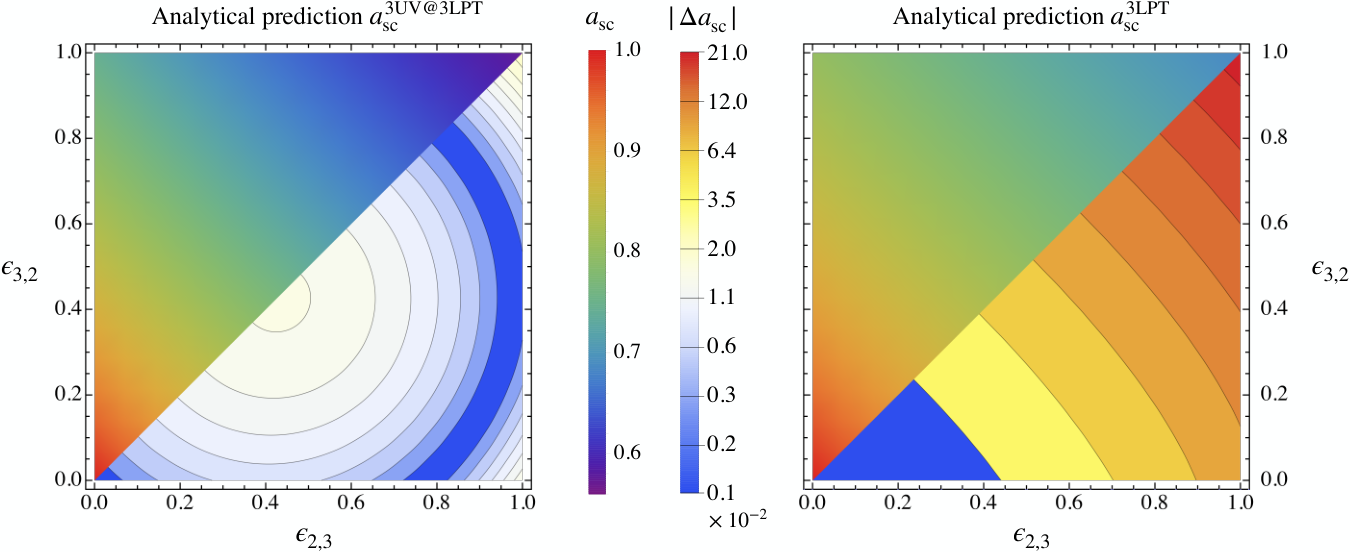
Using this argument, it is straightforward to obtain UV formulas that contain exclusively LPT information between orders ; see App. B.3 for details and derivations, where corresponding results are dubbed 3UV@3LPT. In particular, we find the following analytical estimate for the shell-crossing time,
| (51) |
where
| (52) |
In Fig. 11 in the left panel, we show the resulting prediction on the time of shell-crossing as a function of the initial amplitudes (top-left triangle), and compare it against the one obtained from the nonlinear fitting method (bottom-right triangle; based on Eq. 13). Except for highly symmetric cases where , the analytical formula (V.5) can reproduce the fully nonlinear estimate to an accuracy of better than 1.6%. The quality of this prediction should be compared against the one solely based on standard 3LPT, which we show in the right panel of Fig. 11: here the errors can go up to 21.2% for . Thus, by exploiting the UV method at just third order, we are able to retrieve shell-crossing estimates that are up to an order of magnitude more accurate as compared to 3LPT. We remark that this poor performance of LPT gets alleviated at larger orders, however only slowly: For example, the 10LPT-predictions for the shell-crossing time have errors of up to 5.3%; see App. B.3 and in particular Fig. 24 for further results. Thus, formula (V.5) comes with a performance that is even better than 10LPT.
VI Tidal effects
Here we investigate perturbative solutions for collapsing structures in the presence of an external tidal field, where the latter is assumed to be induced by a long-wavelength perturbation (in the density, gravitational potential, etc.). Similar avenues have been performed in the literature, albeit their focus is either of numerical nature (e.g. Eisenstein and Loeb 1995; Bond and Myers 1996; Shen et al. 2006; Vogelsberger et al. 2008; Sherwin and Zaldarriaga 2012; Wagner et al. 2015; Reischke et al. 2016; Stücker et al. 2018; Stücker et al. 2021), and/or are related to the biasing problem (e.g. Barreira et al. 2020; Taruya and Akitsu 2021; Voivodic and Barreira 2021). Here, by contrast, we stick to the fluid level and are particularly interested in testing the normal-form reduction in the presence of a simple external tidal field that is constant in space. We leave the extension of the present approach to more sophisticated tidal effects, as well as the development of the UV method with tidal field as future work.
For the present purpose, it is sufficient to limit ourselves to the following initial gravitational potential,
| (53) |
where is given in Eq. (7) which acts as the ’short-mode’ input, while is an external tidal field tensor that is symmetric and, as a special requirement, without any contributions in the diagonal components. We note that the last requirement could be easily rectified if needed, but we ignore it here as its main purpose is to readjust the amplitudes of the short-mode input. Furthermore, we assume that is a small quantity w.r.t. to the short-mode input (i.e., for any ); consequently, we only keep displacement terms that are linear in (which in the present case implies quadratic contributions in to ; see discussion below). In summary, we take the tidal-field tensor to be of the form
| (54) |
where are sufficiently small parameters.
In the following section, we determine standard LPT solutions based on . Normal-form reductions are investigated in Sec. VI.2 and discussed in Sec. VI.3.
VI.1 Standard LPT solutions
Using (53) as the input in the recursive relations (6) upon the replacement , it is straightforward to determine the resulting LPT displacements. Keeping only linear terms in , they read
| (55a) | ||||
| (55b) | ||||
and so on, where here and below we attach a “tot” to all fields and solutions that are based on the initial data (53). For the present purpose we determined solutions with tidal field up to order 6LPT.
It is interesting to compare the results (55) with those obtained without external tidal field (section II.2): While the first-order displacements differ, the second-order displacements do actually coincide (cf. eqs. 8 with eqs. 55; this agreement is lost when keeping nonlinear terms in ). Beyond second order, however, the displacements based on (7) and (53) are in general distinct (except some of its gradients; see below).
Due to the presence of an external tidal field, the Jacobian matrix is not diagonal at shell-crossing location; it reads
| (56) |
at order 3LPT, where the displacement terms are evaluated at . Furthermore, we have defined ()
| (57) |
where, from here on, underlined and repeated indices are fixed and thus not summed over; furthermore, we have and the notation means to sort the components in size before evaluating the interior of the square bracket.
The Jacobian matrix (56) has several interesting properties that are worthwhile to emphasize: first, the gradients in (56) can be determined from the initial data with or without linear tidal field (54); that is, we have the identity that, for any
| (58) |
which we have explicitly verified up to order 6LPT (this identity would trivially be falsified if the external tidal field tensor had also non-zero entries on its diagonal). Second, the off-diagonal elements of (56) are nonzero and evolve in time at shell-crossing location, which is in stark contrast to the case without external tidal field. Furthermore, these off-diagonal terms are exactly linear in , and this at any order in LPT, essentially by construction as we keep only linear terms in . This however also implies that the off-diagonal elements contribute to the Jacobian determinant, , despite the fact that these contributions in are actually quadratic in . We choose to keep these nonlinear terms in , as they affect the density and, of course, also the eigenvalues of ; the latter is a consequence that matrix diagonalization is inherently a nonlinear operation (see Ref. Feldbrugge et al. 2023 for related arguments in a somewhat similar context).
In the following section we apply the normal-form reduction to the above collapse case with tidal field; see Sec. VI.3 for the discussion of the LPT and LPT-N results.
VI.2 Linear tidal fields and normal-form reduction
Instead of using the sine-wave initial data (53) with external tidal field, we employ here its normal-form reduction
| (59) |
and test the resulting perturbative predictions, where is given in Eq. (54). To do so we choose the second-order normalization condition (Eq. 30) for which the normal-form displacement is given by ()
| (60) |
where is determined by Eq. (6a) upon the replacement . The resulting displacement coefficients are
| (61) | ||||
| (62) |
and the Jacobian matrix is
| (63) |
at order 3LPT, where can be read off from Eq. (41) and thus, similarly as in the previous section, we have here the identity . The normal-form matrix (63) coincides exactly with (56) to order 2LPT, which is here since we assume vanishing contributions in the diagonal components of . Beyond second order, however, there are differences: The normal-form result has only off-diagonal entries at first order but not beyond, basically by construction. Specifically, the normalization condition (30) sets to zero all off-diagonal entries of beyond first order, which is, of course, in the present case an unwanted feature. Evidently, the normalization condition should be updated in order to accommodate for the evolution of the off-diagonal components in the presence of external tidal fields. However, despite the described shortcoming, we find that the normalization condition (30) comes already with a surprisingly good performance. Therefore we stick with this condition and leave a more accurate modeling with tidal fields for future work.
We remark that a similar negligence of off-diagonal evolution in the Jacobian matrix appears also in so-called triaxial collapse models (e.g. Shen et al. 2006; Vogelsberger et al. 2008; Stücker et al. 2018), where one follows numerically the evolution of an initially diagonalized Jacobian matrix (i.e., its eigenvalues). However, as we have just seen above (see specifically eq. 56), this diagonal feature of the Jacobian matrix is lost during the gravitational evolution, essentially because of nonlinear couplings between short-mode (local) physics with (linear) external tidal fields, which appear to be not encapsulated in such triaxial collapse models.
VI.3 Results with tidal fields
As discussed above, the Jacobian matrix is in general not in diagonal form at shell-crossing location, especially not in the presence of external tidal fields. Depending on the task at hand, it might be beneficial to diagonalize , which is however only possible for fixed Lagrangian location as well as for fixed time. In other words, one may diagonalize at given (initial) time, but the subsequent nonlinear evolution will generally re-populate the off-diagonal components of . Of course, this re-population can be stalled by re-diagonalizing the time-evolved .
Figure 12 shows the temporal evolution of the three (rescaled) eigenvalues that we obtained from the continuous-in-time diagonalization of . All shown solutions are truncated at sixth order in perturbation theory, and the top panel displays in solid [dotted] line style the 6LPT solution with [without] tidal fields based on eq. (56), where we set , and []. In the bottom panel of Fig. 12, we show ratios of from the normal-form considerations versus the LPT predictions, both evaluated at truncation order six. It is seen that the normal-form solutions agree reasonably well with the LPT predictions, despite the fact that nonlinear couplings in the off-diagonal components of are muted in the normal-form case with the second-order normalization condition (cf. discussion in the previous section but also further below for further comments).
Despite the specific choices of tidal parameters made for Fig. 12, we have observed the following general trends for a variety of settings for the components of (we also tested sign flips): The primary axis () always collapses faster in the presence of a linear tidal field, while collapse along the tertiary axis () is always delayed. By contrast, there is no conclusive trend as regards to the secondary axis in the presence of tidal fields, as such a question appears to be decided by subtleties in the initial conditions.
The top panel of Fig. 13 shows predictions for the shell-crossing time at fixed order in LPT (various colors) as a function of a ’tidal stretching parameter’ —for three settings of initial amplitudes (as indicated by various line styles). Generally, for fixed initial amplitudes but large [small] stretching parameter , we observe a smaller [larger] spread in the prediction of for varying truncation orders . This behavior is expected, as an increasingly larger external tidal field begins to swamp the local collapse problem, thereby reducing the relevance of short-mode physics.
In the bottom panel of Fig. 13, we show ratios of the LPT-N versus LPT prediction for varying truncation orders and initial amplitudes. Generally, the normal-form model with second-order normalization condition reproduces the fixed-order LPT results to an accuracy of better than %, which is somewhat surprising considering that this normalization ignores the nonlinear evolution of the off-diagonal components of the Jacobian matrix. It would be interesting to perform the above analysis beyond sixth order in LPT, in particular to be able to analyze whether the normal-form technique leads to a further improvement deep in the UV regime (or, if the gauge conditions should be revisited). Unfortunately, such tasks go beyond the scope of the present study, as, at this stage, we only have access to 6LPT with tidal field—which is also insufficient for performing a detailed analysis of the UV method with tidal field. We will come back to such avenues in future work, where we also allow for a spatially varying external tidal field.
VII Summary and concluding remarks
Summary. Lagrangian perturbation theory accurately predicts the evolution of collisionless matter until the instance of shell-crossing—the crossing of particle trajectories. By doing so, LPT is able to resolve the formation process of primordial dark-matter halos with extreme matter densities, which is a striking success over its perturbative counterpart in Eulerian coordinates. However, except for collapse that occurs largely along a single coordinate axis Rampf and Frisch 2017; Saga et al. 2018, convergence of the LPT series is slow which severely hampers the range of applications. Even worse, the LPT series diverges in voids after some critical time (e.g. Munshi et al. 1994; Sahni and Shandarin 1996; Nadkarni-Ghosh and Chernoff 2011), although physically nothing ’special/extreme’ is happening in such regions.
In this article, we have analyzed two independent methods that circumvent some of the shortcomings of standard perturbation theory in various ways. One of the methods implements a UV completion of the LPT series for the tensor of displacement gradients, essentially by adding a remainder to a low-order truncated LPT series solution that encapsulates the critical nature of the gravitational collapse (eq. III.1). Assuming that this tensor has been diagonalized, that remainder has exactly two unknowns per principal axis (cf. discussion in Sec. V.4). These unknowns, the radius of convergence of the LPT series and a critical exponent, can be determined by a simple linear extrapolation technique (Fig. 3).
The UV-completed solution for the triaxial collapse (Fig. 4 and Fig. 7) as well as for the nonlinear density (Figs. 8–10) compare favorably with independent results—the latter are either obtained through a computationally demanding nonlinear fitting method leading to extrapolation results at order infinity (see Sec. II.2), or from exploiting newly established correspondences to spherical and cylindrical collapse (see further below for details). We remark that the involved extrapolation technique in the UV method formally requires LPT solutions at large orders, in the present case retrieved from 10LPT, but we have also tested a simplified extrapolation method with only 3LPT input that comes with explicit formula for the time of shell-crossing (Sec. V.5), as well as with an excellent performance especially in void regions (see also App. B.3).
The second considered method exploits normal-form techniques, which involve physically motivated, truncated Taylor expansions about a critical point in space. In the present case it is the initial gravitational potential that is Taylor expanded up to second order about the shell-crossing location. The LPT recursive relations (6) still apply in this case, but the displacement field is not anymore constructed from a standard Helmholtz decomposition, essentially since the involved divergence and curl parts of the displacement are just locally evaluated. Instead, we introduce an adapted Helmholtz decomposition for the normal-form displacement field (eq. 29), which comes with an auxiliary vector field that requires a normalization condition. For the latter we demand that the normal-form Jacobian matrix matches the Jacobian matrix at shell-crossing location to second order in standard LPT (eq. 30), which comes with an overall excellent performance. With this second-order normalization condition, the normal-form displacement is determined up to 10th order in perturbation theory in a fraction of a second—on contemporary laptops in single-core mode—instead of a day in standard LPT.
The normal-form solutions reproduce the one from standard LPT to high accuracy; for example, the respective predictions of the shell-crossing time at fixed order—as well as at order infinity—agree at the sub-percent level (Fig. 6). Similar accuracy levels are achieved with the normal-form method when predicting the triaxial evolution and the nonlinear density, even in the presence of a linear external tidal field (Sec. VI and in particular Fig. 12), provided one limits the analysis to the regime of LPT convergence. In voids at times well beyond LPT convergence, the normal-form LPT series is flawed for the same reasons as the LPT one, but this can be easily rectified by pursuing the UV completion applied to the normal-form approach (Sec. IV.1): Indeed, the UV-completed normal-form results (faint lines in e.g. Figs. 7–9) exemplify a similar good performance as their LPT-UV counterparts.
For the case of exactly symmetric sine-wave collapse in 3D (, dubbed S3D), the normal-form predictions actually coincide with those from LPT at shell-crossing location.
A detailed analysis of this specific collapse case reveals a newly established correspondence between S3D and spherical collapse (Sec. IV.3).
For the latter there exists a parametric solution Tolman 1934; Peebles 1967, which thus can be exploited to retrieve a nontrivial prediction for symmetric sine-wave collapse (black dashed lines in Fig. 4 and Fig. 10). We remark that a similar correspondence persists also for the two-dimensional version of the symmetric-sine-wave collapse and cylindrical collapse, albeit for the latter we are not aware of an exact analytical solution; nonetheless we can exploit this correspondence to determine the time of shell-crossing to an accuracy of at least five significant digits; see App. A for details.
Concluding remarks. We have exploited two complementary aspects of criticality in the context of gravitational collapse. One of them is related to the evolutive character of the collapse in the sense of a classical phase transition, which in Lagrangian coordinates is realized by adding a critical term to the displacement, where is the critical exponent. The other critical aspect relates to the spatial character of the collapse, which is encapsulated by a normal-form theory developed at the critical location of the first shell-crossing.
Although we have focused on a restricted class of initial conditions, we believe that our findings display quite generic features of the gravitational collapse. Indeed, three sine waves—or even more its normal form, are largely representative of high peaks of Gaussian random fields (e.g. Bardeen et al. 1986), which is thus relevant for cosmological structure formation.
One obvious next step is to apply the UV and normal-form methods to the gravitational collapse for random-field initial conditions. For the UV method, there is already numerical evidence that the asymptotic behavior for the displacement gradients are all encapsulated by critical terms as outlined above (see also Sec. V.4), although the effects of UV cutoffs on the initial power spectra remain to be investigated Rampf and Hahn 2021; Schmidt 2021.
Regarding the normal-form method, further research is required especially to investigate the impact of nonlocal tidal effects. Indeed, even with the simplified tidal-field model as employed in the present article (e.g., no assumed spatial dependence), the currently employed normalization condition ignores the nonlinear evolution of the off-diagonal elements of the Jacobian matrix (or deformation tensor). While the consequences for the present considerations are fairly marginal (see bottom panel of Fig. 12), the situation is likely to change for more realistic tidal fields.
The UV and normal-form methods could be applied to determine the one-point probability distribution function of the nonlinear matter density for generic (i.e., non-spherical) collapse cases, for example applied in (variants of) excursion set theory; see e.g. Refs. Sheth 1998; Scherrer and Gaztañaga 2001; Lam and Sheth 2008; Klypin et al. 2018; Desjacques et al. 2018; Rampf and Hahn 2023 for possible starting points. Generally, the UV and normal-form methods could be used in a vast range of hybrid approaches where its predictions are paired with a numerical (or another theoretical) technique.
Lastly, in this article we did not consider post-shell-crossing effects which, for generic initial conditions, comprises still a major challenge. From the theory side, this is currently attacked from two vastly different views. The first class of approaches are rather agnostic ones, where some field-level statistics (e.g., the matter power spectrum) are obtained by exploiting renormalization techniques or effective approaches that do not attempt to follow the post-shell-crossing evolution on the deterministic level (e.g. Valageas 2004; Crocce and Scoccimarro 2006; McDonald 2007; Matarrese and Pietroni 2007; Matarrese and Pietroni 2008; Pietroni 2008; Matsubara 2008; Carrasco et al. 2012; Carlson et al. 2013; Blas et al. 2013; Bartelmann et al. 2019). The second class of approaches are the deterministic ones which so far, however, are only worked out for one-dimensional collapse Colombi 2015; Taruya and Colombi 2017; Rampf and Frisch 2017; see however Ref. Saga et al. 2022 for first steps in 3D exploiting ballistic approximations. We expect that the presently discussed UV and normal-form methods could first generate some impact for the second class of approaches. Nevertheless, it would be interesting to investigate whether the methods could also improve the theoretical modeling within effective fluid descriptions or similar approaches, thereby also assisting to reduce the gap between the various approaches in theoretical and numerical structure formation.
Acknowledgements.
C.R. thanks Oliver Hahn for useful discussions. This work was supported by JSPS Overseas Research Fellowships (S.S.) and in part by MEXT/JSPS KAKENHI Grant Numbers JP20H05861, JP21H01081, and JST AIP Acceleration Research Grant Number JP20317829 (A.T.), as well as Programme National Cosmology et Galaxies (PNCG) of CNRS/INSU with INP and IN2P3, cofunded by CEA and CNES (S.C.).Appendix A Analysis for two-dimensional collapse
By now, LPT recursive relations in 3D are fairly well exploited Rampf 2012; Zheligovsky and Frisch 2014; Rampf et al. 2015; Matsubara 2015; Rampf et al. 2022, but this is not so for the 2D case; therefore this case is reviewed in the following (see also Saga et al. 2022). Afterwards, in Sec. A.2, we establish a correspondence between the symmetric sine-wave model in 2D and cylindrical collapse, which we exploited in Sec. IV.3 to retrieve a highly accurate prediction of the shell-crossing time for S2D (see e.g. Table 1). Finally, at the end of Sec. A.2, we provide a physical analysis for cylindrical collapse/S2D.
A.1 Evolution equations and LPT recursive relations in 2D
Suppose that the initial data depends only on two of the three space coordinates. Then, the gravitational evolution of this fluid system is still governed by the standard three-dimensional equations in Lagrangian coordinates. However, due to this embedding of a two-dimensional problem in 3D space, all space derivatives in the “third” dimension (say in direction) vanish trivially. As a consequence, the Lagrangian evolution equations simplify and read in an EdS universe Saga et al. 2022
| (64) |
where is the two-dimensional antisymmetric tensor, summation over repeated indices is assumed but now excludes if not otherwise stated, , and the Jacobian determinant is now . The second of the equations in (64) are the Cauchy invariants formulated in 2D which, to our knowledge, have first been investigated in Ref. Podvigina et al. 2016 however in a non-cosmological context.
Equations (64) can also be written for the 2D displacement,
| (65) | ||||
| (66) |
which can be easily solved by the usual Ansatz , leading to the all-order recursive relations
| (67a) | ||||
| where , and . Likewise, for the (pseudo-) vector part we have the only non-zero contribution in the direction: | ||||
| (67b) | ||||
| In summary the 2D displacement coefficient at th order is | ||||
| (67c) | ||||
As a simple example, let us determine the first few displacement coefficients for the case of symmetric sine-wave collapse in 2D, for which we take the initial data to be
| (68) |
Using this as the input in the recursive relations (67), one straightforwardly finds the 2D displacement coefficients
| (69) | ||||
| (70) |
and so on. The corresponding Jacobian matrix is diagonal at shell-crossing location , and has the determinant
| (71) |
up to fourth order in perturbation theory. In the following we compare this result against complementary derivations based on cylindrical collapse, which reveals the anticipated correspondence between cylindrical collapse and S2D.
A.2 Cylindrical collapse and correspondence to S2D
Here we consider the so-called cylindrical collapse, which we define as a ’top-hat’ perturbation in 2D (i.e., analogously to the spherical collapse in 3D). To our knowledge, there exists no exact analytical solution for cylindrical collapse.
To make progress on the problem, one may employ cylindrical coordinates. Likewise, however, this task can also be tackled in a Cartesian setup for which the Jacobian matrix must be exactly diagonal with identical entries (see e.g. Hui and Bertschinger 1996; Mukhanov 2005; Rampf 2019; Rampf and Hahn 2023 for similar considerations, also applied to the spherical case). Within such a setup, we can apply normal-form arguments as outlined in this work to provide appropriate initial conditions of the form
| (72) |
where is an a priori arbitrary curvature scale. Furthermore, we employ the so-called slaving boundary conditions on the initial conditions, which adjusts a specific relationship between the velocity and the gravitational potential at initial time , thereby effectively setting decaying modes to zero (see e.g. Brenier et al. 2003b; Rampf 2019 for details). Finally, due to the perfect 2D symmetry, we can impose a refined Ansatz for the Jacobian matrix
| (73) |
where are time- and space-independent Taylor coefficients that we determine in the following. For this one could employ the recursive relations (67) but, thanks to this refined Ansatz, we can actually do much better: plugging (73) into the Lagrangian evolution equations (64) and identifying the involved powers in , we find the vastly simplified recursive relations ()
| (74) |
The first few contributions are
| (75) |
but higher-order contributions are very swiftly determined by employing standard linear algebra programs. For the purpose of this work we determined analytically the coefficients up to order , which takes about three hours on a contemporary laptop in single-core mode (determining the first 1000 coefficients are a matter of seconds).
Correspondence between cylindrical collapse and S2D. Calculating the Jacobian determinant based on the above solutions reveals straightforwardly
| (76) |
up to fourth order in perturbation theory. Evidently, for the choice , this result agrees exactly with the one obtained for S2D as reported in Eq. (71), thereby establishing immediately the anticipated correspondence. We have explicitly verified this correspondence up to LPT order .
Asymptotic results. Before investigating the physical regime of validity of the cylindrical displacement, let us determine the leading-order asymptotic features of the Taylor series . This can be done by drawing the Domb–Sykes plot, which we have motivated around Eq. (18) in the main text. Figure 14 shows the corresponding ratios of subsequent Taylor coefficients versus (orange dots), as well as a linear regression (black dashed line) which is the result from a linear interpolation between LPT orders (using instead or any other choice within this interval has at most a effect on the fitting parameters). Extrapolating this linear regression to the -intercept reveals that the cylindrical displacement behaves at very large Taylor orders as
| (77) | ||||
| where | ||||
| (78) | ||||
Thus, based on these asymptotic results, we theoretically predict a blowup of the second time derivative of the cylindrical displacement (i.e., the particle acceleration) at . We have explicitly verified this statement by employing the nonlinear extrapolation method of Ref. Saga et al. 2018, which also predicts a spiky feature at shell-crossing location when drawing the acceleration over the current position.
Physical analysis of cylindrical collapse/S2D. The above established correspondence allows us to perform swiftly a physical analysis for S2D collapse at extremely high perturbation orders. One obvious task is then to determine the time of first shell-crossing, which in the present case reduces to the root-finding problem
| (79) |
where . However, at increasingly large perturbation orders (), the numerical root finding algorithm is quickly limited by numerical precision, basically since the employed computer algebra program is summing up a large number of numerically small terms. We circumvent this problem by exploiting the following property: for this notice that the Taylor series of the cylindrical displacement is comprised of only rational Taylor coefficients and thus, the obvious source of numerical errors stems from multiplying these rational coefficients by numerical values of . Therefore, before numerically evaluating , we rationalize the numerical values of for increasingly higher precision, which allows us to determine for large essentially to machine precision. Our most accurate result is obtained at order for which the shell-crossing time is ()
| (80) |
Observe that this shell-crossing estimate agrees with the above reported to a precision of five significant digits, which strongly suggests that . This result is not completely surprising as we know that a similar congruence exists also for spherical collapse Rampf and Hahn 2023.

In Fig. 15 we show the temporal evolution of the physical trajectory for various truncation orders . Specifically, to not clutter the figure we show results for LPT orders (solid lines, from blue to red) as well as the 1000LPT result (black dashed line). Similarly as observed in the spherical case, LPT convergence for cylindrical collapse is fairly slow—which however could be vastly accelerated by the UV method. Indeed, for 5UV using just 10LPT as the extrapolation input, we find (see Table 1), which agrees against the (supposedly) exact result (78) to a precision of about %.
Finally, in Fig. 16 we show various theoretical predictions for the nonlinear density contrast, based on S2D (various colors) and for cylindrical collapse (black dashed line). As expected, 1000LPT and 5UV agree to high precision within the range of LPT convergence (gray shaded area). Beyond convergence which is in particular relevant for very low densities, however, the UV and UV-N predictions become substantially more reliable which is also expected.
For completeness we have also added in Fig. 16 our prediction for the linear density at collapse time (vertical gray-dashed line), .
Appendix B More results for the UV method
Here we provide more results to the UV method. Specifically, asymptotic results are discussed in the following section, while we provide further results to triaxial collapse in Sec. B.2. Finally, in Sec. B.3 we introduce a vastly simplified implementation of the UV method in explicit form, which only requires 3LPT input.
B.1 Asymptotic results in transverse directions
The UV method requires some knowledge of the asymptotic behavior of the LPT displacement series (see Sec. III.1). In the main text we focused on the asymptotic analysis of the gradient along the primary axis of the displacement coefficients, i.e., ; this analysis led to the Domb–Sykes figure and results for the unknowns in the UV method as given in Fig. 3. Here we show the asymptotic results for the ’transverse’ gradients, and , which are e.g. needed in the UV method when predicting the temporal evolution of all three eigenvalues of the Jacobian matrix (Fig. 7) and the nonlinear density (Figs. 8–10).
In Fig. 17 we show the Domb–Sykes plots for the transverse displacement gradients at shell-crossing location, specifically for in the top panel and in the lower panel, based on the initial data (7). In the 3D axisymmetric case (S3D; black dots) the Domb–Sykes results of course coincide for all three gradients, but in general the resulting values for and retrieved from the asymptotic analysis are different (see Sec. III.1 for details of the procedure). In the same figures we also show the results for the normal-form method (faint lines), where the asymptotic results for and coincide exactly with ; this congruence has been addressed in the final paragraph of Sec. IV.4 for which we kindly refer the readers for details.
B.2 Triaxial evolution
Here we show further results related to the temporal evolution of the three eigenvalues of the Jacobian matrix, based on the tidal-field-free model with initial data (7). Specifically, in the top panel of Fig. 18 we show the triaxial evolution of (various line styles) for three choices of initial amplitudes (various colors). For S3D which assumes (black), the temporal evolution of all three ’s is identical and, as expected, the UV-N prediction overlaps exactly with the UV prediction (cf. Fig. 4 and related discussion).
Here we remark again that none of the shown results can be trusted once the first axis collapses, which can also be seen in Fig. 19 where faint lines denote LPT results. As soon as LPT convergence is lost (indicated by the shadings), which is at, or shortly after, the first shell-crossing, the Jacobian becomes unphysically large which indicates that the large-density region dissolves again—this is a known and well documented problem of standard perturbation theory; see e.g. Ref. Rampf 2021 and references therein.
B.3 Fast asymptotic predictions for the UV method at 3LPT
One of the key aspect of the UV [and UV-N] method is that some knowledge of the asymptotic knowledge of the LPT [LPT-N] series is required in order to perform the completion to order infinity. As argued in Sec. III.1, this knowledge can be retrieved by considering ratios of LPT displacement gradients (cf. Eq. 18)
| (81) |
where repeated and underlined indices are not summed over, while and are the unknowns of the asymptotic extrapolation with gradient component (the above trivially generalizes to off-diagonal components in if nonzero). Note specifically that, as opposed in the main text, we now keep the component dependencies of and explicit.
The UV and UV-N results presented in the main text employ for the asymptotic extrapolation as input the LPT [LPT-N] results between orders . Here we test the accuracy of the predictions if instead the extrapolation is performed at the orders . Actually the 3LPT [3LPT-N] input is the absolute minimum for the asymptotic considerations as one gets exactly two data points, namely from the ratios and (i.e., the first two data points from the right in Fig. 17). In this case a fitting procedure is of course not needed as the two data tuples are exactly connected by a linear regression. These considerations lead straightforwardly to the explicit results for the unknowns and . For the LPT model we find, for
| (82a) | ||||
| (82b) | ||||
| for | ||||
| (82c) | ||||
| (82d) | ||||
| and for | ||||
| (82e) | ||||
| (82f) | ||||
The above is also straightforwardly generalized to the off-diagonal components of the displacement gradient which is generally needed when the Jacobian matrix is not in diagonal form. Furthermore, the same arguments also apply to the normal-form case, from which one retrieves explicit expressions for and (not shown).
The explicit expressions for and can be directly used in the 3UV description for the three displacement gradients, which are respectively
| (83) |
| (84) |
| (85) |
thereby leading to an analytical prediction of the eigenvalues of the Jacobian matrix
| (86) |
as well as for the nonlinear density contrast
| (87) |
at shell-crossing location. If required (e.g. for Press–Schechter formalism), the latter can also be recast so that the nonlinear density is a function of the linear density contrast . Thus, with the above results one obtains a complete description that, as promised, is solely based on 3LPT [3LPT-N] considerations; above and in the following we call the respective prediction 3UV@3LPT [3UV-N@3LPT-N]. Similarly, 3UV and 3UV-N predictions with 10LPT input are dubbed 3UV@10LPT and 3UV-N@10LPT-N, respectively.
Figure 20 shows in green the resulting predictions for the evolution of the first eigenvalue of the Jacobian matrix with 3UV@3LPT [faint green line: 3UV-N@3LPT-N] for the exactly symmetric sine-wave collapse. For comparison we have added also the UV predictions from the main text which take 10LPT as extrapolation input. By direct comparison with the parametric result (black dotted line), it is evident that 3UV@3LPT is extremely accurate, especially in void regions where it even outperforms 3UV@10LPT (magenta dashed line). In Fig. 21 we show for an asymmetric collapse with and . While we do not have an exact solution at hand, also here 3UV@3LPT and its normal form appear to exemplify a convincing performance overall.
A similarly good performance for 3UV@3LPT is observed for predicting the nonlinear density contrast, shown in Fig. 22 for the S3D case (see also Fig. 23 for the asymmetric case). Note that, in comparison with the complementary Figs. 8 and 10, we greatly expanded the void regime in these density plots, while the agreement between the UV prediction with 3LPT input and the theoretical prediction is still sub-percent.
Finally, the above considerations can also be used to retrieve an accurate formula for the time of first shell-crossing. Specifically, assuming the ordering for which shell-crossing occurs along the first diagonal component in the Jacobian matrix, we impose , which yields

| (88) |
where
| (89) |
Again, all these derivations are exact and have been carried out with only information up to 3LPT.
In Fig. 24 we compare the just obtained analytical formula for the shell-crossing time (cyan line) versus LPT (Eq. 10, various colors), as well as against the estimate at order infinity based on the nonlinear fitting procedure from the main text (Eq. 13, black dotted line). It is seen that the purely analytical 3UV@3LPT prediction agrees against the nonlinear extrapolation result to better than 2% for all considered initial amplitudes (see also Fig. 11 in the main text). This performance should also be compared against fixed-order LPT in particular 3LPT (right panel in Fig. 11 and Fig. 24): evidently, 3LPT performs much worse than 3UV@3LPT with errors reaching 21.2% for —despite the fact that the theoretical input of both methods is identical.
References
- P. A. Abell et al. (2009) (LSST Science Collaboration) P. A. Abell et al. (LSST Science Collaboration), (2009), arXiv:0912.0201 [astro-ph.IM] .
- R. Laureijs et al. (2011) (Euclid collaboration) R. Laureijs et al. (Euclid collaboration), (2011), arXiv:1110.3193 [astro-ph.CO] .
- H. Aihara et al. (2018) (HSC collaboration) H. Aihara et al. (HSC collaboration), Publ. Astron. Soc. Jap. 70, S8 (2018), arXiv:1702.08449 [astro-ph.IM] .
- A. Weltman et al. (2020) (SKA collaboration) A. Weltman et al. (SKA collaboration), Publ. Astron. Soc. Aust. 37, e002 (2020), arXiv:1810.02680 [astro-ph.CO] .
- Peebles (1980) P. J. E. Peebles, The large-scale structure of the universe (Princeton University Press, Princeton, NJ, 1980).
- Fry (1984) J. N. Fry, Astrophys. J. 279, 499 (1984).
- Bernardeau et al. (2002) F. Bernardeau, S. Colombi, E. Gaztañaga, and R. Scoccimarro, Phys. Rep. 367, 1 (2002), arXiv:astro-ph/0112551 .
- Jasche and Wandelt (2013) J. Jasche and B. D. Wandelt, Mon. Not. Roy. Astron. Soc. 432, 894 (2013), arXiv:1203.3639 [astro-ph.CO] .
- Kitaura (2013) F. S. Kitaura, Mon. Not. Roy. Astron. Soc. 429, L84 (2013), arXiv:1203.4184 [astro-ph.CO] .
- Wang et al. (2013) H. Wang, H. J. Mo, X. Yang, and F. C. van den Bosch, Astrophys. J. 772, 63 (2013), arXiv:1301.1348 [astro-ph.CO] .
- Ata et al. (2021) M. Ata, F.-S. Kitaura, K.-G. Lee, B. C. Lemaux, D. Kashino, O. Cucciati, M. Hernández-Sánchez, and O. Le Fèvre, Mon. Not. Roy. Astron. Soc. 500, 3194 (2021), arXiv:2004.11027 [astro-ph.CO] .
- Kitaura et al. (2012) F.-S. Kitaura, S. Gallerani, and A. Ferrara, Mon. Not. Roy. Astron. Soc. 420, 61 (2012), arXiv:1011.6233 [astro-ph.CO] .
- Metcalf et al. (2018) R. B. Metcalf, R. A. C. Croft, and A. Romeo, Mon. Not. Roy. Astron. Soc. 477, 2841 (2018), arXiv:1706.08939 [astro-ph.CO] .
- Porqueres et al. (2020) N. Porqueres, O. Hahn, J. Jasche, and G. Lavaux, Astron. Astrophys. 642, A139 (2020), arXiv:2005.12928 [astro-ph.CO] .
- Ravoux et al. (2020) C. Ravoux, E. Armengaud, M. Walther, T. Etourneau, D. Pomarède, N. Palanque-Delabrouille, C. Yèche, J. Bautista, H. du Mas des Bourboux, S. Chabanier, K. Dawson, J. M. Le Goff, B. Lyke, A. D. Myers, P. Petitjean, M. M. Pieri, J. Rich, G. Rossi, and D. P. Schneider, J. Cosmol. Astropart. Phys. 2020, 010 (2020), arXiv:2004.01448 [astro-ph.CO] .
- Klypin and Shandarin (1983) A. A. Klypin and S. F. Shandarin, Mon. Not. Roy. Astron. Soc. 204, 891 (1983).
- Efstathiou et al. (1985) G. Efstathiou, M. Davis, S. D. M. White, and C. S. Frenk, Astrophys. J. Suppl. 57, 241 (1985).
- Scoccimarro (1998) R. Scoccimarro, Mon. Not. Roy. Astron. Soc. 299, 1097 (1998), arXiv:astro-ph/9711187 [astro-ph] .
- Crocce et al. (2006) M. Crocce, S. Pueblas, and R. Scoccimarro, Mon. Not. Roy. Astron. Soc. 373, 369 (2006), arXiv:astro-ph/0606505 [astro-ph] .
- Michaux et al. (2021) M. Michaux, O. Hahn, C. Rampf, and R. E. Angulo, Mon. Not. Roy. Astron. Soc. 500, 663 (2021), arXiv:2008.09588 [astro-ph.CO] .
- Tassev et al. (2013) S. Tassev, M. Zaldarriaga, and D. J. Eisenstein, J. Cosmol. Astropart. Phys. 2013, 036 (2013), arXiv:1301.0322 [astro-ph.CO] .
- Howlett et al. (2015) C. Howlett, M. Manera, and W. J. Percival, Astron. Comput. 12, 109 (2015), arXiv:1506.03737 [astro-ph.CO] .
- Feng et al. (2016) Y. Feng, M.-Y. Chu, U. Seljak, and P. McDonald, Mon. Not. Roy. Astron. Soc. 463, 2273 (2016), arXiv:1603.00476 [astro-ph.CO] .
- Chartier et al. (2021) N. Chartier, B. Wandelt, Y. Akrami, and F. Villaescusa-Navarro, Mon. Not. Roy. Astron. Soc. 503, 1897 (2021), arXiv:2009.08970 [astro-ph.CO] .
- Kokron et al. (2021) N. Kokron, J. DeRose, S.-F. Chen, M. White, and R. H. Wechsler, Mon. Not. Roy. Astron. Soc. 505, 1422 (2021), arXiv:2101.11014 [astro-ph.CO] .
- Zennaro et al. (2023) M. Zennaro, R. E. Angulo, M. Pellejero-Ibáñez, J. Stücker, S. Contreras, and G. Aricò, Mon. Not. Roy. Astron. Soc. 524, 2407 (2023), arXiv:2101.12187 [astro-ph.CO] .
- Aricò et al. (2022) G. Aricò, R. E. Angulo, and M. Zennaro, Open Research Europe 1, (2022), arXiv:2104.14568 [astro-ph.CO] .
- Buchert and Götz (1987) T. Buchert and G. Götz, J. Math. Phys. 28, 2714 (1987).
- Buchert (1989) T. Buchert, Astron. Astrophys. 223, 9 (1989).
- Moutarde et al. (1991) F. Moutarde, J. M. Alimi, F. R. Bouchet, R. Pellat, and A. Ramani, Astrophys. J. 382, 377 (1991).
- Buchert (1994) T. Buchert, Mon. Not. Roy. Astron. Soc. 267, 811 (1994), arXiv:astro-ph/9309055 [astro-ph] .
- Bouchet et al. (1995) F. R. Bouchet, S. Colombi, E. Hivon, and R. Juszkiewicz, Astron. Astrophys. 296, 575 (1995), arXiv:astro-ph/9406013 [astro-ph] .
- Ehlers and Buchert (1997) J. Ehlers and T. Buchert, Gen. Relativ. Gravit. 29, 733 (1997), arXiv:astro-ph/9609036 [astro-ph] .
- Rampf and Frisch (2017) C. Rampf and U. Frisch, Mon. Not. Roy. Astron. Soc. 471, 671 (2017), arXiv:1705.08456 [astro-ph.CO] .
- Saga et al. (2018) S. Saga, A. Taruya, and S. Colombi, Phys. Rev. Lett. 121, 241302 (2018), arXiv:1805.08787 [astro-ph.CO] .
- Rampf and Hahn (2021) C. Rampf and O. Hahn, Mon. Not. Roy. Astron. Soc. 501, L71 (2021), arXiv:2010.12584 [astro-ph.CO] .
- Schmidt (2021) F. Schmidt, J. Cosmol. Astropart. Phys. 2021, 033 (2021), arXiv:2012.09837 [astro-ph.CO] .
- Saga et al. (2022) S. Saga, A. Taruya, and S. Colombi, Astron. Astrophys. 664, A3 (2022), arXiv:2111.08836 [astro-ph.CO] .
- Rampf et al. (2022) C. Rampf, U. Frisch, and O. Hahn, Phys. Rev. Fluids 7, 104610 (2022), arXiv:2207.12416 [physics.flu-dyn] .
- Rampf (2019) C. Rampf, Mon. Not. Roy. Astron. Soc. 484, 5223 (2019), arXiv:1712.01878 [astro-ph.CO] .
- Nadkarni-Ghosh and Chernoff (2011) S. Nadkarni-Ghosh and D. F. Chernoff, Mon. Not. Roy. Astron. Soc. 410, 1454 (2011), arXiv:1005.1217 [astro-ph.CO] .
- Nadkarni-Ghosh and Chernoff (2013) S. Nadkarni-Ghosh and D. F. Chernoff, Mon. Not. Roy. Astron. Soc. 431, 799 (2013), arXiv:1211.5777 [astro-ph.CO] .
- Rampf and Hahn (2023) C. Rampf and O. Hahn, Phys. Rev. D 107, 023515 (2023), arXiv:2211.02053 [astro-ph.CO] .
- Kitaura and Hess (2013) F. S. Kitaura and S. Hess, Mon. Not. Roy. Astron. Soc. 435, L78 (2013), arXiv:1212.3514 [astro-ph.CO] .
- Bernardeau (1994) F. Bernardeau, Astrophys. J. 427, 51 (1994), arXiv:astro-ph/9311066 [astro-ph] .
- Mohayaee et al. (2006) R. Mohayaee, H. Mathis, S. Colombi, and J. Silk, Mon. Not. Roy. Astron. Soc. 365, 939 (2006), arXiv:astro-ph/0501217 [astro-ph] .
- Monaco et al. (2002) P. Monaco, T. Theuns, and G. Taffoni, Mon. Not. Roy. Astron. Soc. 331, 587 (2002), arXiv:astro-ph/0109323 [astro-ph] .
- Monaco et al. (2013) P. Monaco, E. Sefusatti, S. Borgani, M. Crocce, P. Fosalba, R. K. Sheth, and T. Theuns, Mon. Not. Roy. Astron. Soc. 433, 2389 (2013), arXiv:1305.1505 [astro-ph.CO] .
- Stein et al. (2019) G. Stein, M. A. Alvarez, and J. R. Bond, Mon. Not. Roy. Astron. Soc. 483, 2236 (2019), arXiv:1810.07727 [astro-ph.CO] .
- Neyrinck (2016a) M. C. Neyrinck, Mon. Not. Roy. Astron. Soc. 455, L11 (2016a), arXiv:1503.07534 [astro-ph.CO] .
- Tosone et al. (2021) F. Tosone, M. C. Neyrinck, B. R. Granett, L. Guzzo, and N. Vittorio, Mon. Not. Roy. Astron. Soc. 505, 2999 (2021), arXiv:2012.14446 [astro-ph.CO] .
- Monaco (2016) P. Monaco, Galaxies 4, 53 (2016), arXiv:1605.07752 [astro-ph.CO] .
- Lippich et al. (2019) M. Lippich, A. G. Sánchez, M. Colavincenzo, E. Sefusatti, P. Monaco, L. Blot, M. Crocce, M. A. Alvarez, A. Agrawal, S. Avila, A. Balaguera-Antolínez, R. Bond, S. Codis, C. Dalla Vecchia, A. Dorta, P. Fosalba, A. Izard, F.-S. Kitaura, M. Pellejero-Ibanez, G. Stein, M. Vakili, and G. Yepes, Mon. Not. Roy. Astron. Soc. 482, 1786 (2019), arXiv:1806.09477 [astro-ph.CO] .
- Tatekawa (2007) T. Tatekawa, Phys. Rev. D 75, 044028 (2007), arXiv:astro-ph/0605250 [astro-ph] .
- Yoshisato et al. (1998) A. Yoshisato, T. Matsubara, and M. Morikawa, Astrophys. J. 498, 48 (1998), arXiv:astro-ph/9707296 [astro-ph] .
- Matsubara et al. (1998) T. Matsubara, A. Yoshisato, and M. Morikawa, Astrophys. J. 504, 7 (1998), arXiv:astro-ph/9708154 [astro-ph] .
- Taruya et al. (2022) A. Taruya, T. Nishimichi, and D. Jeong, Phys. Rev. D 105, 103507 (2022), arXiv:2109.06734 [astro-ph.CO] .
- Doroshkevich (1970) A. G. Doroshkevich, Astrophysics 6, 320 (1970).
- Moutarde et al. (1995) F. Moutarde, J. M. Alimi, F. R. Bouchet, and R. Pellat, Astrophys. J. 441, 10 (1995).
- Arnol’d (1980) V. I. Arnol’d, Mathematical Methods of Classical Mechanics (Springer, New York, 1980) p. 464.
- Berry and Upstill (1980) M. V. Berry and C. Upstill, Progess in Optics 18, 257 (1980).
- Arnold et al. (1982) V. I. Arnold, S. F. Shandarin, and I. B. Zeldovich, Geophys. Astrophys. Fluid Dyn. 20, 111 (1982).
- DeVille et al. (2008) R. E. L. DeVille, A. Harkin, M. Holzer, K. Josić, and T. J. Kaper, Physica D Nonlinear Phenomena 237, 1029 (2008).
- Hidding et al. (2014) J. Hidding, S. F. Shandarin, and R. van de Weygaert, Mon. Not. Roy. Astron. Soc. 437, 3442 (2014), arXiv:1311.7134 [astro-ph.CO] .
- Feldbrugge et al. (2014) J. L. Feldbrugge, J. Hidding, and R. van de Weygaert, Proc. Int. Astron. 11, 107–114 (2014), arXiv:1412.5121 [astro-ph.CO] .
- Neyrinck (2016b) M. C. Neyrinck, in The Zeldovich Universe: Genesis and Growth of the Cosmic Web, Vol. 308, edited by R. van de Weygaert, S. Shandarin, E. Saar, and J. Einasto (2016) pp. 97–102, arXiv:1412.6114 [astro-ph.CO] .
- Colombi (2015) S. Colombi, Mon. Not. Roy. Astron. Soc. 446, 2902 (2015), arXiv:1411.4165 [astro-ph.CO] .
- Taruya and Colombi (2017) A. Taruya and S. Colombi, Mon. Not. Roy. Astron. Soc. 470, 4858 (2017), arXiv:1701.09088 [astro-ph.CO] .
- Rampf et al. (2021) C. Rampf, U. Frisch, and O. Hahn, Mon. Not. Roy. Astron. Soc. 505, L90 (2021), arXiv:1912.00868 [astro-ph.CO] .
- Brenier et al. (2003a) Y. Brenier, U. Frisch, M. Hénon, G. Loeper, S. Matarrese, R. Mohayaee, and A. Sobolevskiĭ, Mon. Not. Roy. Astron. Soc. 346, 501 (2003a), arXiv:astro-ph/0304214 [astro-ph] .
- Rampf (2012) C. Rampf, J. Cosmol. Astropart. Phys. 2012, 004 (2012), arXiv:1205.5274 [astro-ph.CO] .
- Zheligovsky and Frisch (2014) V. Zheligovsky and U. Frisch, J. Fluid Mech 749, 404 (2014), arXiv:1312.6320 [math.AP] .
- Rampf et al. (2015) C. Rampf, B. Villone, and U. Frisch, Mon. Not. Roy. Astron. Soc. 452, 1421 (2015), arXiv:1504.00032 [astro-ph.CO] .
- Matsubara (2015) T. Matsubara, Phys. Rev. D 92, 023534 (2015), arXiv:1505.01481 [astro-ph.CO] .
- Rampf et al. (2022) C. Rampf, S. O. Schobesberger, and O. Hahn, Mon. Not. Roy. Astron. Soc. 516, 2840 (2022), arXiv:2205.11347 [astro-ph.CO] .
- Sousbie and Colombi (2016) T. Sousbie and S. Colombi, J. Comput. Phys. 321, 644 (2016), arXiv:1509.07720 [physics.comp-ph] .
- Novikov (1969) E. A. Novikov, Sov. Phys. JETP 30, 512 (1969).
- Zentsova and Chernin (1980) A. S. Zentsova and A. D. Chernin, Astrophysics 16, 108 (1980).
- McQuinn and White (2016) M. McQuinn and M. White, J. Cosmol. Astropart. Phys. 2016, 043 (2016), arXiv:1502.07389 [astro-ph.CO] .
- Bardeen et al. (1986) J. M. Bardeen, J. R. Bond, N. Kaiser, and A. S. Szalay, Astrophys. J. 304, 15 (1986).
- Zel’dovich (1970) Ya. B. Zel’dovich, Astron. Astrophys. 5, 84 (1970).
- Rampf and Buchert (2012) C. Rampf and T. Buchert, J. Cosmol. Astropart. Phys. 2012, 021 (2012), arXiv:1203.4260 [astro-ph.CO] .
- Domb and Sykes (1957) C. Domb and M. F. Sykes, Proc. R. Soc. Lond. Series A 240, 214 (1957).
- van Dyke (1974) M. van Dyke, Q. J. Mech. Appl. Math. 27, 423 (1974).
- Magner and Arita (2017) A. G. Magner and K. Arita, Phys. Rev. E 96, 042206 (2017), arXiv:1709.10403 [math.DS] .
- Feldbrugge et al. (2018) J. Feldbrugge, R. van de Weygaert, J. Hidding, and J. Feldbrugge, J. Cosmol. Astropart. Phys. 2018, 027 (2018), arXiv:1703.09598 [astro-ph.CO] .
- Offen and Ober-Blöbaum (2021) C. Offen and S. Ober-Blöbaum, IFAC-PapersOnLine 54, 334 (2021), arXiv:2107.13853 [math.OC] .
- Scherrer and Gaztañaga (2001) R. J. Scherrer and E. Gaztañaga, Mon. Not. Roy. Astron. Soc. 328, 257 (2001), arXiv:astro-ph/0105534 [astro-ph] .
- Pietroni (2018) M. Pietroni, J. Cosmol. Astropart. Phys. 2018, 028 (2018), arXiv:1804.09140 [astro-ph.CO] .
- Rampf (2021) C. Rampf, Rev. Mod. Plasma Phys. 5, 10 (2021).
- Sahni and Shandarin (1996) V. Sahni and S. Shandarin, Mon. Not. Roy. Astron. Soc. 282, 641 (1996), arXiv:astro-ph/9510142 [astro-ph] .
- Munshi et al. (1994) D. Munshi, V. Sahni, and A. A. Starobinsky, Astrophys. J. 436, 517 (1994), arXiv:astro-ph/9402065 [astro-ph] .
- Eisenstein and Loeb (1995) D. J. Eisenstein and A. Loeb, Astrophys. J. 439, 520 (1995), arXiv:astro-ph/9405012 [astro-ph] .
- Bond and Myers (1996) J. R. Bond and S. T. Myers, Astrophys. J. Suppl. 103, 1 (1996).
- Shen et al. (2006) J. Shen, T. Abel, H. J. Mo, and R. K. Sheth, Astrophys. J. 645, 783 (2006), arXiv:astro-ph/0511365 [astro-ph] .
- Vogelsberger et al. (2008) M. Vogelsberger, S. D. M. White, A. Helmi, and V. Springel, Mon. Not. Roy. Astron. Soc. 385, 236 (2008), arXiv:0711.1105 [astro-ph] .
- Sherwin and Zaldarriaga (2012) B. D. Sherwin and M. Zaldarriaga, Phys. Rev. D 85, 103523 (2012), arXiv:1202.3998 [astro-ph.CO] .
- Wagner et al. (2015) C. Wagner, F. Schmidt, C. T. Chiang, and E. Komatsu, Mon. Not. Roy. Astron. Soc. 448, L11 (2015), arXiv:1409.6294 [astro-ph.CO] .
- Reischke et al. (2016) R. Reischke, F. Pace, S. Meyer, and B. M. Schäfer, Mon. Not. Roy. Astron. Soc. 463, 429 (2016), arXiv:1606.09207 [astro-ph.CO] .
- Stücker et al. (2018) J. Stücker, P. Busch, and S. D. M. White, Mon. Not. Roy. Astron. Soc. 477, 3230 (2018), arXiv:1710.09881 [astro-ph.CO] .
- Stücker et al. (2021) J. Stücker, A. S. Schmidt, S. D. M. White, F. Schmidt, and O. Hahn, Mon. Not. Roy. Astron. Soc. 503, 1473 (2021), arXiv:2003.06427 [astro-ph.CO] .
- Barreira et al. (2020) A. Barreira, G. Cabass, F. Schmidt, A. Pillepich, and D. Nelson, J. Cosmol. Astropart. Phys. 2020, 013 (2020), arXiv:2006.09368 [astro-ph.CO] .
- Taruya and Akitsu (2021) A. Taruya and K. Akitsu, J. Cosmol. Astropart. Phys. 2021, 061 (2021), arXiv:2106.04789 [astro-ph.CO] .
- Voivodic and Barreira (2021) R. Voivodic and A. Barreira, J. Cosmol. Astropart. Phys. 2021, 069 (2021), arXiv:2012.04637 [astro-ph.CO] .
- Feldbrugge et al. (2023) J. Feldbrugge, Y. Yan, and R. van de Weygaert, Mon. Not. Roy. Astron. Soc. (2023), 10.1093/mnras/stad2777, arXiv:2301.07200 [astro-ph.CO] .
- Tolman (1934) R. C. Tolman, Relativity, Thermodynamics, and Cosmology (Clarendon Press, Oxford, 1934) p. 528.
- Peebles (1967) P. J. E. Peebles, Astrophys. J. 147, 859 (1967).
- Sheth (1998) R. K. Sheth, Mon. Not. Roy. Astron. Soc. 300, 1057 (1998), arXiv:astro-ph/9805319 [astro-ph] .
- Lam and Sheth (2008) T. Y. Lam and R. K. Sheth, Mon. Not. Roy. Astron. Soc. 386, 407 (2008), arXiv:0711.5029 [astro-ph] .
- Klypin et al. (2018) A. Klypin, F. Prada, J. Betancort-Rijo, and F. D. Albareti, Mon. Not. Roy. Astron. Soc. 481, 4588 (2018), arXiv:1706.01909 [astro-ph.CO] .
- Desjacques et al. (2018) V. Desjacques, D. Jeong, and F. Schmidt, Phys. Rep. 733, 1 (2018), arXiv:1611.09787 [astro-ph.CO] .
- Valageas (2004) P. Valageas, Astron. Astrophys. 421, 23 (2004), arXiv:astro-ph/0307008 [astro-ph] .
- Crocce and Scoccimarro (2006) M. Crocce and R. Scoccimarro, Phys. Rev. D 73, 063519 (2006), arXiv:astro-ph/0509418 [astro-ph] .
- McDonald (2007) P. McDonald, Phys. Rev. D 75, 043514 (2007), arXiv:astro-ph/0606028 [astro-ph] .
- Matarrese and Pietroni (2007) S. Matarrese and M. Pietroni, J. Cosmol. Astropart. Phys. 2007, 026 (2007), arXiv:astro-ph/0703563 [astro-ph] .
- Matarrese and Pietroni (2008) S. Matarrese and M. Pietroni, Mod. Phys. Lett. A 23, 25 (2008), arXiv:astro-ph/0702653 [astro-ph] .
- Pietroni (2008) M. Pietroni, J. Cosmol. Astropart. Phys. 2008, 036 (2008), arXiv:0806.0971 [astro-ph] .
- Matsubara (2008) T. Matsubara, Phys. Rev. D 77, 063530 (2008), arXiv:0711.2521 [astro-ph] .
- Carrasco et al. (2012) J. J. M. Carrasco, M. P. Hertzberg, and L. Senatore, J. High Energy Phys. 2012, 82 (2012), arXiv:1206.2926 [astro-ph.CO] .
- Carlson et al. (2013) J. Carlson, B. Reid, and M. White, Mon. Not. Roy. Astron. Soc. 429, 1674 (2013), arXiv:1209.0780 [astro-ph.CO] .
- Blas et al. (2013) D. Blas, M. Garny, and T. Konstandin, J. Cosmol. Astropart. Phys. 2013, 024 (2013), arXiv:1304.1546 [astro-ph.CO] .
- Bartelmann et al. (2019) M. Bartelmann, E. Kozlikin, R. Lilow, C. Littek, F. Fabis, I. Kostyuk, C. Viermann, L. Heisenberg, S. Konrad, and D. Geiss, Ann. Phys. 531, 1800446 (2019), arXiv:1905.01179 [astro-ph.CO] .
- Podvigina et al. (2016) O. Podvigina, V. Zheligovsky, and U. Frisch, J. Comput. Phys. 306, 320 (2016), arXiv:1504.05030 [math.NA] .
- Hui and Bertschinger (1996) L. Hui and E. Bertschinger, Astrophys. J. 471, 1 (1996), arXiv:astro-ph/9508114 [astro-ph] .
- Mukhanov (2005) V. Mukhanov, Physical Foundations of Cosmology (Cambridge University Press, Oxford, 2005).
- Brenier et al. (2003b) Y. Brenier, U. Frisch, M. Hénon, G. Loeper, S. Matarrese, R. Mohayaee, and A. Sobolevskiĭ, Mon. Not. Roy. Astron. Soc. 346, 501 (2003b), arXiv:astro-ph/0304214 [astro-ph] .