SMUG: Towards Robust MRI Reconstruction by Smoothed UnrollingThanks: ¹The work is done during remote internship at MSU.

Hui Li Jinghan Jia Shijun Liang Yuguang Yao Saiprasad Ravishankar Sijia Liu

Abstract

Although deep learning (DL) has gained much popularity for accelerated magnetic resonance imaging (MRI), recent studies have shown that DL-based MRI reconstruction models could be over-sensitive to tiny input perturbations (that are called ‘adversarial perturbations’), which cause unstable, low-quality reconstructed images. This raises the question of how to design robust DL methods for MRI reconstruction. To address this problem, we propose a novel image reconstruction framework, termed Smoothed Unrolling (SMUG), which advances a deep unrolling-based MRI reconstruction model using a randomized smoothing (RS)-based robust learning operation. RS, which improves the tolerance of a model against input noises, has been widely used in the design of adversarial defense for image classification. Yet, we find that the conventional design that applies RS to the entire DL process is ineffective for MRI reconstruction. We show that SMUG addresses the above issue by customizing the RS operation based on the unrolling architecture of the DL-based MRI reconstruction model. Compared to the vanilla RS approach and several variants of SMUG, we show that SMUG improves the robustness of MRI reconstruction with respect to a diverse set of perturbation sources, including perturbations to input measurements, different measurement sampling rates, and different unrolling steps. Code for SMUG will be available at https://github.com/LGM70/SMUG.

Index Terms:

Magnetic resonance imaging (MRI), machine learning, deep unrolling, adversarial robustness, randomized smoothing.

^†^†address: ¹Huazhong University of Science and Technology, China
²Michigan State University, East Lansing, MI, USA

1 Introduction

Magnetic resonance imaging (MRI) is a widely used imaging modality in clinical practice that is used to image both anatomical structures and physiological functions. However, the data collection in MRI is sequential and slow. Thus, many methods[1, 2, 3] have been developed to provide accurate image reconstructions from limited (rapidly collected) data.

Recently, deep learning (DL) has become a powerful tool to solve image reconstruction and inverse problems in general [4, 5, 3, 6]. In this paper, we focus on the application of DL to MRI reconstruction. Among DL-based methods, image or sensor domain denoising networks are well-known. The most prevalent deep neural networks include the U-Net [7] and variants [8, 9] that are adapted to correct the artifacts in MRI reconstructions from undersampled data. Hybrid-domain methods that combine neural networks together with imaging physics such as forward models have become quite popular. One such state-of-the-art algorithm is the unrolled network scheme, MoDL [3] that mimics an iterative algorithm to solve the regularized inverse problem in MRI reconstruction. Its variants have achieved top performance in recent open data-driven competitions.

However, many studies [10, 11, 12] have demonstrated that DL-based MRI reconstruction models suffer from a lack of robustness. It has been shown that DL-based models are vulnerable to tiny input perturbations [10, 11], changes in measurement sampling rate [10], and changes in the number of iterations of the model [12]. In these scenarios, the reconstructed images generated by DL-based models are of poor quality, which may lead to false diagnoses and adverse clinical consequences.

Although many defense methods [13, 14, 15, 16] were proposed to address the lack of robustness of DL models on the image classification task, the approaches of robustifying DL-based MRI reconstruction models are under-developed due to their regression-based learning objectives. Randomized smoothing (RS) and its variants [15, 16, 17] are quite popular adversarial defense methods in image classification. Different from conventional defense methods[13, 14] which generate empirical robustness and are prone to fail against stronger attacks, RS guarantees the model’s robustness within a small sphere around the input image [15], which is vital for medical applications like MRI. A recent preliminary work attempted to apply RS to DL-based MRI reconstruction in an end-to-end (E2E) manner [18].

Given the advantages of RS and deep unrolling-based (hybrid domain) image reconstructors, we propose a novel approach dubbed Smoothed Unrolling (SMUG) to mitigate the lack of robustness of DL-based MRI reconstruction models by systematically integrating RS into MoDL [3] architectures. Instead of inefficient conventional RS-E2E [18], we apply RS in every unrolling step and on intermediate unrolled denoisers in MoDL. We follow the ‘pre-training + fine-tuning’ technique [19, 16], adopting a mean square error (MSE) loss for pre-training and proposing an unrolling stability (UStab) loss along with the vanilla MoDL reconstruction loss for fine-tuning. Different from the existing art, our contributions are summarized as follows.
$\bullet$ We propose SMUG that systematically integrates RS with MoDL using an deep unrolled architecture.
$\bullet$ We study in detail where to apply RS in the unrolled architecture for better performance and propose a novel unrolling loss to improve training efficiency.
$\bullet$ We compared our methods with two related baselines: vanilla MoDL [3] and RS-E2E [18]. Extensive experiments demonstrate the significant effectiveness of our proposed method on the major types of instabilities of MoDL.

2 Preliminaries and Problem Statement

In this section, we provide a brief background on MRI reconstruction and motivate the problem of our interest.

Setup of MRI reconstruction. MRI reconstruction is an ill-posed inverse problem [20], which aims to reconstruct the original signal $\mathbf{x}\in\mathbb{C}^{q}$ from its measurement $\mathbf{y}\in\mathbb{C}^{p}$ with $p<q$ . The imaging system in MRI can be modeled as a linear system $\mathbf{y}\approx\mathbf{A}\mathbf{x}$ , where $\mathbf{A}$ may take on different forms for single-coil or parallel (multi-coil) MRI, etc. For example, $\mathbf{A}=\mathbf{S}\mathbf{F}$ in the single-channel Cartesian MRI acquisition setting, where $\mathbf{F}$ is the 2-D discrete Fourier transform and $\mathbf{S}$ is a (fat) Fourier subsampling matrix, and its sparsity is controlled by the measurement sampling rate or acceleration factor. With the linear observation model, MRI reconstruction is often formulated as

\displaystyle\hat{\mathbf{x}}=\underset{\mathbf{x}}{\arg\min}~\|\mathbf{A}\mathbf{x}-\mathbf{y}\|^{2}_{2}+\lambda\mathcal{R}(\mathbf{x}),

(1)

where $\mathcal{R}(\cdot)$ is a regularization function (e.g., $\ell_{1}$ norm to impose a sparsity prior), and $\lambda>0$ is a regularization parameter.

Model-based reconstruction using Deep Learned priors (MoDL) [3] was proposed recently as a deep learning-based alternative approach to solving Problem (1), and has attracted much interest as it merges the power of model-based reconstruction schemes with DL. In MoDL, the hand-crafted regularizer $\mathcal{R}$ is replaced by a learned network-based prior (involving a deep convolutional neural network (CNN)). The corresponding formulation is

\displaystyle\hat{\mathbf{x}}_{\bm{\theta}}=\underset{\mathbf{x}}{\arg\min}~\|\mathbf{A}\mathbf{x}-\mathbf{y}\|^{2}_{2}+\lambda\|\mathbf{x}-\mathcal{D}_{\bm{\theta}}(\mathbf{x})\|_{2}^{2},

(2)

where $\mathcal{D}_{\bm{\theta}}(\mathbf{x})$ denotes a deep network with parameters $\bm{\theta}$ , with input $\mathbf{x}$ . To obtain $\hat{\mathbf{x}}_{\bm{\theta}}$ , an alternating process based on variable splitting is typically used, which involves the following two steps ①–②, executed iteratively.

① Denoising step: Given an updated solution $\mathbf{x}_{n}$ at the $n$ th iteration (also known as ‘unrolling step’), MoDL uses the “denoising” network to obtain $\mathbf{z}_{n}:=\mathcal{D}_{\bm{\theta}}(\mathbf{x}_{n})$ .

② Data-consistency (DC) step: MoDL then solves a least-squares problem with a denoising prior as $\mathbf{x}_{n+1}=\argmin_{\mathbf{x}}\|\mathbf{A}\mathbf{x}-\mathbf{y}\|^{2}_{2}+\lambda\|\mathbf{x}-\mathbf{z}_{n}\|_{2}^{2}$ , which is convex (fixed $\mathbf{z}_{n}$ ) with closed-form solution.

In MoDL, this alternating process is unrolled for a few iterations and the denoising network’s weights are trained end-to-end in a supervised manner. For the rest of this paper, the function $\mathbf{x}_{\textsc{MoDL}}(\cdot)$ denotes the image reconstruction process of MoDL.

Motivation: Lack of robustness in MoDL. It was shown in [10] that DL may lack stability in image reconstruction, especially when facing tiny, almost undetectable input perturbations. Such perturbations are known as ‘adversarial attacks’, and have been well studied in DL for image classification [21]. Let $\bm{\delta}$ denote a small perturbation of a point that falls in an $\ell_{\infty}$ ball of radius $\epsilon$ , i.e., $\|\bm{\delta}\|_{\infty}\leq\epsilon$ . Adversarial attack then corresponds to the worst-case input perturbation $\bm{\delta}$ that maximizes the reconstruction error, i.e.,

\begin{array}[]{ll}\displaystyle\minimize_{\|\bm{\delta}\|_{\infty}\leq\epsilon}&-\|{\mathbf{x}}_{\text{{{MoDL}}}}(\mathbf{A}^{H}\mathbf{y}+\bm{\delta})-\mathbf{t}\|_{2}^{2},\end{array}

(3)

where $\mathbf{t}$ is a target image (i.e., label), the operator $\mathbf{A}^{H}$ transforms the measurements $\mathbf{y}$ to the image domain, and $\mathbf{A}^{H}\mathbf{y}$ is the input (aliased) signal for the MoDL-based reconstruction network. Given a MoDL model, problem (3) can be effectively solved using the iterative projected gradient descent (PGD) method [13]. The resulting solution is called ‘PGD attack’.

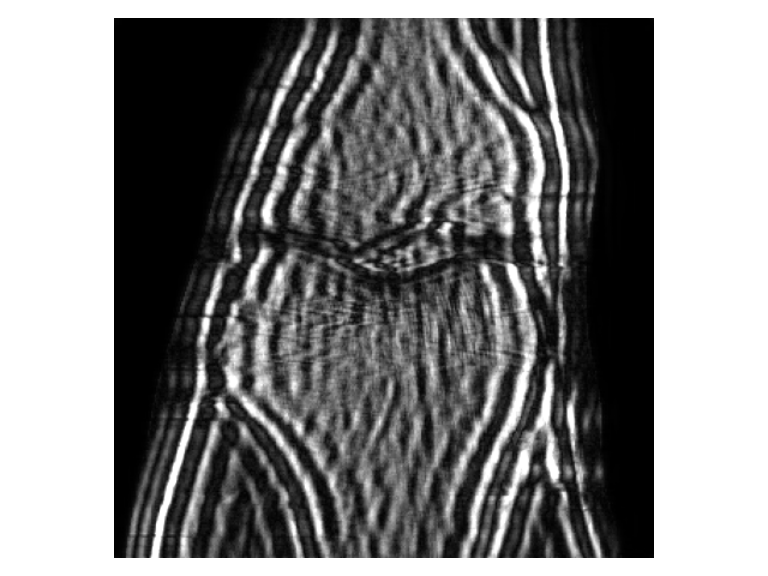
In Fig. 1-(a) and (b), we demonstrate an example of the reconstructed image $\mathbf{x}_{\text{{{MoDL}}}}$ from a benign input (i.e., clean and unperturbed input) and a PGD attacked input, respectively. As we can see, the quality of reconstructed image significantly degrades in the presence of adversarial (very small) input perturbations. Although robustness against adversarial attacks is a primary focus of this work, Fig. 1-(c) and (d) show two other types of instabilities that MoDL may suffer at testing time: the change of the measurement sampling rate (which leads to ‘perturbations’ to the sparsity of sampling mask in $\mathbf{A}$ ) [10], and the number of unrolling steps [12] used in MoDL for test-time image reconstruction. We observe that a over sampling mask (Fig. 1-(c)) and a larger number of unrolling steps (Fig. 1-(d)), which deviate from the training-time setting of MoDL, can lead to much poorer image reconstruction performance than the original setup (Fig. 1-(a)) even in the absence of an adversarial input. In Sec. 4, we will show that our proposed approach (originally designed for improving MoDL’s robustness against adversarial attacks) yields resilient reconstruction performance against all perturbation types shown in Fig. 1.

Refer to caption — Figure 1: MoDL’s instabilities against perturbations to input data, the measurement sampling rate, and the number of unrolling steps used at testing time shown on an image from the fastMRI [22] dataset. We refer readers to Sec. 4 for more experiment details. (a) MoDL reconstruction from benign (i.e., clean) measurement with $4\times$ acceleration (i.e., 25% sampling rate) and 8 unrolling steps. (b) MoDL reconstruction from adversarial input of perturbation strength $\epsilon=0.002$ (other settings are same as (a)). (c) MoDL reconstruction from clean measurement with $2\times$ acceleration (i.e., 50% sampling rate) and using 8 unrolling steps. (d) MoDL reconstruction from clean measurement with $4\times$ acceleration and using 16 unrolling steps.

Randomized smoothing (RS). RS creates multiple random noisy copies of input data and takes an averaged output over these noisy inputs so as to gain robustness against input noises [15]. Formally, given a base function $f(\mathbf{x})$ , RS turns this base function to a smoothing version $g(\mathbf{x})\mathrel{\mathop{:}}=\mathbb{E}_{\bm{\nu}\sim\mathcal{N}(\mathbf{0},\sigma^{2}\mathbf{I})}[f(\mathbf{x}+\bm{\nu})]$ , where $\bm{\nu}\sim\mathcal{N}(\mathbf{0},\sigma^{2}\mathbf{I})$ denotes the Gaussian distribution with zero mean and $\sigma^{2}$ -valued variance. In the literature, RS has been used as an effective adversarial defense in image classification [15, 16, 23]. However, it remains elusive whether or not RS is an effective solution to improving robustness of MoDL and other image reconstructors. A preliminary study towards this direction was provided by [18], which integrates RS with image reconstruction in an end-to-end (E2E) manner. For MoDL, this yields

\displaystyle g(\mathbf{A}^{H}\mathbf{y})=\mathbb{E}_{\bm{\nu}\sim\mathcal{N}(\mathbf{0},\sigma^{2}\mathbf{I})}[{\mathbf{x}}_{\text{{MoDL}}}(\mathbf{A}^{H}\mathbf{y}+\bm{\nu})].

(RS-E2E)

Fig. 2 provides an illustration of RS-E2E-baked MoDL. Although RS-E2E renders a simple application of RS to MoDL, it remains unclear if RS-E2E is the most effective way to bake RS into MoDL, considering the latter’s learning specialities, e.g., the involved denoising step and the DC step. In the rest of the paper, we will focus on studying two main questions (Q1)–(Q2).

3 SMUG: SMoothed UnrollinG

In this section, we tackle the above problems (Q1)–(Q2) by taking the unrolling characteristics of MoDL into the design of a RS-based robust MRI reconstruction. The proposed novel integration of RS with MoDL is termed Smoothed Unrolling (SMUG).

3.1 Solution to (Q1): RS at intermediate unrolled denoisers

Recall from Fig. 2 that the RS operation is applied to MoDL in an end-to-end fashion. Yet, the vanilla MoDL framework consists of multiple unrolling steps, each of which is naturally dissected into a ① denoising block (denoted by $\mathcal{D}$ ) and a ② DC block (denoted by $\mathcal{D}\mathcal{C}$ ). Taking the above architecture into account, RS can also be integrated with each intermediate unrolling step of MoDL instead of following RS-E2E. This leads to two new smoothing architectures of MoDL:

(a) SMUGv0: In this scheme, the RS operation is incorporated into MoDL at each unrolled step (i.e., $\mathrm{RS}(\mathcal{D}+\mathcal{DC})$ ). Formally, at the $n$ th step, we have $\mathrm{RS}(\mathcal{D}+\mathcal{DC})=\mathbb{E}_{\bm{\nu}\sim\mathcal{N}(\mathbf{0},\sigma^{2}\mathbf{I})}[{\mathbf{x}}_{n}(\mathbf{x}_{n-1}+\bm{\nu})]$ , where ${\mathbf{x}}_{n}(\mathbf{x}_{n-1}+\bm{\nu})$ denotes the output of the $n$ th unrolling step given the input $\mathbf{x}_{n-1}$ with Gaussian random noise $\bm{\nu}$ . Fig. 3-(a) provides a schematic overview of SMUGv0.

(b) SMUG: Different from SMUGv0, SMUG only applies RS to the denoising network, leading to $\mathrm{RS}(\mathcal{D})$ at each unrolling step. However, this seemingly simple modification aligns with a robustness certification technique, called ‘denoised smoothing’ [16], where a smoothed denoiser prepended to a victim model is sufficient to achieve provable robustness for this model. Formally, at the $n$ th unrolling step, we have

\displaystyle\mathrm{RS}(\mathcal{D})=\mathbb{E}_{\bm{\nu}\sim\mathcal{N}(\mathbf{0},\sigma^{2}\mathbf{I})}[\mathcal{D}_{\bm{\theta}}(\mathbf{x}_{n-1}+\bm{\nu})]\mathrel{\mathop{:}}=\mathbf{z}_{n},

(4)

together with the standard DC step $\mathbf{x}_{n+1}=\argmin_{\mathbf{x}}\|\mathbf{A}\mathbf{x}-\mathbf{y}\|^{2}_{2}+\lambda\|\mathbf{x}-\mathbf{z}_{n}\|_{2}^{2}$ . Fig. 3-(b) shows the architecture of SMUG.

As will be evident later, our empirical results in Sec. 4 (e.g., Fig. 4) show that SMUG and SMUGv0 can significantly outperform RS-E2E in adversarial robustness. In particular, SMUG achieves the best robust performance without sacrificing its standard accuracy when evaluated on benign testing data.

3.2 Solution to (Q2): SMUG’s pre-training and fine-tuning

In what follows, we develop the training scheme of SMUG. Spurred by the currently celebrated ‘pre-training + fine-tuning’ technique [19, 16], we propose to train the SMUG model following this learning paradigm. Our rationale is that pre-training is able to provide a robustness-aware initialization of the DL-based denoising network for ease of fine-tuning. To pre-train the denoising network $\mathcal{D}_{\bm{\theta}}$ , we consider a mean squared error (MSE) loss that measures the Euclidean distance between images denoised by $\mathcal{D}_{\bm{\theta}}$ and the labels (i.e., target images, denoted by $\mathbf{t}$ ). This leads to the pre-training step:

\bm{\theta}_{\mathrm{pre}}=\displaystyle\argmin_{\bm{\theta}}\mathbb{E}_{\mathbf{t}\in\mathcal{D}}[\mathbb{E}_{\bm{\nu}}||\mathcal{D}_{\bm{\theta}}(\mathbf{t}+\nu)-\mathbf{t}||_{2}^{2}]

(5)

where $\mathcal{D}$ denotes the set of labels, $\bm{\nu}\sim\mathcal{N}(0,\sigma^{2}I)$ . Note that the MSE loss (5) does not engage the entire unrolled network. Thus, the pre-training is computational inexpensive and time-efficient.

We next develop the fine-tuning scheme to improve $\bm{\theta}_{\mathrm{pre}}$ based on labeled MRI datasets, i.e., with access to target images (denoted by $\mathbf{t}$ ). Since RS in SMUG (Fig. 3-(b)) is applied to every unrolling step, we propose an unrolled stability (UStab) loss for fine-tuning the denoiser $\mathcal{D}_{\bm{\theta}}$ :

\displaystyle\ell_{\mathrm{UStab}}(\bm{\theta};\mathbf{y},\mathbf{t})=\sum_{n=0}^{N-1}\mathbb{E}_{\bm{\nu}}||\mathcal{D}_{\bm{\theta}}(\mathbf{x}_{n}+\bm{\nu})-\mathcal{D}_{\bm{\theta}}(\mathbf{t})||^{2}_{2},

(6)

where $N$ is the total number of unrolling steps, $\mathbf{x}_{0}=\mathbf{A}^{H}\mathbf{y}$ , and $\bm{\nu}\sim\mathcal{N}(0,\sigma^{2}I)$ . The UStab loss (6) relies on target images, bringing in a key benefit: the denoising stability is guided by the reconstruction accuracy of the ground-truth image, yielding a graceful tradeoff between robustness and accuracy.

Integrating the UStab loss (6) with the vanilla reconstruction loss of MoDL [3], we obtain the fine-tuned $\bm{\theta}$ by using

\displaystyle\ell(\bm{\theta};\mathbf{y},\mathbf{t})=\lambda_{\ell}\|\mathbf{x}_{N}(\bm{\theta};\mathbf{A}^{H}\mathbf{y})-\mathbf{t}\|_{2}^{2}+\ell_{\mathrm{UStab}}(\bm{\theta};\mathbf{y},\mathbf{t}),

(7)

where $\mathcal{D}$ denotes the labeled dataset, $\mathbf{x}_{N}$ is the reconstructed image using RS-applied MoDL (i.e., SMUGv0 and SMUG) with the denoising network of parameters $\bm{\theta}$ and input $\mathbf{A}^{H}\mathbf{y}$ , and $\lambda_{\ell}>0$ is a regularization parameter to strike the balance between reconstruction error (for accuracy) and denoising stability (for robustness). We fine-tune $\bm{\theta}$ using $\bm{\theta}_{\mathrm{pre}}$ as initialization.

4 Experiments

4.1 Experiment setup

Models & datasets. The studied RS-baked MoDL architectures are shown in Figs. 2 and 3. In experiments, we set the total number of unrolling steps to $N=8$ , and set the denoising regularization parameter $\lambda=1$ in vanilla MoDL. For the denoising network $\mathcal{D}_{\bm{\theta}}$ , we use the Deep Iterative Down-Up Network (DIDN) [24] with three down-up blocks and 64 channels. We adopt the conjugate gradient method [3] with tolerance $1e^{-6}$ to implement the DC block. We conduct our experiments on the fastMRI dataset [22]. The observed data $\mathbf{y}$ are obtained with $15$ coils and are cropped to the resolution of $320\times 320$ for MRI reconstruction. To implement the observation model, we adopt a Cartesian mask at $4\times$ acceleration (i.e., $25\%$ sampling rate). The coil sensitivity maps for all cases were obtained using the BART toolbox [25].

Training & evaluation. We use 304 images for training, 32 images for validation, and 64 images for testing (that are unseen during training). At training time, the batch size is set to $2$ trained on two GPUs. We use the the Adam optimizer to train studied MRI reconstruction models with the momentum parameters $(0.5,0.999)$ . The number of epochs is set to $60$ with a linearly decaying learning rate from $10^{-4}$ to $0$ after epoch 20. The stability parameter $\lambda_{\ell}$ in (7) is tuned so that the standard accuracy of the learned model is comparable to the vanilla MoDL. In RS, we set the standard deviation of Gaussian noise as $\sigma=0.01$ , and use $10$ Monte Carlo samplings to implement the smoothing operation. At testing time, we evaluate our methods on clean data, random noise-injected data and adversarial examples generated by 10-step PGD attack [10] of $\ell_{\infty}$ -norm radius $\epsilon=0.004$ . The quality of reconstructed images is measured using peak signal-to-noise ratio (PSNR) and structure similarity (SSIM). In addition to adversarial robustness, we also evaluate the performance of our methods at the presence of another two perturbation sources (i.e., altered sampling rate and unrolling step number at testing time), as shown in Fig. 6.

Table 1: Accuracy performance of different smoothing architectures (RS-E2E, SMUGv0, SMUG), together with the vanilla MoDL. Here ‘Clean Accuracy’, ‘Noise Accuracy’, and ‘Robust Accuracy’ refer to PSNR/SSIM evaluated on benign data, random noise-injected data, and PGD attack-enabled adversarial data, respectively.

\uparrow

signifies that a higher number indicates a better reconstruction accuracy. The result

a

\pm b

represents mean

a

and standard deviation

b

over 64 testing images. The relative performance is reported with respect to that of vanilla MoDL.

Models	Clean Accuracy		Noise Accuracy		Robust Accuracy
Metrics	PSNR $\uparrow$	SSIM $\uparrow$	PSNR $\uparrow$	SSIM $\uparrow$	PSNR $\uparrow$	SSIM $\uparrow$
Vanilla MoDL	29.73 $\pm$ 3.27	0.900 $\pm$ 0.07	28.70 $\pm$ 2.77	0.874 $\pm$ 0.07	22.91 $\pm$ 2.42	0.729 $\pm$ 0.07
RS-E2E	+0.09 $\pm$ 3.24	+0.002 $\pm$ 0.07	+0.38 $\pm$ 2.90	+0.010 $\pm$ 0.07	+0.78 $\pm$ 2.70	+0.034 $\pm$ 0.08
SMUGv0	-1.01 $\pm$ 3.07	-0.014 $\pm$ 0.08	-0.09 $\pm$ 2.99	+0.008 $\pm$ 0.08	+3.08 $\pm$ 2.42	-0.014 $\pm$ 0.11
SMUG (ours)	-0.34 $\pm$ 3.06	-0.006 $\pm$ 0.08	+0.53 $\pm$ 2.98	+0.016 $\pm$ 0.08	+3.87 $\pm$ 2.28	+0.008 $\pm$ 0.11

4.2 Experiment results

Figure 4: PSNR of baseline methods and proposed SMUG versus perturbation strength

\epsilon

used in PGD attack-generated adversarial examples at testing time. The case of

\epsilon=0

corresponds to clean accuracy.

Table 1 shows PSNR and SSIM values for different smoothing architectures with different training schemes, along with vanilla MoDL as a baseline, evaluated on clean and adversarial test datasets. We present the PSNR results for these models under different scales of adversarial perturbations (i.e., attack strength $\epsilon$ ) in Fig. 4. We observe that our method SMUG outperforms all other models in robustness, consistent with the visualization of reconstructed images in Fig. 5. Also, SMUG yields a promising clean accuracy performance, which is better than SMUGv0 and comparable to the vanilla MoDL model. This shows the effectiveness of our proposed method for improving robustness while preserving clean accuracy (i.e., without the perturbations).

Next, we evaluate the effectiveness of MRI reconstruction methods when facing sampling rate and unrolling step perturbations at testing time. In other words, there exists a test-time shift for the training setup of MRI reconstruction. In Fig. 6, we present the evaluation results of SMUG, with two baselines, vanilla MoDL and RS-E2E, on different unrolling steps and sampling rates. Note that these models are trained with the number of unrolling steps $K=8$ and sampling masks with the $4\times$ acceleration (i.e., 25% sampling rate). As we can see, SMUG achieves a remarkable improvement in robustness against different sampling rates and unrolling steps, which MoDL and RS-E2E fail to achieve. Although we do not intentionally design our method to mitigate MoDL’s instabilities against perturbed sampling rate and unrolling step number, SMUG still provides improved PSNRs over other baselines. We credit the improvement to the close relationships between these two instabilities with adversarial robustness.

Figure 6: PSNR results of different MRI reconstruction methods versus different measurement sampling rates (

4\times

acceleration i.e.,

25\%

sampling rate at training; Left plot) and unrolling steps (8 at training; Right plot).

Figure 7: PSNR vs. adversarial attack strength (

\epsilon)

of SMUG for different configurations of UStab loss (6).

We conduct additional experiments showing the importance of integrating target image denoising into SMUG’s training pipeline in (6). Fig. 7 shows PSNR versus perturbation strength ( $\epsilon$ ) when using different alternatives to $\mathcal{D}_{\bm{\theta}}(\mathbf{t})$ in (6), including $\mathbf{t}$ (the original target image), $\mathcal{D}_{\bm{\theta}}(\mathbf{x}_{n})$ (denoised output of each unrolling step), and their variants when using the fixed, vanilla MoDL’s denoiser $\mathcal{D}_{\bm{\theta}_{\text{{MoDL}}}}$ instead. As we can see, the performance of SMUG varies when the UStab loss (6) is configured differently. The proposed $\mathcal{D}_{\bm{\theta}}(\mathbf{t})$ outperforms the other baselines. A possible reason is that it infuses supervision of target images in an adaptive, denoising-friendly manner, i.e., taking influence of $\mathcal{D}_{\bm{\theta}}$ into consideration.

5 Conclusion

In this work, we proposed a scheme for improving robustness of DL-based MRI reconstruction. We showed deep unrolled reconstruction’s (MoDL’s) weaknesses in robustness against adversarial perturbations, sampling rates, and unrolling steps. To improve the robustness of MoDL, we proposed SMUG with a novel unrolled smoothing loss. Compared to the vanilla MoDL approach and several variants of SMUG, we empirically showed that our approach is effective and can significantly improve the robustness of MoDL against a diverse set of external perturbations. In the future, we will study the problem of certified robustness and derive the certification bound of adversarial perturbations using randomized smoothing.

References

[1] Michael Lustig, David L Donoho, et al., “Compressed sensing mri,” IEEE signal processing magazine, 2008.
[2] Junfeng Yang, Yin Zhang, and Wotao Yin, “A fast alternating direction method for tvl1-l2 signal reconstruction from partial fourier data,” IEEE Journal of Selected Topics in Signal Processing, 2010.
[3] Hemant K. Aggarwal, Merry P. Mani, and Mathews Jacob, “MoDL: Model-based deep learning architecture for inverse problems,” IEEE Trans. Med. Imaging, vol. 38, no. 2, pp. 394–405, Feb. 2019.
[4] Jo Schlemper, Chen Qin, Jinming Duan, Ronald M Summers, and Kerstin Hammernik, “Sigma-net: Ensembled iterative deep neural networks for accelerated parallel MR image reconstruction,” arXiv preprint arXiv:1912.05480, 2019.
[5] Saiprasad Ravishankar, Anish Lahiri, Cameron Blocker, and Jeffrey A Fessler, “Deep dictionary-transform learning for image reconstruction,” in 2018 IEEE 15th International Symposium on Biomedical Imaging (ISBI 2018). IEEE, 2018, pp. 1208–1212.
[6] Jo Schlemper, Jose Caballero, Joseph V. Hajnal, Anthony N. Price, and Daniel Rueckert, “A deep cascade of convolutional neural networks for dynamic MR image reconstruction,” IEEE Trans. Med. Imaging, vol. 37, no. 2, pp. 491–503, Feb. 2018.
[7] O. Ronneberger, P. Fischer, and T. Brox, “U-net: Convolutional networks for biomedical image segmentation,” in Medical Image Computing and Computer-Assisted Intervention – MICCAI 2015, 2015, pp. 234–241.
[8] Yoseob Han and Jong Chul Ye, “Framing u-net via deep convolutional framelets: Application to sparse-view ct,” IEEE T MED IMAGING, 2018.
[9] Dongwook Lee, Jaejun Yoo, et al., “Deep residual learning for accelerated mri using magnitude and phase networks,” IEEE Transactions on Biomedical Engineering, 2018.
[10] Vegard Antun, Francesco Renna, Clarice Poon, Ben Adcock, and Anders C Hansen, “On instabilities of deep learning in image reconstruction and the potential costs of ai,” Proceedings of the National Academy of Sciences, 2020.
[11] Chi Zhang, Jinghan Jia, et al., “On instabilities of conventional multi-coil mri reconstruction to small adverserial perturbations,” arXiv preprint arXiv:2102.13066, 2021.
[12] Davis Gilton, Gregory Ongie, and Rebecca Willett, “Deep equilibrium architectures for inverse problems in imaging,” IEEE Transactions on Computational Imaging, vol. 7, pp. 1123–1133, 2021.
[13] Aleksander Madry, Aleksandar Makelov, Ludwig Schmidt, Dimitris Tsipras, and Adrian Vladu, “Towards deep learning models resistant to adversarial attacks,” arXiv preprint arXiv:1706.06083, 2017.
[14] Hongyang Zhang, Yaodong Yu, Jiantao Jiao, Eric P Xing, Laurent El Ghaoui, and Michael I Jordan, “Theoretically principled trade-off between robustness and accuracy,” International Conference on Machine Learning, 2019.
[15] Jeremy Cohen, Elan Rosenfeld, and Zico Kolter, “Certified adversarial robustness via randomized smoothing,” in International Conference on Machine Learning. PMLR, 2019, pp. 1310–1320.
[16] Hadi Salman, Mingjie Sun, Greg Yang, Ashish Kapoor, and J Zico Kolter, “Denoised smoothing: A provable defense for pretrained classifiers,” Advances in Neural Information Processing Systems, vol. 33, 2020.
[17] Yimeng Zhang, Yuguang Yao, Jinghan Jia, Jinfeng Yi, Mingyi Hong, Shiyu Chang, and Sijia Liu, “How to robustify black-box ml models? a zeroth-order optimization perspective,” arXiv preprint arXiv:2203.14195, 2022.
[18] Adva Wolf, “Making medical image reconstruction adversarially robust,” 2019.
[19] Barret Zoph, Golnaz Ghiasi, Tsung-Yi Lin, Yin Cui, Hanxiao Liu, Ekin Dogus Cubuk, and Quoc Le, “Rethinking pre-training and self-training,” Advances in Neural Information Processing Systems, vol. 33, 2020.
[20] D.L. Donoho, “Compressed sensing,” IEEE Transactions on Information Theory, vol. 52, no. 4, pp. 1289–1306, 2006.
[21] Ian Goodfellow, Jonathon Shlens, and Christian Szegedy, “Explaining and harnessing adversarial examples,” 2015 ICLR, vol. arXiv preprint arXiv:1412.6572, 2015.
[22] Jure Zbontar, Florian Knoll, Anuroop Sriram, Tullie Murrell, Zhengnan Huang, Matthew J Muckley, Aaron Defazio, Ruben Stern, Patricia Johnson, Mary Bruno, et al., “fastmri: An open dataset and benchmarks for accelerated mri,” arXiv preprint arXiv:1811.08839, 2018.
[23] Yimeng Zhang, Yuguang Yao, Jinghan Jia, Jinfeng Yi, Mingyi Hong, Shiyu Chang, and Sijia Liu, “How to robustify black-box ML models? a zeroth-order optimization perspective,” in International Conference on Learning Representations, 2022.
[24] Songhyun Yu, Bumjun Park, and Jechang Jeong, “Deep iterative down-up cnn for image denoising,” in Proceedings of the IEEE/CVF Conference on Computer Vision and Pattern Recognition Workshops, 2019, pp. 0–0.
[25] Jonathan I Tamir, Frank Ong, Joseph Y Cheng, Martin Uecker, and Michael Lustig, “Generalized magnetic resonance image reconstruction using the berkeley advanced reconstruction toolbox,” in ISMRM Workshop on Data Sampling & Image Reconstruction, Sedona, AZ, 2016.


(a) Ground Truth	(b) Vanilla MoDL	(c) RS-E2E	(d) SMUG

SMUG: Towards Robust MRI Reconstruction by Smoothed UnrollingThanks: 1The work is done during remote internship at MSU.