Two-photon Hong-Ou-Mandel interference and quantum entanglement between the frequency-converted idler photon and the signal photonJournal: opticajournal

Optical frequency up-conversion has been the subject of much interest and investigation since its discovery in 1967 by Midwinter and Warner [1]. The driving factor behind the importance of up-conversion [2] has been the possibility of detecting infrared radiation [3, 4, 5, 6, 7] by converting it to the optical domain as the detection technology in the optical domain is much better. Thus, techniques for improving the efficiency of the up-conversion process have been developed [8, 9]. The improved efficiency is important for many applications, for example, in imaging [10, 11]. Of particular importance in the context of quantum technologies is the up-conversion of a single photon. The quantum theory of the up-conversion process has been developed [12, 13]. With the growing interest in quantum entanglement, Kumar and coworkers [14, 15, 8] demonstrated preservation of the quantum correlations between up-converted idler photons and signal photons produced by an optical parametric amplifier. In particular, they showed the survival of the non-classical intensity correlation between two photons at 1064 nm when one of these was converted to 532 nm. Since these early experiments, the interest shifted to single photons, and several experiments studied the quality of the up-converted single photons [16, 17] and verified the preservation of quantum correlations during the process [18, 19, 20]. As known, a versatile source of single photons is the spontaneous parametric down-conversion process where one has entangled pairs, i.e., signal and idler photons whose frequencies can be quite different, still exhibiting strong second-order quantum correlations represented by $g^{(2)}(\tau)$. Direct measurement of $g^{(2)}(\tau)$ is difficult as the correlation time could be 100 fs or less, and one uses the second-order Hong-Ou-Mandel interference [21, 22, 23, 24, 25, 26, 27, 28] for getting information at these time scales. In a recent work [29, 30] the correlation time was about 80 ps [31], and the frequency of the idler photon was up-converted by about 120 THz. Tyumenev et al [29] demonstrated the preservation of such correlation time between the up-converted idler photon and the signal photon. Given the considerable interest in the quantum properties of the up-converted photons, we present a first principle theoretical calculation of the non-classical time correlations of the up-converted and down-converted photon and the signal photon. We find the preservation of such correlations under fairly general conditions. We also analyze the two-photon Hong-Ou-Mandel interference between the frequency-converted idler photon and the signal photon. The visibility of the two-photon interference is sensitive to the magnitude of the frequency conversion, and it improves when the frequency separation between two photons goes down. Our theoretical results on HOM interference are quite relevant to several experiments, for example, [18, 19, 20] on the quality of frequency-converted single photons. Our results also apply to cases when the frequency is down-converted though we focus on up-conversion processes.

As shown in Fig. 1, we start with the entangled biphoton state [32] comprised of a idler photon of frequency $\omega_{s}$ and an signal photon of frequency $\omega_{i}$

$\displaystyle\ket{\Phi}=\int\int d\omega_{s}d\omega_{i}f(\omega_{s},\omega_{i})a_{s}^{\dagger}(\omega_{s})a_{i}^{\dagger}(\omega_{i})\ket{0,0},$

(1)

where $a_{s(i)}^{\dagger}(\omega_{s(i)})$ is the creation operator for the idler (signal) mode that satisfies the $[a_{s(i)}(\omega),a^{\dagger}_{s(i)}(\omega^{\prime})]=\delta(\omega-\omega^{\prime})$, and $[a_{s(i)}(\omega),a_{i(s)}(\omega^{\prime})]=[a_{s(i)}(\omega),a^{\dagger}_{i(s)}(\omega^{\prime})]=0$. Function $f(\omega_{s},\omega_{i})$ is the two-mode frequency distribution. We consider the input photon statistics to be an entangled Gaussian distribution

$\displaystyle f(\omega_{s},\omega_{i})=\frac{1}{\sqrt{2\pi\sigma_{P}\sigma_{-}}}e^{-(\omega_{s}+\omega_{i}-\omega_{p})^{2}/(16\sigma_{P}^{2})}e^{-(\omega_{s}-\omega_{i}-\triangle)^{2}/(4\sigma_{-}^{2})},$

(2)

where $\omega_{p}$ and $\sigma_{P}$ are the frequency and bandwidth of the pump; $\triangle$ is the frequency difference between the central frequency $\omega_{i0}$ and $\omega_{s0}$; $\sigma_{-}$ is the bandwidth of the photon pairs. The distribution is normalized, i.e., $\int\int|f(\omega_{s},\omega_{i})|^{2}d\omega_{s}d\omega_{i}=1$.

As for the frequency up-conversion process, The idler photon travels through a medium that up-shifts its frequency

$\displaystyle b_{i}(\omega)=T(\omega,\Omega)a_{i}(\omega-\Omega)+\eta(\omega,\Omega)a_{v}(\omega),$

(3)

where $T(\omega,\Omega)$ is the up-conversion rate; $a_{v}(\omega)$ is the vacuum noise creation operator and $\eta(\omega,\Omega)=\sqrt{1-|T(\omega,\Omega)|^{2}}$. The operators $b_{i}(\omega)$ and $b^{\dagger}_{i}(\omega^{\prime})$ satisfy the commutation relations $[b_{i}(\omega),b^{\dagger}_{i}(\omega^{\prime})]=\delta(\omega-\omega^{\prime})$. This formula has the same format as a transmission output-input relationship in an ordinary sample, while now the only difference is that the output frequency is up-converted, and the conversion rate should be dependent on both the original frequency and the frequency shift. Many experiments on frequency conversion use modulation at frequency $\Omega$. Thus the input photons at $\omega$ would be converted to $\omega+\Omega$ and $\omega-\Omega$. The modulation was in the GHz domain for some of the experiments, as noted in the introduction. The signal photon frequency remains the same. A phase shift is introduced due to the different paths taken by the photon pair

$\displaystyle b_{s}(\omega)=a_{s}(\omega)e^{-i\omega\tau_{0}}.$

(4)

The second order correlation $g^{(2)}(t,t+\tau)$ is defined as

$\displaystyle g^{(2)}(t,t+\tau)=\expectationvalue{b^{\dagger}_{i}(t)b^{\dagger}_{s}(t+\tau)b_{s}(t+\tau)b_{i}(t)}.$

(5)

Considering Eq. (1), (3), (4), we obtain

	$\displaystyle b_{s}(t+\tau)b_{i}(t)\ket{\Phi}$	$\displaystyle=\frac{1}{2\pi}\int\int d\omega_{1}d\omega_{2}T(\omega_{1},\Omega)a_{s}(\omega_{2})a_{i}(\omega_{1}-\Omega)e^{i\omega_{1}t}e^{i\omega_{2}(t+\tau-\tau_{0})}$
		$\displaystyle\times\int\int d\omega_{s}d\omega_{i}f(\omega_{s},\omega_{i})a_{s}^{\dagger}(\omega_{s})a_{i}^{\dagger}(\omega_{i})\ket{0,0},$		(6)

which gives the result for Eq. (5) as

$\displaystyle g^{(2)}(t,t+\tau)$

$\displaystyle=\frac{1}{4\pi^{2}}|\int\int d\omega_{1}d\omega_{2}T(\omega_{1},\Omega)\times e^{i\omega_{1}t}e^{i\omega_{2}(t+\tau-\tau_{0})}f(\omega_{1}-\Omega,\omega_{2})|^{2}.$

(7)

Note that the vacuum noise term does not contribute to the normal-ordered correlation. Assuming that the phase-matching is satisfied over the entire frequency width of the idler photon, then the up-conversion rate is a constant $T(\omega,\Omega)=T$ in the range of interest. Applying the parameter transformation $\Omega_{1}=\omega_{1}-\Omega$, Eq. (7) can be simplified to

$\displaystyle g^{(2)}(t,t+\tau)$

$\displaystyle=\frac{T^{2}}{4\pi^{2}}|\int\int d\Omega_{1}d\omega_{2}e^{i\Omega_{1}t}e^{i\omega_{2}(t+\tau-\tau_{0})}f(\Omega_{1},\omega_{2})|^{2}.$

(8)

Considering a photon pair following Gaussian distribution as in Eq. (2), we obtain

	$\displaystyle g^{(2)}(t,t+\tau)$	$\displaystyle=\frac{T^{2}}{(2\pi)^{3}\sigma_{P}\sigma_{-}}|\int\int d\Omega_{1}d\omega_{2}e^{i(\omega_{2}+\Omega_{1})\frac{(t+\tau^{\prime}-\tau_{0})+t}{2}}$
		$\displaystyle\times e^{i(\omega_{2}-\Omega_{1})\frac{(t+\tau-\tau_{0})-t}{2}}e^{-\frac{(\omega_{2}+\Omega_{1}-\omega_{p})^{2}}{16\sigma_{P}^{2}}}e^{-\frac{(\omega_{2}-\Omega_{1}-\triangle)^{2}}{4\sigma_{-}^{2}}}|^{2}.$		(9)

By orthogonally transforming parameters to $u=\frac{\omega_{2}+\Omega_{1}}{\sqrt{2}}$ and $v=\frac{\omega_{2}-\Omega_{1}}{\sqrt{2}}$, the double integral reduces to a product of two single-parameter integrals.

$\displaystyle g^{(2)}(t,t+\tau)$

$\displaystyle=\frac{T^{2}}{(2\pi)^{3}\sigma_{P}\sigma_{-}}|\int due^{iu\frac{2t+\tau-\tau_{0}}{\sqrt{2}}}e^{-(u-\frac{\omega_{p}}{\sqrt{2}})^{2}/(8\sigma_{P}^{2})}\int dve^{iv\frac{\tau-\tau_{0}}{\sqrt{2}}}e^{-(v-\frac{\triangle}{\sqrt{2}})^{2}/(2\sigma_{-}^{2})}|^{2}.$

Notably, the two integrals present in the expression are the Fourier transforms of Gaussian functions. The shifts $\frac{\omega_{p}}{\sqrt{2}}$ and $\frac{\triangle}{\sqrt{2}}$ thus don’t contribute to the modulus square. We then obtain

$\displaystyle g^{(2)}(t,t+\tau)=\frac{2\sigma_{P}\sigma_{-}T^{2}}{\pi}e^{-2\sigma_{P}^{2}(2t+\tau-\tau_{0})^{2}}e^{-\frac{1}{2}\sigma_{-}^{2}(\tau-\tau_{0})^{2}}.$

(11)

Note that $\omega_{p}$ and $\triangle$ do not explicitly contribute to the formula. This observation is due to the fact that the photon pair in question follows a standard bivariate normal distribution $f_{XY}(x,y)$. The correlation between the two variables, denoted by $\rho$, is described by the given formula [33, 34]

$\displaystyle f_{XY}(x,y)=\frac{1}{2\pi\sqrt{1-\rho^{2}}}e^{-\frac{x^{2}-2\rho xy+y^{2}}{2(1-\rho^{2})}}.$

(12)

In our case the correlation $\frac{4\sigma_{p}^{2}-\sigma_{-}^{2}}{4\sigma_{p}^{2}+\sigma_{-}^{2}}$ for the photon statistics $|f(\omega_{s},\omega_{i})|^{2}$ is a function of $\sigma_{-}$ and $\sigma_{p}$ only.

The two-time correlation in Eq. (11) is to be averaged over the resolution time $T_{R}$ of the detector.

$\displaystyle g^{(2)}(\tau)=\int_{-T_{R}/2}^{+T_{R}/2}dtg_{2}(t,t+\tau),$

(13)

which gives

$\displaystyle g^{(2)}(\tau)=\frac{1}{2\sqrt{2\pi}}\sigma_{-}T^{2}e^{-\frac{1}{2}\sigma_{-}^{2}(\tau-\tau_{0})^{2}}[erf(\sqrt{2}\sigma_{P}(\tau-\tau_{0}+T_{R}))-erf(\sqrt{2}\sigma_{P}(\tau-\tau_{0}-T_{R}))],$

where $erf(x)$ stands for the error function. We consider two scenarios. In the first scenario, when the large-detection time condition is satisfied, i.e., $\sigma_{P}T_{R}\rightarrow\infty$ and $T_{R}\gg\tau-\tau_{0}$, say with $T_{R}\sim 10\>ps$ or $100\>ps$, we obtain

$\displaystyle g^{(2)}(\tau)=\frac{\sigma_{-}T^{2}}{\sqrt{2\pi}}e^{-\frac{1}{2}\sigma_{-}^{2}(\tau-\tau_{0})^{2}}.$

(15)

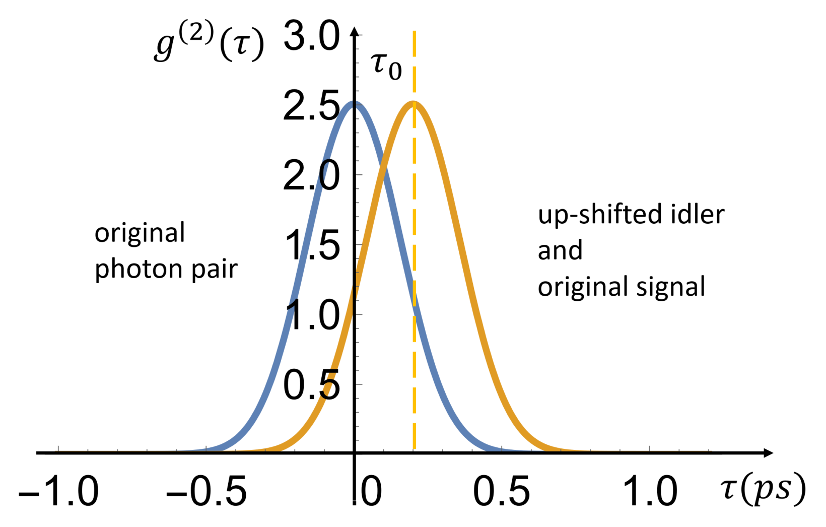
The FWHM of $g^{(2)}(\tau)$ between the up-shifted idler and original signal photon pair is the same as that between the original photon pairs. This is illustrated in Fig. 2, where the normalized $g^{(2)}(\tau)$ (by dropping the factor $T^{2}$) is plotted for the up-shifted idler and original signal photon pair, and demonstrates the presence of only a peak shift arising from the difference in path length. Note that Fig. 2 is obtained by using the exact result in Eq. (14). In the second scenario, $\sigma_{P}T_{R}\rightarrow 0$, and $\sigma_{P}(\tau-\tau_{0})\rightarrow 0$ we obtain

$\displaystyle g^{(2)}(\tau)=\frac{T_{R}\sigma_{P}\sigma_{-}T^{2}}{\sqrt{\pi}}e^{-\frac{1}{2}\sigma_{-}^{2}(\tau-\tau_{0})^{2}}.$

(16)

In both limits, the width of the $g^{(2)}(\tau)$ function is unchanged except for the phase difference imparted by the up-conversion medium from the correlation when there is no up-conversion (and no $\tau_{0}$).

$\displaystyle g^{(2)}_{0}(\tau)\propto\frac{\sigma_{-}}{\sqrt{2\pi}}e^{-\frac{1}{2}\sigma_{-}^{2}(\tau)^{2}}.$

(17)

Next, we examine the effect of phase-matching on the two-photon correlation. For this purpose, we now take the factor $T(\omega,\Omega)$ as

$\displaystyle T(\omega,\Omega)=Te^{-\frac{(\omega-\omega_{i0})^{2}}{2\beta^{2}}},$

(18)

where the conversion rate has a maximum at $\omega_{i0}$ to achieve maximum conversion. It decreases significantly outside the range indicated by $\beta$. We update Eq. (11) and (14) to

$\displaystyle g^{(2)}(t,t+\tau)=\frac{4T^{2}\beta^{2}\sigma_{P}\sigma_{-}}{\pi(2\beta^{2}+4\sigma_{P}^{2}+\sigma_{-}^{2})}e^{-\frac{\Omega^{2}+16\sigma_{P}^{2}\sigma_{-}^{2}(t+\tau-\tau_{0})^{2}+8\beta^{2}\sigma_{P}^{2}(2t+\tau-\tau_{0})^{2}+2\beta^{2}\sigma_{-}^{2}(\tau-\tau_{0})^{2}}{2(2\beta^{2}+4\sigma_{P}^{2}+\sigma_{-}^{2})}},$

(19)

and

	$\displaystyle g^{(2)}(\tau)=\frac{T^{2}\beta^{2}\sigma_{-}}{\sqrt{2\pi(2\beta^{2}+4\sigma_{P}^{2}+\sigma_{-}^{2})(\sigma_{-}^{2}+2\beta^{2})}}e^{-\frac{\Omega^{2}}{2(2\beta^{2}+4\sigma_{P}^{2}+\sigma_{-}^{2})}}e^{-\frac{4(\tau-\tau_{0})^{2}\beta^{2}\sigma_{-}^{2}\sigma_{P}^{2}}{(2\beta^{2}+4\sigma_{P}^{2}+\sigma_{-}^{2})(\sigma_{-}^{2}+2\beta^{2})}}e^{-\frac{\beta^{2}\sigma_{-}^{2}(\tau-\tau_{0})^{2}}{(2\beta^{2}+4\sigma_{P}^{2}+\sigma_{-}^{2})}}$
	$\displaystyle\times\{erf[\sqrt{\frac{2(\sigma_{-}^{2}+2\beta^{2})}{2\beta^{2}+4\sigma_{P}^{2}+\sigma_{-}^{2}}}(2\tau-2\tau_{0}+T_{R})]-erf[\sqrt{\frac{2(\sigma_{-}^{2}+2\beta^{2})}{2\beta^{2}+4\sigma_{P}^{2}+\sigma_{-}^{2}}}(2\tau-2\tau_{0}-T_{R})]\}.$		(20)

The expressions (19) and (20) reduce to equations (11) and (14) for $\beta^{2}\rightarrow\infty$. If the condition $T_{R}\gg(\tau-\tau_{0})$ is satisfied, then

$\displaystyle g^{(2)}(\tau)\propto e^{-\frac{\Omega^{2}}{2(2\beta^{2}+4\sigma_{P}^{2}+\sigma_{-}^{2})}}e^{-\frac{\beta^{2}\sigma_{-}^{2}}{(\sigma_{-}^{2}+2\beta^{2})}(\tau-\tau_{0})^{2}},$

(21)

showing explicit dependence on the parameter $\beta$ and the frequency change $\Omega$.

The Hong–Ou–Mandel (HOM) interferometer [21, 35, 36], a widely used tool in measuring biphoton joint frequency distribution, especially for time scales of 10’s of fs [37, 38, 39, 40]. We, therefore, study the two-photon interference between the up-converted idler and the signal photon. By introducing a tunable phase $\tau_{T}$ in the path of the signal photon, as depicted in Fig. 3, it is possible to measure both the frequency shift $\Omega$ and phase shift $\tau_{0}$ in a single setup. For the signal photon,

$\displaystyle b_{s}(\omega)=a_{s}(\omega)e^{-i\omega(\tau_{T}+\tau_{0})},$

(22)

while the idler photon travels through the same up-conversion medium. After frequency conversion, the two photons are recombined at a 50:50 beam-splitter. The output of the beam-splitter is expressed as

	$\displaystyle c(\omega)=\frac{b_{i}(\omega)+ib_{s}(\omega)}{\sqrt{2}},$
	$\displaystyle d(\omega)=\frac{ib_{i}(\omega)+b_{s}(\omega)}{\sqrt{2}}.$		(23)

As a result, the averaged coincidence rate of the output fields

$\displaystyle R_{c}(\tau_{T})=\frac{1}{4\pi^{2}}\int dt\int d\tau\expectationvalue{d^{\dagger}(t)c^{\dagger}(t+\tau)c(t+\tau)d(t)}$

(24)

is measured, where we assume the detection time is much larger than the pump correlation time $1/\sigma_{p}$ and the entanglement time $1/\sigma_{-}$. Changing the modes to the frequency domain $d(t)=\frac{1}{\sqrt{2\pi}}\int d\omega_{1}d(\omega_{1})e^{-i\omega_{1}t}$ and $c(t+\tau)=\frac{1}{\sqrt{2\pi}}\int d\omega_{2}c(\omega_{2})e^{-i\omega_{2}(t+\tau)}$, we obtain

	$\displaystyle R_{c}(\tau_{T})=\frac{1}{8\pi^{2}}$	$\displaystyle[\int\int d\omega_{1}d\omega_{2}f^{*}(\omega_{1}-\Omega,\omega_{2})f(\omega_{1}-\Omega,\omega_{2})T^{*}(\omega_{1},\Omega)T(\omega_{1},\Omega)$
	$\displaystyle-\int\int$	$\displaystyle d\omega_{1}d\omega_{2}f^{*}(\omega_{1}-\Omega,\omega_{2})f(\omega_{2}-\Omega,\omega_{1})T^{*}(\omega_{1},\Omega)T(\omega_{2},\Omega)e^{-i(\omega_{1}-\omega_{2})(\tau_{T}+\tau_{0})}].$

For a system with the same constant conversion rate assumption and photon distribution as in Eq. (2), we obtain

$\displaystyle R_{c}(\tau_{T})=\frac{T^{2}}{8\pi^{2}}(1-e^{-\frac{(\Omega-\triangle)^{2}}{2\sigma_{-}^{2}}}e^{-\frac{1}{2}\sigma_{-}^{2}(\tau_{T}+\tau_{0})^{2}}).$

(26)

The FWHM of $R_{c}(\tau_{T})$ is the same as the simple $g^{(2)}$ function as in Eq. (15), (16). The position of the peak in the HOM dip provides information on the phase difference, while the visibility $e^{-\frac{(\Omega-\triangle)^{2}}{2\sigma_{-}^{2}}}$ of the dip reveals the frequency shift $\Omega$. As shown in Fig. 4, the visibility of the HOM dip increases if the frequency difference between the signal and idler photons decreases due to the frequency conversion. Note that Eq. (26) shows that the visibility of the HOM dip remains sufficient as long as the parameter $f=\frac{\Omega-\triangle}{\sigma_{-}}\lesssim 1$, which is the case for reported experiments [18, 19, 20].

Next, we examine the effects of imperfect phase-matching in up-conversion using Eq. (18) and Eq. (25); we obtain

	$\displaystyle R_{c}(\tau_{T})$	$\displaystyle=\frac{\sqrt{2}T^{2}\beta}{8\pi^{2}}[\frac{1}{\sqrt{4\sigma_{P}^{2}+\sigma_{-}^{2}+2\beta^{2}}}e^{-\frac{2\Omega^{2}}{4\sigma_{P}^{2}+\sigma_{-}^{2}+2\beta^{2}}}$
		$\displaystyle-\frac{\beta}{\sqrt{(\beta^{2}+2\sigma_{P}^{2})(2\beta^{2}+\sigma_{-}^{2})}}e^{-\frac{(\Omega+\triangle)^{2}}{4(\beta^{2}+2\sigma_{P}^{2})}}e^{-\frac{(\Omega-\triangle)^{2}}{2\sigma_{-}^{2}}}e^{-\frac{\sigma_{-}^{2}\beta^{2}(\tau_{T}+\tau_{0})^{2}}{2\beta^{2}+\sigma_{-}^{2}}}],$		(27)

which reduces to Eq. (26) for $\beta^{2}\rightarrow\infty$. Note that Eq. (27) shares the same FWHM as Eq. (21). From Eq. (27), we obtain the visibility of the HOM dip

$\displaystyle V=\frac{\beta\sqrt{4\sigma_{P}^{2}+\sigma_{-}^{2}+2\beta^{2}}}{\sqrt{(\beta^{2}+2\sigma_{P}^{2})(2\beta^{2}+\sigma_{-}^{2})}}e^{-\frac{(\Omega+\triangle)^{2}}{4(\beta^{2}+2\sigma_{P}^{2})}}e^{-\frac{(\Omega-\triangle)^{2}}{2\sigma_{-}^{2}}}e^{\frac{2\Omega^{2}}{4\sigma_{P}^{2}+\sigma_{-}^{2}+2\beta^{2}}}.$

(28)

The visibility is maximized when $\Omega=\triangle$ as

$\displaystyle V=\frac{\beta\sqrt{4\sigma_{P}^{2}+\sigma_{-}^{2}+2\beta^{2}}}{\sqrt{(\beta^{2}+2\sigma_{P}^{2})(2\beta^{2}+\sigma_{-}^{2})}}e^{-\frac{(8\sigma_{P}^{2}+\sigma_{-}^{2}+4\beta^{2})\Omega^{2}}{(4\sigma_{P}^{2}+\sigma_{-}^{2}+2\beta^{2})(\beta^{2}+2\sigma_{P}^{2})}}.$

(29)

When $\beta\gg\sigma_{-}$ and $\sigma_{P}$, the visibility $V\rightarrow 1$. However, a very satisfactory visibility of 0.96 can be obtained when $\beta\sim 2\sigma_{-}$ for a system as shown in Fig. 5(a). The FWHM depends both on $\sigma_{-}$ and $\beta$. As shown in Fig. 5(b), when $\beta\sim 2\sigma_{-}$ the peak is only expanded by 50% compared to the value when $\beta\gg\sigma_{-}$.

The results of our theoretical study provide a comprehensive insight into the effect of frequency up-conversion on the time-dependent quantum correlation of a photon pair. By deriving the second-order correlation function, we demonstrate that the full width at half maximum (FWHM) remains unchanged, while the peak height and position shift after the up-conversion procedure. This finding agrees with the recent experiment [29], where the correlation time was within reach of the detector resolution time. This is true if the phase matching is satisfied over the spectral width of the idler photon. To gain a deeper understanding of the impact of the frequency up-conversion on the quantum correlation, we examined the two-photon Hong-Ou-Mandel interferometry. We showed how the visibility of the two-photon interference was sensitive to the magnitude of the frequency change in the up-conversion process, the bandwidth of the signal photon, and the phase matching factor $\beta$. These results are fairly general and are expected to apply to other types of frequency conversion.

JW and GSA thank the support of Air Force Office of Scientific Research (Award N^o FA-9550-20-1-0366) and the Robert A Welch Foundation (A-1943-20210327). AVS thanks Welch Foundation (Grant N^o A-1547) for support.

The authors declare no conflicts of interest.

No data were generated or analyzed in the presented research.

References

- [1] J. Midwinter and J. Warner, “Up-conversion of near infrared to visible radiation in lithium-meta-niobate,” Journal of Applied Physics 38, 519–523 (1967).
- [2] L. Ma, O. Slattery, and X. Tang, “Single photon frequency up-conversion and its applications,” Physics Reports 521, 69–94 (2012).
- [3] R. T. Thew, S. Tanzilli, L. Krainer, S. C. Zeller, A. Rochas, I. Rech, S. Cova, H. Zbinden, and N. Gisin, “Low jitter up-conversion detectors for telecom wavelength ghz qkd,” New Journal of Physics 8, 32 (2006).
- [4] A. P. Vandevender and P. G. Kwiat, “High efficiency single photon detection via frequency up-conversion,” Journal of Modern Optics 51, 1433–1445 (2004).
- [5] M. A. Albota and F. N. Wong, “Efficient single-photon counting at 1.55 m by means of frequency upconversion,” Optics Letters 29, 1449–1451 (2004).
- [6] C. Langrock, E. Diamanti, R. V. Roussev, Y. Yamamoto, M. M. Fejer, and H. Takesue, “Highly efficient single-photon detection at communication wavelengths by use of upconversion in reverse-proton-exchanged periodically poled linbo 3 waveguides,” Optics Letters 30, 1725–1727 (2005).
- [7] L. Ma, O. Slattery, and X. Tang, “Experimental study of high sensitivity infrared spectrometer with waveguide-based up-conversion detector,” Optics Express 17, 14395–14404 (2009).
- [8] Y.-P. Huang, V. Velev, and P. Kumar, “Quantum frequency conversion in nonlinear microcavities,” Optics Letters 38, 2119–2121 (2013).
- [9] S. Lefrancois, A. S. Clark, and B. J. Eggleton, “Optimizing optical bragg scattering for single-photon frequency conversion,” Phys. Rev. A 91, 013837 (2015).
- [10] A. Barh, P. J. Rodrigo, L. Meng, C. Pedersen, and P. Tidemand-Lichtenberg, “Parametric upconversion imaging and its applications,” Advances in Optics and Photonics 11, 952–1019 (2019).
- [11] A. Ashik, C. F. O’Donnell, S. C. Kumar, M. Ebrahim-Zadeh, P. Tidemand-Lichtenberg, and C. Pedersen, “Mid-infrared upconversion imaging using femtosecond pulses,” Photonics Research 7, 783–791 (2019).
- [12] W. H. Louisell, A. Yariv, and A. E. Siegman, “Quantum fluctuations and noise in parametric processes. i.” Phys. Rev. 124, 1646–1654 (1961).
- [13] J. Tucker and D. F. Walls, “Quantum theory of parametric frequency conversion,” Annals of Physics 52, 1–15 (1969).
- [14] P. Kumar, “Quantum frequency conversion,” Optics Letters 15, 1476–1478 (1990).
- [15] J. Huang and P. Kumar, “Observation of quantum frequency conversion,” Physical Review Letters 68, 2153 (1992).
- [16] H. J. McGuinness, M. G. Raymer, C. J. McKinstrie, and S. Radic, “Quantum frequency translation of single-photon states in a photonic crystal fiber,” Phys. Rev. Lett. 105, 093604 (2010).
- [17] S. Ates, I. Agha, A. Gulinatti, I. Rech, M. T. Rakher, A. Badolato, and K. Srinivasan, “Two-photon interference using background-free quantum frequency conversion of single photons emitted by an inas quantum dot,” Physical Review Letters 109, 147405 (2012).
- [18] L. Fan, C.-L. Zou, M. Poot, R. Cheng, X. Guo, X. Han, and H. X. Tang, “Integrated optomechanical single-photon frequency shifter,” Nature Photonics 10, 766–770 (2016).
- [19] C. Chen, J. E. Heyes, J. H. Shapiro, and F. N. Wong, “Single-photon frequency shifting with a quadrature phase-shift keying modulator,” Scientific Reports 11, 1–7 (2021).
- [20] D. Zhu, C. Chen, M. Yu, L. Shao, Y. Hu, C. Xin, M. Yeh, S. Ghosh, L. He, C. Reimer et al., “Spectral control of nonclassical light pulses using an integrated thin-film lithium niobate modulator,” Light: Science & Applications 11, 1–9 (2022).
- [21] C.-K. Hong, Z.-Y. Ou, and L. Mandel, “Measurement of subpicosecond time intervals between two photons by interference,” Physical Review Letters 59, 2044 (1987).
- [22] M. Barbieri, E. Roccia, L. Mancino, M. Sbroscia, I. Gianani, and F. Sciarrino, “What hong-ou-mandel interference says on two-photon frequency entanglement,” Scientific Reports 7, 1–6 (2017).
- [23] S. Walborn, A. De Oliveira, S. Pádua, and C. Monken, “Multimode hong-ou-mandel interference,” Physical Review Letters 90, 143601 (2003).
- [24] R.-B. Jin, R. Shiina, and R. Shimizu, “Quantum manipulation of biphoton spectral distributions in a 2d frequency space toward arbitrary shaping of a biphoton wave packet,” Optics Express 26, 21153–21158 (2018).
- [25] N. Fabre and S. Felicetti, “Parameter estimation of time and frequency shifts with generalized hong-ou-mandel interferometry,” Physical Review A 104, 022208 (2021).
- [26] T. Douce, A. Eckstein, S. P. Walborn, A. Z. Khoury, S. Ducci, A. Keller, T. Coudreau, and P. Milman, “Direct measurement of the biphoton wigner function through two-photon interference,” Scientific Reports 3, 1–6 (2013).
- [27] G. Boucher, T. Douce, D. Bresteau, S. P. Walborn, A. Keller, T. Coudreau, S. Ducci, and P. Milman, “Toolbox for continuous-variable entanglement production and measurement using spontaneous parametric down-conversion,” Physical Review A 92, 023804 (2015).
- [28] X. Liu, T. Li, J. Wang, M. R. Kamble, A. M. Zheltikov, and G. S. Agarwal, “Probing ultra-fast dephasing via entangled photon pairs,” Optics Express 30, 47463–47474 (2022).
- [29] R. Tyumenev, J. Hammer, N. Joly, P. S. J. Russell, and D. Novoa, “Tunable and state-preserving frequency conversion of single photons in hydrogen,” Science 376, 621–624 (2022).
- [30] A. V. Sokolov, “Giving entangled photons new colors,” Science 376, 575–576 (2022).
- [31] J. Hammer, M. V. Chekhova, D. R. Häupl, R. Pennetta, and N. Y. Joly, “Broadly tunable photon-pair generation in a suspended-core fiber,” Physical Review Research 2, 012079 (2020).
- [32] Y. Shih, An introduction to quantum optics: photon and biphoton physics (CRC press, 2020).
- [33] J. F. Kenney and E. S. Keeping, Mayhematics of Statistics (D. van Nostrand, 1939).
- [34] E. T. Whittaker and G. Robinson, The Calculus of Observations: a Treatise on Numerical Mathematics (Blackie and Son limited, 1924).
- [35] F. Bouchard, A. Sit, Y. Zhang, R. Fickler, F. M. Miatto, Y. Yao, F. Sciarrino, and E. Karimi, “Two-photon interference: the hong–ou–mandel effect,” Reports on Progress in Physics 84, 012402 (2020).
- [36] A. Hochrainer, M. Lahiri, M. Erhard, M. Krenn, and A. Zeilinger, “Quantum indistinguishability by path identity and with undetected photons,” Reviews of Modern Physics 94, 025007 (2022).
- [37] A. Lyons, G. C. Knee, E. Bolduc, T. Roger, J. Leach, E. M. Gauger, and D. Faccio, “Attosecond-resolution hong-ou-mandel interferometry,” Science advances 4, eaap9416 (2018).
- [38] G. Di Martino, Y. Sonnefraud, M. S. Tame, S. Kéna-Cohen, F. Dieleman, i. m. c. K. Özdemir, M. S. Kim, and S. A. Maier, “Observation of quantum interference in the plasmonic hong-ou-mandel effect,” Phys. Rev. Appl. 1, 034004 (2014).
- [39] B. Ndagano, H. Defienne, D. Branford, Y. D. Shah, A. Lyons, N. Westerberg, E. M. Gauger, and D. Faccio, “Quantum microscopy based on hong–ou–mandel interference,” Nature Photonics 16, 384–389 (2022).
- [40] A. Eshun, B. Gu, O. Varnavski, S. Asban, K. E. Dorfman, S. Mukamel, and T. Goodson III, “Investigations of molecular optical properties using quantum light and hong–ou–mandel interferometry,” Journal of the American Chemical Society 143, 9070–9081 (2021).