Abstract
The Unruh effect states that a uniformly linearly accelerated observer with proper acceleration experiences the Minkowski vacuum as a thermal state at temperature . An observer in uniform circular motion experiences a similar effective temperature, operationally defined in terms of excitation and de-excitation rates, and physically interpretable in terms of synchrotron radiation, but this effective temperature depends not just on the acceleration but also on the orbital speed and the excitation energy. In this paper we consider an observer in uniform circular motion when the Minkowski vacuum is replaced by an ambient thermal bath, and we address the interplay of ambient temperature, Doppler effect, acceleration, and excitation energy. Specifically, we consider a massless scalar field in spacetime dimensions, probed by an Unruh-DeWitt detector, in a Minkowski (rather than proper) time formulation: this setting describes proposed analogue spacetime systems in which the effect may become experimentally testable, and in which an ambient temperature will necessarily be present. We establish analytic results for the observer’s effective temperature in several asymptotic regions of the parameter space and provide numerical results in the interpolating regions, finding that an acceleration effect can be identified even when the Doppler effect dominates the overall magnitude of the response. We also identify parameter regimes where the observer sees a temperature lower than the ambient temperature, experiencing a cooling Unruh effect.
[Circular motion analogue Unruh effect in a thermal bath]Circular motion analogue Unruh effect in a thermal bath: Robbing from the rich and giving to the poor
Cameron R D Bunney and Jorma Louko
March 2023; revised May 2023.22 2 Published in Classical and Quantum Gravity 40, 155001 (2023), doi:10.1088/1361-6382/acde3b. For Open Access purposes, this Author Accepted Manuscript is made available under CC BY public copyright.
1 Introduction
The Unruh effect [1, 2, 3, 4] is a remarkable result in quantum field theory, stating that a uniformly linearly accelerated observer with proper acceleration in Minkowski spacetime reacts to a quantum field in its Minkowski vacuum through excitations and de-excitations with the characteristics of a thermal state, at the Unruh temperature , proportional to the acceleration. Direct experimental verification is still, however, unconfirmed. A large hurdle to overcome is the sheer magnitude of acceleration required to reach a detectable increase in temperature. Experimental confirmation retains broad interest in its relation to the Hawking effect [5], and the connections to the early universe quantum effects, which may originate the present-day structure of the Universe [6, 7].
Phenomena similar to the Unruh effect exist also for non-linear uniform motion [8, 9, 10], including uniform circular motion [11, 12, 13, 14, 15]. Experimental interest in the circular motion Unruh effect has a long standing [16, 17, 18, 19, 20, 21, 22], in which a new angle was opened by recent proposals [23, 24, 25, 26] to utilise the analogue spacetime that occurs in nonrelativistic laboratory systems [27, 28, 29].
In analogue spacetime, circular motion enjoys two main advantages over linear acceleration. First, the experiment can remain within a finite-size laboratory for an arbitrarily long interaction time. Second, the time dilation Lorentz factor between the laboratory and the accelerated worldline remains constant in time: this allows the inclusion of the time dilation gamma-factor by appropriately scaling the energies in the theoretical analysis of the experiment, without the need to engineer a time-dependent energy scaling in a condensed matter system. Notwithstanding these advantages, a complication in circular motion is that the linear acceleration Unruh temperature formula is no longer directly applicable, and the effective temperature, operationally defined in terms of excitation and de-excitation probabilities in the accelerating system, involves also dependency on the orbital speed and the excitation energy. The underlying reason for this is that the circular motion effect does not admit a description in terms of a genuine thermal equilibrium state adapted to the motion, but has instead a physical interpretation in terms of synchrotron radiation, as reviewed in [4]. A detailed comparison of the linear and circular acceleration Unruh temperatures in and spacetime dimensions is given in [30]. Related earlier analyses are given in [10, 12, 18, 19, 21, 31, 32].
In the conventional setting of the Unruh effect, the ambient quantum field is prepared in its Minkowski vacuum, with zero temperature — an idealisation that no experimental test of the effect would be able to completely mimic. The purpose of this paper is to address the circular motion Unruh effect when the ambient quantum field is prepared in a thermal state, with a positive ambient temperature. Related earlier analyses are given in [18, 19, 32, 33].
We assume the circular motion to have no drift in the rest frame of the ambient heat bath. The total system is then invariant under time translations along the trajectory, and the Unruh effect will be time independent. We further specialise to a massless scalar field in dimensions, and we probe the field with a pointlike Unruh-DeWitt (UDW) detector [3, 34]. Finally, whereas UDW detectors normally have their transition energies defined with respect to the relativistic proper time along the detector’s trajectory [3, 34], we define the transition energies with respect to the Minkowski time in the heat bath’s rest frame. This setting describes proposed analogue spacetime systems in which the effect may become experimentally testable, and in which an ambient temperature will necessarily be present [25, 26].
We work in linear perturbation theory in the coupling between the detector and the field, in the limit of long interaction time but negligible back-action. We do not address finite interaction time effects [35] or the back-action of the detector on the field [36].
A positive ambient temperature however brings up one new technical issue that needs to be addressed. The thermal Wightman function for a massless scalar field is well defined in spacetime dimensions [32] and higher, but in dimensions it is infrared divergent [12]. We sidestep this divergence by considering an UDW detector that couples linearly to the time derivative of the scalar field along the trajectory, rather than to the value of the field. The derivative-coupled detector is often employed to sidestep a similar infrared divergence that occurs for a massless field in spacetime dimensions already in zero temperature [37, 38, 39, 40, 41, 42].
We first obtain a mode sum expression for the response function of the UDW detector, allowing the field to have any dispersion relation subject to mild monotonicity assumptions. In the analogue spacetime setting, this allows field frequencies that go beyond the phononic regime [23, 28]; in a fundamental relativistic spacetime setting, this allows dispersion relations that might arise from Planck scale physics [43].
We then specialise to the massless Klein-Gordon field. We establish analytically the asymptotic behaviour of the response function in several regimes, including the low and high ambient temperature regimes, and the corresponding asymptotic behaviour of the effective temperature, defined operationally via the detailed balance relation between excitations and de-excitations. We present numerical results for the interpolating regimes, chosen for their potential relevance for prospective experiments [25, 26].
As a highlight, we show that an acceleration effect can be identified even when the Doppler effect dominates the overall magnitude of the detector’s response,as is expected to be the case in the Helium analogue spacetime system considered in [26]. We also identify regimes in which the detector experiences an effective temperature that is lower than the ambient temperature, so that the Unruh effect induces cooling rather than heating. Criteria by which the Unruh effect may be argued to induce cooling have been discussed in a variety of relativistic spacetime settings [44, 45, 46, 47, 48, 49, 50, 51, 52, 53, 54, 55, 56].
As a mathematical side outcome, we evaluate in closed form an infinite series (3.8) involving squared Bessel functions. We have not encountered this identity in the existing literature.
We begin in Section 2 by establishing the preliminaries for an UDW detector in uniform circular motion in -dimensional Minkowski spacetime, coupled to the time derivative of a quantised real scalar field that is prepared in a thermal state. We obtain a mode sum expression for the detector’s response function, recall the detailed balance definition of an effective temperature, reviewing its motivations and limitations, and we investigate general conditions under which the detailed balance temperature could be expected to be lower than the ambient temperature. We also present a corresponding discussion for an inertial detector at a constant velocity with respect to the heat bath.
Section 3 investigates analytically the detailed balance temperature in several limiting regimes of the parameter space, both for circular motion and for inertial motion. Interpolating numerical results are provided in Section 4. Separating the acceleration contribution from the Doppler contribution in the detector’s response is addressed in Section 5, by a combination of analytics and numerics. Section 6 presents a summary and concluding remarks. Proofs of technical results are deferred to two appendices.
We use units in which , where is the speed of light in the relativistic spacetime interpretation and the speed of sound in the analogue spacetime interpretation. Sans serif letters (x) denote spacetime points and boldface Italic letters () denote spatial vectors. In asymptotic formulae, denotes that remains bounded in the limit considered, and denotes that tends to zero in the limit considered.
2 Field and detector preliminaries
In this section we review the relevant background for an UDW detector on a circular trajectory in -dimensional Minkowski spacetime, coupled to a real scalar field in a thermal state. We work in the limit of weak coupling and long interaction time, with negligible back-action of the detector on the field. We recall how the detailed balance condition, relating the detector’s excitation and de-excitation rates, provides a notion of an effective temperature experienced by the detector, in general, dependent on the energy scale of the transitions. We also give an initial discussion about identifying regimes where the effective temperature might be lower than the ambient temperature. Finally, we present the response of a detector in inertial motion, in preparation for distinguishing effects due to acceleration from those due to speed.
2.1 Field and detector
We work in -dimensional Minkowski spacetime, with a standard set of Minkowski coordinates and the metric . In this spacetime we consider a quantised real scalar field , with a dispersion relation that is isotropic in and subject to the mild monotonicity conditions specified in Section 2.2, but otherwise arbitrary; in particular, we do not assume the dispersion relation to be Lorentz invariant. We denote by the standard Fock space in which the positive frequencies are defined with respect to the timelike Killing vector .
We assume that the field has been prepared in a thermal state in inverse temperature , where the notion of thermality is with respect to the time evolution generated by . We assume that the thermal state has a Wightman two-point function, denoted by
| (2.1) |
possibly modulo infrared subtleties that we shall describe shortly. is not invariant under Lorentz boosts, not even when the dispersion relation is Lorentz invariant, because of the role of in the construction of the state: a heat bath has a distinguished rest frame.
We probe the field by a pointlike detector in uniform circular motion, on the worldline
| (2.2) |
where is the orbital radius and is the angular velocity. The orbital speed is . We assume that the worldline is timelike, . We have parametrised the worldline by the Minkowski time because this will give us a detector response that is appropriate for describing an analogue spacetime system, where is the ‘lab time’ with respect to which any frequencies will be measured [25, 26, 30]. For a genuinely relativistic detector, whose microphysics operates according to the relativistic proper time, the worldline should be parametrised by the relativistic proper time.
The detector’s Hilbert space is , spanned by the orthonormal basis . The detector’s Hamiltonian , generating dynamics with respect to the Minkowski time , acts on as and , where . The detector is hence a two-level system, with energy gap : for , is the ground state and is the excited state; for , the roles are reversed. We have included in the symbol the overline to emphasise that this energy is defined with respect to the Minkowski time, and the notation is thus adapted to the analogue spacetime system, where is the distinguished ‘lab time’. The conversion to a relativistic detector is by , where is the energy with respect to the detector’s proper time and , and, for transition rates, by including the overall factor .
The total Hilbert space is .
In the interaction picture, and continuing to define time evolution with respect to the Minkowski time, we take the interaction Hamiltonian to be
| (2.3) |
where is the detector’s monopole moment operator, is a real-valued switching function that specifies how the interaction is turned on and off, and is a real-valued coupling constant. Working to first order in perturbation theory in , the probability for the detector to transition from to , regardless of the final state of the field, is [3, 57]
| (2.4) |
where is the response function, given by
| (2.5) |
and
| (2.6) |
As the factors in front of in (2.4) are constants, independent of , and the trajectory, we may, with a traditional abuse of terminology, refer to as the probability.
We refer to (2.6) as the derivative correlation function. Had (2.3) not included the time derivative, in (2.5) would have been replaced by the pullback of the Wightman function (2.1) to the detector’s worldline,
| (2.7) |
For a massless Klein-Gordon field, is however infrared divergent [12]. We shall see that including the time derivative in makes the detector’s response well defined even for the massless Klein-Gordon field.
As the thermal state is stationary with respect to the Killing vector and isotropic in , the Wightman function is invariant under time translations along the detector’s trajectory, so that . Dividing by the total duration of the interaction, and letting the duration tend to infinity, reduces to the stationary response function,
| (2.8) |
which is interpreted as the transition probability per unit time. The subtleties in the infinite duration limit are discussed in [35]; in particular, the limit assumes the coupling to tend to zero sufficiently fast for the first order perturbative treatment to remain valid in the limit.
From now on we work with the stationary response function (2.8), and we refer to it as the response function.
2.2 Response function mode sum
As the field’s dispersion relation is by assumption spatially isotropic, the field mode frequency with respect to can be written as , where is the spatial momentum and is function of a non-negative argument, positive everywhere except possibly at . We write , and we assume that for . Finally, if , we assume that .
We show in A that the response function has the mode sum expression
| (2.9) |
where
| (2.10) |
are the Bessel functions of the first kind [58], and is defined for , as the unique solution to
| (2.11) |
The uniqueness of follows from the positivity of , and the notation suppresses the -dependence of . Note that (2.10) is the Planckian factor characteristic of a thermal distribution in a bosonic field.
If , the factors have singularities, but, by the assumption , these singularities are more than outweighed by the factors for , whereas the term is not singular because by assumption; is hence continuous in , but it is not smooth. We shall comment on this in more explicitly with the massless Klein-Gordon field below.
2.3 Massless Klein-Gordon field
We now specialise to the massless Klein-Gordon field, for which , and . The response function (2.2) then simplifies to
| (2.12a) | ||||
| (2.12b) | ||||
| (2.12c) | ||||
where is the vacuum contribution, independent of , while is the additional contribution due to the ambient temperature. Note that is even in , and we have written (2.12c) in a way that makes this manifest. Note also that both and are manifestly positive.
Recall that by assumption and , where . It follows from the uniform asymptotic expansion 10.20.4 in [58] that the sums in (2.12b) and (2.12c) converge, and is hence well defined. is however not smooth in at integer values of , where new terms enter the sums: at , has a discontinuity in its derivative and has a discontinuity in its derivative.
2.4 Detailed balance temperature
We now describe the detailed balance temperature, an effective, energy-dependent notion of temperature, which we use to quantify the detector’s response.
2.4.1 Context
To set the context, recall that in a local system in equilibrium with a thermal bath,
the excitation and de-excitation probabilities satisfy Einstein’s detailed balance condition [59, 60],
| (2.14) |
where is the exitation probability, is the de-excitation probability, is the energy difference between the two states under consideration, and is the temperature of the thermal bath. Solving (2.14) for gives
| (2.15) |
which gives an operational way to determine the bath’s temperature in terms of the probabilities and that are observable in the local system. Note that while both and depend on , the temperature in (2.14) and (2.15) does not: the temperature sets the ratio of the excitation and de-exitation probabilities for all energy gaps. This is the characteristic feature of a local system in equilibrium with a thermal bath.
In the linear acceleration Unruh effect, the excitation and de-excitation probabilities of a localised detector obey the detailed balance condition (2.14) in the triple limit of weak coupling, long interaction time and sharp spatial localisation [3, 34]: is the energy gap defined with respect to the relativistic proper time, and given by (2.15) is the Unruh temperature, , where is the relativistic proper acceleration. The reason behind this phenomenon is that the Minkowski vacuum is a genuine thermal state in the Fock space adapted to the boost Killing vector whose one orbit the linearly-accelerated observer follows [3], and the detector consequently responds to this thermality by excitations and de-excitations that obey detailed balance. Subtleties in the sense of the triple limit of weak coupling, long interaction time and sharp spatial localisation are discussed in [35, 36, 61, 62].
For non-linear uniform accelerations, by contrast, Minkowski vacuum does not have a similar description as a genuine thermal state in a Fock space adapted to the accelerated motion. While the excitation and de-excitation probabilities are affected by the acceleration, the ratio of these probabilities depends on the energy gap in a way that does not follow the detailed balance exponential law (2.14), describable by the single parameter . The non-linear uniformly accelerated motions therefore do not have a conventional notion of temperature, and the physical phenomenon behind the acceleration effect may be described as a combination of synchrotron radiation and the conventional Unruh effect, as reviewed in [4]. In particular, the quantity given by (2.15) depends on the gap .
The probabilities and are however observable quantities in the local quantum system, affected by the acceleration, even when the acceleration is not linear. For a given value of , the excitation and de-excitation probabilities in the local system are related as if the system were in equilibrium with a thermal bath in the temperature given by (2.15). The -dependent quantity given by (2.15) provides thus a useful quantifier of the system’s response to the acceleration at energy gap , and hence an operational notion of an effective temperature at a given energy scale. We call this quantity the detailed balance temperature.
To summarise: for the non-linear uniform accelerations the detailed balance temperature does not arise from an underlying thermal bath, but it is a useful quantifier of the response of the local quantum system at a given energy scale. This is the sense in which we employ the detailed balance temperature in this paper.
2.4.2 Uniform circular motion
Returning to our uniform circular motion setting,
we define the detailed balance temperature by
| (2.16) |
where we recall that is the transition energy with respect to the Minkowski time (rather than the relativistic proper time), and the notation suppresses that may a priori depend on all the parameters of the problem, including . While can have either sign, the right-hand side of (2.16) is invariant under , so that depends on only through the gap magnitude . As positive (respectively negative) corresponds to an excitation (a de-excitation), we see that (2.16) agrees with (2.15), but with respect to Minkowski time rather than relativistic proper time.
We thus adopt the detailed balance temperature (2.16) as an effective temperature at the energy scale . The notions of heating and cooling used below will compare with the ambient temperature .
2.5 Cooling inequality
We shall find in Sections 3.1 and 4 that there are regimes where the circular motion detailed balance temperature is lower than the ambient temperature . Here we make preliminary observations as to where such parameter regimes might be found.
The definition (2.16) may be rearranged as
| (2.17) |
Whilst (2.17) holds for either sign of , let us assume here , for simplicity of the notation. As is by construction positive, (2.17) then shows that the condition for to be lower than is
| (2.18) |
Using (2.12), and the evenness of , this becomes
| (2.19) |
2.6 Inertial motion response function
In this subsection we record the response function of a detector that is in inertial motion but with a nonvanishing velocity with respect to the heath bath. We shall use this in the later sections to distinguish the acceleration contribution from the velocity contribution in the circular motion response.
Specialising to the massless Klein-Gordon field, the inertial motion response function may be obtained from (2.8) with (1.1) and (1.2) in a straightforward way, using identities and in [63]. The outcome is
| (2.20) |
where is the detector’s velocity in the heat bath’s rest frame, satisfying , and is the Lorentz factor. The subscript “Lin” stands for “linear”, emphasising that the inertial motion may be viewed as the limit of the circular motion (2.2) with fixed orbital speed ; as a consistency check, we have verified that (2.20) may be obtained from (2.12) in this limit, viewing the sum as the Riemann sum of an integral and using the asymptotic expansions of the Bessel functions [58]. The integrand in (2.20) is singular at the upper and lower limits, but these singularities are integrable and the integral is well defined.
3 Asymptotic regimes
In this section we find analytic expressions for the response and the detailed balance temperature for circular motion in the asymptotic regimes of high and low ambient temperature, small energy gap, small orbital radius with fixed speed, and near-sonic speed. We also give the corresponding results for inertial motion, including there also the regime of large energy gap. We demonstrate that for both circular motion and inertial motion there are regimes in which the detailed balance temperature is lower than the ambient temperature.
3.1 High ambient temperature
Consider the high ambient temperature limit, , with , and fixed.
By 24.2.1 in [58], the Planckian factor (2.10) has the small argument Laurent expansion
| (3.1) |
convergent for , where are the Bernoulli numbers. The Bessel function factors in (2.12c) have exponential decay at large , by 10.20.4 in [58]. It follows, by a dominated convergence argument, that the asymptotic expansion of at may be found from (2.12c) by using (3.1) under the sum over and reversing the order of the sums. The expansion proceeds in powers with , and to the leading order we have
| (3.2) |
For the detailed balance temperature, (2.12), (2.16), and (3.2) give
| (3.3) |
where
| (3.4) |
is assumed positive, and we recall that .
The function (3.4) is well defined. The sums over converge, by the exponential falloff seen from 10.20.4 in [58], and the denominator is positive, as is seen by writing the denominator as
| (3.5) |
using (2.12b) and (2.13). The positivity of (3.5) follows by breaking the integral into a sum of integrals over the intervals , , combining each even interval with the next odd interval, noting that the combined integrand in each term is then positive because the denominator in (3.5) is a strictly increasing function of , and finally observing that these rearrangements are justified by the convergence of (3.5) as an improper Riemann integral.
At small with fixed , has the asymptotic behaviour
| (3.6) |
as can be verified by expanding the sums in (3.4) in term by term; interchanging the sum and the expansion is justified because the falloff 10.20.4 in [58] allows differentiating the sums with respect to term by term for . It follows that for fixed , for sufficiently small .
At with fixed , tends to zero, decaying proportionally to . To see this, we note that the numerator in (3.4) remains bounded as , by 10.20.4 in [58], while the denominator diverges, with the leading term , as is seen using the integral representation (3.5) and the asymptotic expansion in Appendix E of [30].
Collecting these observations about , we see that for sufficiently high ambient temperatures, is lower than the ambient temperature for any fixed and sufficiently large , and also for any fixed and sufficiently small . We shall return to numerically in Section 4.
We note in passing that while the sums stemming from do not appear to have elementary analytic expressions, admits an elementary analytic bound at the special value , at the demarcation between the two asymptotic behaviours shown in (3.6): from (2.12c) we have
| (3.7) |
and the bound is sharper at lower values of . The inequality in (3.7) follows by renaming the summation index and replacing the Planckian factor by its value at the lowest summand, and the equality follows from the identity
| (3.8) |
which we verify in B. We have not found this identity in the existing literature.
3.2 Low ambient temperature
Consider the low ambient temperature limit, , with , and fixed.
The Planckian factor (2.10) has the large argument expansion
| (3.9) |
convergent for . By the exponential decay of the Bessel function factors in (2.12c), it follows by a dominated convergence argument that the asymptotic expansion of as may be found from (2.12c) by using (3.9) and rearranging the sums. We find
| (3.10) |
where
| (3.11) |
is the floor function, and the notation suppresses the -dependence of . Note that since
| (3.12) |
(3.10) shows that has an exponential decay in .
The dominant term of the exponential decay can be determined by analysing how the exponents in (3.10) depend on . There are three qualitatively different cases:
- 1.
For , :
(3.13) - 2.
For , :
(3.14) - 3.
For , :
(3.15)
The coefficient in the exponent of the large falloff is hence discontinuous in at integer values of , by (3.15). At half-integer values of , the coefficient in the exponent is continuous in , but the overall magnitude is discontinuous, by (3.14).
3.3 Small gap
Consider the limit , with fixed , and .
In (2.12c), for we have
| (3.16) |
using (3.1), and expanding in under the sum, justified by the falloff seen from 10.20.4 in [58].
3.4 Large gap
Consider the limit , with fixed , and .
For , using the integral representation (2.13) and adapting the analysis of [30] to our conventions shows that consists of the inertial motion contribution and a piece that is exponentially suppressed in .
Estimating (2.12c) at would require new techniques. We shall not pursue this estimate here.
3.5 Small radius with fixed speed
Consider the limit with fixed , and .
In (2.12c), writing gives, for ,
| (3.19) |
Note that both and remain finite as , despite the diverging acceleration.
3.6 Large radius with fixed speed
3.7 Machian limit
Consider the limit , with fixed , and . In terms of , this is the limit with fixed , and . In the analogue spacetime interpretation, this is the Machian, or near-sonic, limit.
In (2.12c), the -factors have an exponential large falloff, while the falloff of the Bessel function factors is exponential for and for , as seen from 10.20.4 in [58]. It follows that has a finite limit as ,
| (3.22) |
3.8 Inertial motion
In this subsection we record the corresponding asymptotic regime results for inertial motion.
For large/small and large/small , we use (2.21) and note that the expansions depend on and only through the combination . At high ambient temperature and/or small gap, , we find
| (3.26a) | ||||
| (3.26b) | ||||
using (3.1). At low ambient temperature and/or large gap, , we find
| (3.27a) | ||||
| (3.27b) | ||||
using (3.9) and the properties 10.32.1 and 10.40.1 from [58] of the modified Bessel function .
For the Machian limit, , we start from (2.20), change variables by , use a dominated convergence argument to take the limit under the integral, and use 25.12.11 in [58]. We find
| (3.28a) | ||||
| (3.28b) | ||||
where is the polylogarithm [58].
In the low ambient temperature and/or large gap regime, the detailed balance temperature is always higher than the ambient temperature, by (3.26b). However, in the high ambient temperature and/or small gap regime, the detailed balance temperature is always lower than the ambient temperature, by (3.27b), and similarly in the Machian limit, by (3.28b).
4 Numerical results
In this section we present numerical evidence about the detailed balance temperature in inertial motion and circular motion, interpolating between the asymptotic regimes considered in Section 3.
4.1 Detailed balance temperature in inertial motion
Consider first the inertial motion.
All the independent information in is obtained by expressing as a function of and by (2.16) and (2.21). A plot is shown in Figure 1. The plot displays the interpolation between the large heating effect (3.27b), the small cooling effect (3.26b) and the large cooling effect (3.28b).

4.2 Detailed balance temperature in circular motion
Consider now the circular motion.
As a preliminary, recall from (3.3) that the high ambient temperature asymptotics of is determined by the function (3.4), with . It was found in Section 3.1 that in this limit, there is a cooling effect for any fixed and sufficiently large , and also for any fixed and sufficiently small . The plot of in Figure 2 confirms numerically these analytic findings, and indicates that there is a cooling effect when for any , assuming the patterns in the plotted range continue outside the plotted range.
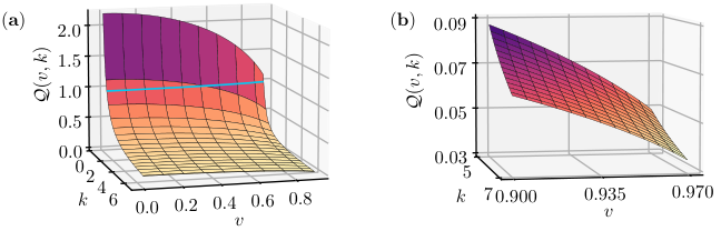

(b) As in (a), but showing the difference of the detailed balance temperature and the ambient temperature: the vertical axis is , where . Note that the horizontal axes in (a) and (b) increase in opposite directions, for the benefit of the visual perspective. The horizontal (blue) curve is at , at the boundary between a heating effect and a cooling effect, and the white curve at is at the discontinuity in the first derivative, as in (a). A cooling effect near sets in at moderate ambient temperature, from where it extends to high ambient temperature for .
Returning to finite ambient temperature, we address the interpolation between the asymptotic regimes analysed in Section 3 by plotting in Figure 3(a) the detailed balance temperature as a function of the ambient temperature and the energy gap, for fixed and a fixed orbital radius, and in Figure 3(b) the difference of the detailed balance temperature and the ambient temperature. The orbital radius enters the plots only in that it sets the scales of the axes, and the range of the variables is chosen to cover the main transitional region of interest and to indicate the onset of asymptotics as numerical efficacy allows.
The most prominent overall feature in Figure 3(a) is that the ambient temperature dominates when the ambient temperature is high, as was to be expected, and as is consistent with the analytic estimates of Section 3. The key information in Figure 3 is how the interpolation between the heating and cooling effects due to motion occurs: while we know from Section 3 and Figure 2 that a high ambient temperature cooling occurs for , Figure 3 shows that this cooling effect occurs already for moderate ambient temperature if .
5 Acceleration versus speed in circular motion
In this section we ask how much of the circular motion effect on the detector’s response can be attributed to the detector’s speed and how much to the acceleration.
5.1 Acceleration quantifiers
A primary quantity indicating the significance of acceleration is the difference of the circular motion and inertial motion transition rates at the same speed. We quantify this difference by the ratio
| (5.1) |
where the notation on the right-hand side suppresses that in is taken equal to in , and the notation on the left-hand side makes explicit that depends on the parameters only through the dimensionless triple , as seen from (2.12) and (2.21). In words, is the relative excess transition rate due to the acceleration at a given speed. Note that may a priori be positive or negative. The acceleration contribution is insignificant iff .
A secondary quantity indicating the significance of acceleration is the ratio of the circular motion detailed balance temperature to the inertial motion detailed balance temperature, , at the same speed. Like , depends on the parameters only through the dimensionless triple . Where is approximately unity, and where is it significantly different from unity?
5.2 Asymptotic regimes
We consider analytically four asymptotic regimes, using the results of Section 3.
First, in the limit with fixed , and , the trajectory becomes inertial, and the effects due to acceleration become insignificant by construction, as discussed in Section 3.6: we have and .
Second, consider the limit with fixed , and . From Sections 3.3 and 3.8 we obtain
| (5.2a) | ||||
| (5.2b) | ||||
The acceleration effect in the transition rate hence tends to zero linearly in , but with different coefficients for excitations and de-excitations. The acceleration effect in the detailed balance temperature however remains nontrivial in this limit, increasing the temperature from by the factor .
Third, consider the limit with fixed , and . From Sections 3.5 and 3.8 we find that both and have finite limits as , despite the diverging acceleration. The limits depend on the remaining variables only through the pair , but in a fairly complicated way: we find
| (5.3a) | ||||
| (5.3b) | ||||
using the large and small results from Section 3.8. The limit of takes hence a wide range of values, from much less than unity to much larger than unity, depending on . The limit of , by contrast, is larger than unity for both small and large , and much larger than unity for large .
5.3 Numerical results
We present numerical results for , plotting and as a function of the independent dimensionless variables and .


Figure 4 shows a plot of , both for , corresponding to excitations, and for , corresponding to de-excitations. In both cases, the plot indicates that for , but significant deviations start near , and there are regions of positive and regions of negative . We emphasise that the behaviour near is independent of the ambient temperature, and this behaviour hence occurs even when the ambient temperature is so high that the ambient temperature dominates the overall magnitude of the detector’s response. At , the behaviour in the plots is consistent with the asymptotic formulas given above.
Figure 5 shows a plot of , with the same parameter range as in Figure 4. is close to unity for , as had to happen by Figure 4, but it starts to deviate significantly from unity near , where in some regions but in some regions . The behaviour at is consistent with the asymptotic formulas given above.
In summary, the combination of numerical an analytic evidence indicates that the acceleration has a negligible effect on the transition rate and on the detailed balance temperature for , but nontrivial behaviour due to the acceleration occurs at .
6 Conclusions
Motivated by proposals to observe the analogue spacetime circular motion Unruh effect in condensed matter systems [23, 24, 25, 26], we have analysed finite ambient temperature effects on a pointlike quantum system in uniform circular motion in -dimensional Minkowski spacetime. We modelled the ambient quantum field by a massless Klein-Gordon field, prepared in a thermal state, and we modelled the pointlike quantum system by an UDW detector, coupled linearly to the time derivative of the field, where the time derivative is introduced to regularise an infrared divergence in the field’s thermal Wightman function. We specified the detector’s internal dynamics in terms of Minkowski time, instead of the detector’s relativistic proper time, as this is expected to be more closely connected to quantities measured in an analogue spacetime experiment. We worked in the limit of weak interaction and long interaction time and neglected the detector’s back-action on the field.
We quantified the detector’s response by an effective detailed balance temperature , computed from the detector’s excitation and de-excitation rates by the detailed balance formula (2.16), and interpretable as an effective temperature within a limited energy band. We obtained analytic results in several asymptotic regimes and numerical results in the interpolating regimes.
We found parameter regimes where is higher than the ambient temperature, so that the detector’s motion causes a heating effect, and parameter regimes where is lower than the ambient temperature, so that the detector’s motion causes a cooling effect. Comparing with an inertial detector, we found regimes where the heating/cooling is dominated by the detector’s speed with respect to the heat bath, due to the Doppler effect, and the acceleration has only a minor role; conversely, we found regimes where the acceleration in the detector’s motion is significant.
While the interplay of the various regimes is subtle, one general feature is that a cooling effect is more likely to occur when the ambient temperature is high, as one might have expected on qualitative grounds. Another feature is that the detector’s acceleration, rather than just the speed, is significant at energy gaps smaller than the orbital angular velocity, even when the ambient temperature is so high that the overall magnitude of the detector’s transition rate is dominated by the ambient temperature.
As a mathematical side product, we found an elementary expression for an infinite series (3.8) involving squared Bessel functions. We have not encountered this identity in the existing literature.
We recap that our motivation to consider a finite ambient temperature came from proposals to simulate an UDW detector on a circular orbit in a relativistic spacetime by a condensed matter system, such as a phonons in a Bose-Einstein condensate or third sound waves in superfluid Helium, with a laser beam playing the role of the detector [25, 26]. These condensed matter systems simulate a Klein-Gordon field in a relativistic spacetime when probed at at sufficiently low frequencies, but they can never simulate a field state with a strictly zero temperature, and controlling finite ambient temperature effects is crucial. Our results chart the parameter space for these ambient temperature effects. As mentioned above, a specific upshot is that even when the ambient temperature is so high that the overall magnitude of the detector’s response is dominated by the ambient temperature, as is likely be the case in superfluid Helium [26], the acceleration effect can be distinguished from a Doppler shift effect by focusing on detector energy gaps smaller than the orbital angular velocity. This will inform the design of prospective experiments as analysed in [26].
To summarise, an ambient temperature equips the circular motion Unruh effect with the characteristic of Robin Hood [64]: Where there is little, the Unruh effect gives; and where there is plenty, the Unruh effect takes.
Appendix A Response function mode sum
In this appendix we find the mode sum expression (2.2) for the response function. The notation and the assumptions are as in Section 2.2.
The positive Minkowski frequency mode functions of the massless Klein-Gordon field are
| (1.1) |
where is the spatial momentum and the dispersion relation (suppressed in the notation) specifies as a function of . The normalisation is , where is the Klein-Gordon inner product and is the Dirac delta. It follows as in [12] that the derivative correlation function (2.6) has the mode sum expression
| (1.2) |
where is the circular motion worldline (2.2), is the Planckian factor (2.10) and the asterisk denotes complex conjugation.
We substitute in (1.2) the mode functions (1.1) and the trajectory (2.2), perform the differentiations, and change the integration variables from to by a suitable (time-dependent) rotation in the plane, obtaining
| (1.3) |
where and is now a function of . An equivalent expression is
| (1.4) |
as can be seen by considering the difference of (1.3) and (1.4) and noting that the integral over the angle in the plane produces a sum of , and that vanishes by Bessel’s differential equation [58]. Note that the integrals in (1.3) and (1.4) are free of infrared divergences: when , this follows from the assumption .
We next use in (1.4) the identity
| (1.5) |
which follows from 10.12.1 in [58], and we regroup the sum so that all the -dependence is in factors of the form , multiplied by Bessel functions of order , and . We then convert the integral over and to polar coordinates by , so that . The odd terms are odd in and vanish on integration over . We relabel the even terms by with , substitute in(2.8), and perform the integral over in terms of delta-functions, which collapse the integral over , with the outcome
| (1.6) |
where are as defined in Section 2.2, and the notation suppresses their -dependence.
The integrals in (1.6) can be evaluated using the identities
| (1.7a) | ||||
| (1.7b) | ||||
| (1.7c) | ||||
where ; these identities follow from in [63] by setting respectively , and . Further use of Bessel function identities 10.6.1 and 10.6.2 in [58] then gives formula (2.2) in the main text.
We end this appendix with two comments on the role of the time derivatives in (2.2).
First, when , the result (2.2) can be obtained more shortly in the following way. The property implies that the non-derivative correlation function (2.7) is well defined, and (2.6) and (2.7) give . Using the time translation invariance of and , we then have
| (1.8) |
where the factor has come from integration by parts. The right-hand side of (1.8) is recognised as times the response function of a detector without a derivative in the coupling. We can now apply the methods of this appendix directly to the right-hand side of (1.8), arriving at (2.2) through significantly fewer steps: the overall factor in (2.2) is exactly the overall factor in (1.8).
Second, when , is infrared divergent, and (1.8) as it stands is not well defined. However, if we ignore the infrared divergence in the mode sum expression for , and informally apply to (1.8) the integral interchange manipulations of this appendix, we arrive again at (2.2): the informal integral interchanges can be interpreted as a regularisation of the infrared divergence in the transition rate. This regularisation of the transition rate can be applied even when the detector’s coupling does not involve a time derivative [33].
Appendix B Bessel function identity
In this appendix we verify the identity
| (2.1) |
where .
Proof.
The case is trivial as the only nonvanishing term on the left-hand side is . We henceforth assume .
References
References
- [1] Fulling S A 1973 Phys. Rev. D 7 2850–2862
- [2] Davies P C W 1975 J. Phys. A: Math. Gen. 8 609–616
- [3] Unruh W G 1976 Phys. Rev. D 14 870–892
- [4] Fulling S A and Matsas G E A 2014 Scholarpedia 9 31789
- [5] Hawking S W 1975 Commun. Math. Phys. 43 199–220 [Erratum: Commun. Math. Phys. 46, 206 (1976)]
- [6] Parker L 1969 Phys. Rev. 183 1057–1068
- [7] Mukhanov V and Winitzki S 2007 Introduction to Quantum Effects in Gravity (Cambridge University Press)
- [8] Letaw J R 1981 Phys. Rev. D 23 1709–1714
- [9] Korsbakken J I and Leinaas J M 2004 Phys. Rev. D 70 084016 (Preprint hep-th/0406080)
- [10] Good M, Juárez-Aubry B A, Moustos D and Temirkhan M 2020 JHEP 06 059 (Preprint 2004.08225)
- [11] Letaw J R and Pfautsch J D 1980 Phys. Rev. D 22 1345–1351
- [12] Takagi S 1986 Prog. Theor. Phys. Supp. 88 1–142
- [13] Doukas J and Carson B 2010 Phys. Rev. A 81 062320 (Preprint 1003.2201)
- [14] Jin Y, Hu J and Yu H 2014 Annals of Physics 344 97–104
- [15] Jin Y, Hu J and Yu H 2014 Phys. Rev. A 89 064101 (Preprint 1406.5576)
- [16] Bell J S and Leinaas J M 1983 Nuclear Physics B 212 131–150
- [17] Bell J S and Leinaas J M 1987 Nucl. Phys. B 284 488–508
- [18] Costa S S and Matsas G E A 1995 Phys. Rev. D 52 3466–3471 (Preprint gr-qc/9412030)
- [19] Guimaraes A C C, Matsas G E A and Vanzella D A T 1998 Phys. Rev. D 57 4461–4466 (Preprint hep-ph/9703309)
- [20] Leinaas J M 1999 Accelerated electrons and the Unruh effect 15th Advanced ICFA Beam Dynamics Workshop on Quantum Aspects of Beam Physics ed Chen P (World Scientific) pp 577–593 (Preprint hep-th/9804179)
- [21] Unruh W G 1998 Phys. Rept. 307 163–171 (Preprint hep-th/9804158)
- [22] Lochan K, Ulbricht H, Vinante A and Goyal S K 2020 Phys. Rev. Lett. 125 241301 (Preprint 1909.09396)
- [23] Retzker A, Cirac J I, Plenio M B and Reznik B 2008 Phys. Rev. Lett. 101 110402 (Preprint 0709.2425)
- [24] Marino J, Menezes G and Carusotto I 2020 Phys. Rev. Res. 2 042009 (Preprint 2001.08646)
- [25] Gooding C, Biermann S, Erne S, Louko J, Unruh W G, Schmiedmayer J and Weinfurtner S 2020 Phys. Rev. Lett. 125 213603 (Preprint 2007.07160)
- [26] Bunney C R D, Biermann S, Barroso V S, Geelmuyden A, Gooding C, Ithier G, Rojas X, Louko J and Weinfurtner S 2023 (Preprint 2302.12023)
- [27] Unruh W G 1981 Phys. Rev. Lett. 46 1351–1353
- [28] Barcelo C, Liberati S and Visser M 2005 Living Rev. Rel. 8 12 (Preprint gr-qc/0505065)
- [29] Volovik G 2009 The Universe in a Helium Droplet International Series of Monographs on Physics (Oxford University Press)
- [30] Biermann S, Erne S, Gooding C, Louko J, Schmiedmayer J, Unruh W G and Weinfurtner S 2020 Phys. Rev D 102 085006 (Preprint 2007.09523)
- [31] Müller D 1995 (Preprint gr-qc/9512038)
- [32] Hodgkinson L, Louko J and Ottewill A C 2014 Phys. Rev. D 89 104002 (Preprint 1401.2667)
- [33] Barman S, Majhi B R and Sriramkumar L 2022 (Preprint 2205.01305)
- [34] DeWitt B S 1979 Quantum Gravity: The New Synthesis General Relativity: An Einstein Centenary Survey ed Hawking S W and Israel W (Cambridge: Cambridge University Press) pp 680–745
- [35] Fewster C J, Juárez-Aubry B A and Louko J 2016 Class. Quantum Grav. 33 165003 (Preprint 1605.01316)
- [36] Lin S Y and Hu B L 2007 Phys. Rev. D 76 064008 (Preprint gr-qc/0611062)
- [37] Raine D J, Sciama D W and Grove P G 1991 Proc. R. Soc. Lond. A 435 205–215
- [38] Raval A, Hu B L and Anglin J 1996 Phys. Rev. D 53 7003–7019 (Preprint gr-qc/9510002)
- [39] Wang Q and Unruh W G 2014 Phys. Rev. D 89 085009 (Preprint 1312.4591)
- [40] Juárez-Aubry B A and Louko J 2014 Class. Quant. Grav. 31 245007 (Preprint 1406.2574)
- [41] Juárez-Aubry B A and Louko J 2018 JHEP 05 140 (Preprint 1804.01228)
- [42] Juárez-Aubry B A and Louko J 2022 AVS Quantum Sci. 4 013201 (Preprint 2109.14601)
- [43] Amelino-Camelia G 2013 Living Rev. Rel. 16 5 (Preprint 0806.0339)
- [44] Brenna W G, Mann R B and Martín-Martínez E 2016 Phys. Lett. B 757 307–311 (Preprint 1504.02468)
- [45] Liu P H and Lin F L 2016 JHEP 07 084 (Preprint 1603.05136)
- [46] Garay L J, Martín-Martínez E and de Ramon J 2016 Phys. Rev. D 94 104048 (Preprint 1607.05287)
- [47] Li T, Zhang B and You L 2018 Phys. Rev. D 97 045005 (Preprint 1802.07886)
- [48] Henderson L J, Hennigar R A, Mann R B, Smith A R H and Zhang J 2020 Phys. Lett. B 809 135732 (Preprint 1911.02977)
- [49] Pan Y and Zhang B 2020 Phys. Rev. A 101 062111 (Preprint 2009.05179)
- [50] Pan Y and Zhang B 2021 Phys. Rev. D 104 125014 (Preprint 2112.01889)
- [51] De Souza Campos L and Dappiaggi C 2021 Phys. Lett. B 816 136198 (Preprint 2009.07201)
- [52] Barman S and Majhi B R 2021 JHEP 03 245 (Preprint 2101.08186)
- [53] Zhou Y, Hu J and Yu H 2021 JHEP 09 088 (Preprint 2105.14735)
- [54] Robbins M P G and Mann R B 2022 Phys. Rev. D 106 045018 (Preprint 2107.01648)
- [55] Chen Y, Hu J and Yu H 2022 Phys. Rev. D 105 045013 (Preprint 2110.01780)
- [56] Wu S M, Zeng H S and Liu T 2022 New J. Phys. 24 073004 (Preprint 2207.01259)
- [57] Birrell N D and Davies P C W 1982 Quantum Fields in Curved Space Cambridge Monographs on Mathematical Physics (Cambridge University Press)
- [58] NIST Digital Library of Mathematical Functions http://dlmf.nist.gov/, Release 1.1.9 of 2023-03-15 F. W. J. Olver, A. B. Olde Daalhuis, D. W. Lozier, B. I. Schneider, R. F. Boisvert, C. W. Clark, B. R. Miller, B. V. Saunders, H. S. Cohl, and M. A. McClain, eds.
- [59] Einstein A 1917 Phys. Z. 18 121–128
- [60] ter Haar D 1967 The Old Quantum Theory (Elsevier)
- [61] Benatti F and Floreanini R 2004 Phys. Rev. A 70 012112
- [62] De Bièvre S and Merkli M 2006 Class. Quant. Grav. 23 6525–6542 (Preprint math-ph/0604023)
- [63] Gradshteyn I S and Ryzhik I M 2007 Table of Integrals, Series, and Products seventh ed (Elsevier/Academic Press, Amsterdam)
- [64] Weinfurtner S 2022 private communication