Enhanced Blackhole mergers in AGN discs due to Precession induced resonances
Abstract
Recent studies have shown that AGN discs can host sources of gravitational waves. Compact binaries can form and merge in AGN discs through their interactions with the gas and other compact objects in the disc. It is also possible for the binaries to shorten the merging timescale due to eccentricity excitation caused by perturbations from the supermassive blackhole (SMBH). In this paper we focus on effects due to precession-induced (eviction-like) resonances, where nodal and apsidal precession rates of the binary is commensurable with the mean motion of the binary around the SMBH. We focus on intermediate mass black hole (IMBH)-stellar mass black hole (SBH) binaries, and consider binary orbit inclined from the circum-IMBH disk which leads to the orbital precession. We show that if a binary is captured in these resonances and is migrating towards the companion, it can undergo large eccentricity and inclination variations. We derive analytical expressions for the location of fixed points, libration timescale and width for these resonances, and identified two resonances in the near coplanar regime (the evection and eviction resonances) as well as two resonances in the near polar regime that can lead to mergers. We also derive analytical expressions for the maximum eccentricity that a migrating binary can achieve for given initial conditions. Specifically, the maximum eccentricity can reach 0.9 when captured in these resonances before orbital decay due to gravitational wave emission dominates, and the capture is only possible for slow migration ( Myr) 2-3 order of magnitude longer than the resonance libration timescale. We also show that capture into multiple resonances is possible, and can further excite eccentricities.
Subject headings
hierarchical triple systems — secular dynamics — evection resonance — eviction resonanceI. Introduction
Multiple mechanisms have been proposed to account for the recent detections of gravitational waves. It has been suggested that the sources for these events could be merging compact objects in isolated binaries (Dominik et al. 2012; Kinugawa et al. 2014; Belczynski et al. 2016; Belczynski et al. 2018; Giacobbo et al. 2018; Spera et al. 2019; Bavera et al. 2020), isolated triple systems (Li et al. 2014; Hoang et al. 2018; Antonini et al. 2014; Silsbee & Tremaine 2017; Antonini et al. 2017) and star clusters (Banerjee 2017; O’Leary et al. 2006; Samsing et al. 2014; Rodriguez et al. 2016; Askar et al. 2017; Zevin et al. 2019; Di Carlo et al. 2019). Additionally, AGN discs which are dense with embedded stars and compact objects are also expected to be sources of gravitational waves. A wide variety of processes can aid in the merger of compact objects in AGN discs including flybys and gas dynamical friction (Bartos et al. 2017; Tagawa et al. 2020; Leigh et al. 2018; Stone et al. 2017; Tagawa et al. 2021).
More recently, it has been shown that migrating binary black holes in an AGN disc can be captured in evection resonances causing the eccentricity of the binary to be excited allowing the binaries to merge on a shorter timescale (Muñoz et al. 2022; Bhaskar et al. 2022). In this work, we explore other resonances which can also cause similar eccentricity excitation. In our previous paper (Bhaskar et al. 2022), we assumed a coplanar setup which allows resonances involving only the longitude of pericenter of the binary. In this work we relax that assumption allowing the binaries to have an arbitrary orientation with respect to the AGN disc, and for simplicity we now focus on IMBH-SBH binaries.
More specifically, in this paper we focus on resonances which occur when a linear combination of apsidal and nodal precession rates of the binary is commensurable with the mean motion of the companion. The most well studied of these resonances is the evection resonance which occurs when the precession rate of the longitude of pericenter of the binary equals the mean motion of the companion. Evection resonances have been shown to be important in many astrophysical systems. It was initially used to show that the Moon in it’s early evolution could have been trapped in evection resonance induced by the Sun, allowing the transfer of angular momentum from Earth-Moon orbit to Earth-Sun orbit (Touma & Wisdom 1998; Cuk et al. 2019; Tian et al. 2017). More recently, it has been shown that circumbinary planets with an external perturber (Xu & Lai 2016), binary blackholes in AGN discs (Bhaskar et al. 2022; Muñoz et al. 2022), multiplanet systems (Touma & Sridhar 2015) and satellites around exoplanets (Spalding et al. 2016; Cuk & Burns 2004) can be trapped in evection resonance. Other precession induced resonances have also been studied. For instance, Touma & Wisdom 1998 show that the moon could also have been trapped in Eviction resonance in the past. Additionally, Yoder 1982, Yokoyama 2002 and Vaillant & Correia 2022 explore the possibility of capture of moons of Mars and Neptune in other precession induced resonances .
Our main interest in studying these resonances is to explore the possibility of eccentricity excitation in binaries. While mechanisms which allow eccentricity excitation are of interest to many astrophysical systems, in this paper we focus on blackhole binaries in AGN disc. The paper is organized as follows: In §II, we develop the analytical theory for the system. We derive the Hamiltonian describing the dynamics of the system. In §II.2, we focus on the dynamics of binaries trapped in precession induced resonances. We derive analytical expressions for resonance location, libration timescale and resonant width at low eccentricity. We then describe our single-averaged simulations in §III. We apply our results to BBHs in AGN discs in §IV. We summarize our results and conclude in §V. Readers only interested in applications to AGN disks can skip §II and §III.
II. Analytical theory
II.1. Single averaged Hamiltonian
The schematic of the system is shown in Figure 1. It contains a binary comprising of objects with masses and being orbited by a third object with mass on a wider orbit. We define an inner orbit tracking the evolution of masses and around each other and an outer orbit tracking the evolution of the outer companion () around the center of mass of the inner binary. The orbital elements of the inner (outer) orbit are defined as follows: () is the semi-major axis, () is the eccentricity, () is the inclination, () is the argument of pericenter, () is the longitude of ascending node and () is the mean longitude. Subscript “1” denotes the orbit of around (inner binary), and “2” denotes the orbit of around the center of mass of and (outer binary). To simplify the analysis, we take the eccentricity of the outer orbit to be zero. In addition, without loss of generality we set the longitude of pericenter of the outer companion to zero. We follow the dynamics of the inner binary, by including following effects: precession due to disc around mass (modeled using a term) and perturbations from the outer companion. For simplicity from this point on, , and implicitly implies , and respectively. The Hamiltonian of the system can be written as
| (1) |
where the first, second and third terms represent contributions from the quadrupole moment of the disc, post-Newtonian effects and perturbations from the companion respectively. We assume that the system is hierarchical () and that the outer companion is much more massive than either components of the inner binary. It follows from these assumptions that the outer orbit is constant. To simplify the analysis, the interaction potential of the companion () is expanded upto quadrupole order in the ratio of semi-major axis of the inner and the outer orbits (), with hexadecapole and higher order terms assumed to be negligible 11 1 For systems with perturbers on circular orbits, the octupole order term vanishes. Under certain conditions, hexadecapole and higher order terms can be important (Will 2017).. In this work we mainly focus on dynamical timescales much longer than the orbital period of the inner binary. Hence, the Hamiltonian is averaged over the shortest timescale of the systems, which is the orbital period of the inner binary. The averaged Hamiltonian for the quadrupole potential and post-Newtonian terms is given by:
where is the universal gravitational constant and is the speed of light (Murray & Dermott 1999; Touma & Wisdom 1998; Eggleton & Kiseleva-Eggleton 2001). The single averaged Hamiltonian for the companion is more complicated and contains several terms which represent resonances in linear combinations of argument of pericenter, longitude of ascending node of the inner binary and mean longitude of the outer binary. A simplified expression of the single-averaged quadrupole order Hamiltonian can be found in Vaillant & Correia 2022 (See Eqn. 13). Also, the Hamiltonian is truncated such that the terms which are negligible in the context of this study have been dropped. The expression for the Hamiltonian can be written as:
| (2) |
where are linear combinations of arguments of pericenter and longitudes of ascending node of the inner and the outer orbits and mean longitude of the outer orbit. In addition, are functions of inclination, eccentricity and obliquity whose form depends on the resonant angle . For instance, the terms corresponding to evection and eviction resonances are given by:
Where is a scaling factor.
II.2. Precession induced resonances
In this paper we focus on precession induced resonances for which resonant angles () assumes the following form:
| (3) |
where is the true anomaly of the companion and and are intergers. For example, and corresponds to evection resonances. The list of possible resonant angles is shown in Table 1. Note that we have not included resonant angles and as binaries captures in them only experience inclination variation while the eccentricity remains constant (Vaillant & Correia 2022).
II.3. Simplified Hamiltonian
When the binary is in a certain precession induced resonance, we can simplify the secular Hamiltonian by only keeping the resonant term of interest while ignoring other resonant terms in the expansion of . Also, it is convenient to use canonical transformations such that the resonant angle () is one of the canonical variables. Hence, we write the new canonical variables () and their corresponding conjugate momenta () in terms of Delaunay variables (Murray & Dermott 1999):
where is the mean anamoly of the inner orbit and are conjugate momenta of . Since we use the single averaged Hamiltonian, the conjugate momentum is a constant of motion which makes the semi-major axis of the binary () also a constant. For our canonical transformations we use, , , and type-2 generating function of the form:
| (5) |
The list of canonical variables () and their conjugate momenta () for various resonant angles are shown in Table 2.
In addition, the Hamiltonian is modified such that (Goldstein 1950). Since the companion is on a circular orbit (i.e., ), this amounts to adding the term to the final Hamiltonian. Putting it all together, the simplified Hamiltonian will be of the following form:
| (6) | |||||

Note that can be further split into a secular term which does not depend on and a resonant term which is proportional to . Also, the above Hamiltonian is independent of which makes a constant of motion. The analysis of the system is hence simplified by the fact that it has only one degree of freedom.
To illustrate the dynamical regions, we show in Figure 2 the contours of the simplified Hamiltonian for eviction resonance (corresponding to ). We choose the eviction resonance arbitrarily for illustration purposes. We can see libration regions near . The fixed points of the Hamiltonian are shown in pink. Between the panels we change the semi-major axis of the outer binary (). We can see that as we decrease , eccentricity of the fixed point increases. The separatrix of the Hamiltonian is shown as a red line. We define the resonance width as the difference between the maximum and the minimum of on the separatrix. In Figure 2, the extrema of on the separatrix are shown as red dots.
II.4. The location of fixed points
The time evolution of the system is calculated by solving Hamilton’s equations for and :
| (7) |
In addition, the fixed points of the Hamiltonian are deduced by solving and . Since, , the fixed points occur at . A binary is in resonance if it librates around or which is possible only when the fixed point is stable. The other condition () involves complicated functions of conjugate momenta and is not trivial to solve. But usually the nodal and apsidal precession rate is dominated by the term and is given by:
| (8) | |||||
| (9) |
Using above equations we can write the condition for resonance as:
| (10) |
| Range | |
|---|---|
| and | |
| and | |
| and | |
| and | |
| and |
Note that since and are always positive, the sum of second and third terms should be negative for the fixed point to exist. For a given resonant angle this is possible only in a certain range of inclinations. This range is given in Table 3. We classify the resonances into “planar proximity” and “polar proximity” resonances depending on whether or not the fixed points are possible for near coplanar configurations.
Eqn. 10 can be rewritten to show that the location of fixed points of the Hamiltonian are given by:
| (11) |
where is a scaling parameter given by:
| (12) |
Using the above expression it can be seen that for a given eccentricity, the location of fixed points of various resonances depend on the inclination of the binary. Also, for a given initial eccentricity and inclination, the order in which migrating binaries encounter various resonances depend on the term in the denominator . Since for all the resonances, it can be seen that:
Please note that in this section, we assume that the precession of the binary is dominated by the quadrupole potential of the central object (). We operate under this assumption throughout this paper. Also, the results derived in this section are valid even when the eccentricity of the binary is excited. This includes results on the order in which resonances are encountered and the inclination range of each resonance.
II.5. Low eccentricity approximation
In this study we are mainly interested in eccentricity excitation of binaries on initially circular orbits. Consequently, in most of the systems we study the binaries are captured in the resonances at low eccentricity. Hence, in this section we derive analytical expressions for libration timescale and libration width for various resonances in low eccentricity limit.
From Table 2, we can see that . At low eccentricities, this reduces to . Hence in the low eccentricity regime, the Hamiltonian can be written as a series in . Keeping terms upto in the expansion, we can write:
| (13) |
It can be shown that the coefficients and assume the following form:
| (14) |
where ,, and are function of (which is a constant of motion and a function of initial inclination and eccentricity) and . The exact form of these functions depend on the resonant angle under consideration. Terms and represent strength of resonant perturbations from the companion . Term is a measure of the closeness of the system to fixed points of the precession induced resonance. Finally, the term represents strength of the quadrupole potential of the binary. In this study, we assume that the precession is dominated by the term which means that the following relationship holds:
| (15) |
Using the above Hamiltonian, it can be shown that the location of fixed points is given by:
| (16) |
In addition, the libration frequency at exact resonance is given by
| (17) | |||||
The fixed point is stable for and unstable for . For stable fixed points, the libration timescale is given by .
Finally, the resonant width is given by:
| (18) |
Using Eqn. 15, it can be shown that the fixed points occur at a distance given by:
| (19) |
It should be noted that the above expression for the location of the stable points is consistent with Eqn. 12 and in this limit is independent of the eccentricity.
Using Eqns. 15, 17 and 19 it can be seen that the libration frequency is:
| (20) | |||||
where is the scaling parameter for the libration frequency. We can then define the scaling parameter for libration timescale . This is given by:
and are functions of and and their form depends on the resonant angle under consideration.
The libration timescale increases with the semi-major axis of the binary and decreases with the eccentricity, potential and the mass of the central object. Figures 3 and 4 show the libration timescale as a function of the inclination of the binary. We can see that for a given inclination, libration timescales of different resonances can differ by orders of magnitude. At low inclination, evection () and eviction () resonances have the shortest libration timescale. Among polar proximity resonances, those corresponding to and usually have the shortest libration timescale. Also, the libration timescale strongly depends on the inclination of the binary. The peaks in the curves correspond to the bifurcation points. For comparison, we also show the libration timescale calculated numerically for systems whose parameters are given in the description. We can see that analytical estimates are in agreement with the numerical solutions.
| 40.98 | 95.06 | |
| 84.93 | 139.02 | |
| 77.68 | 123.14 | |
| 56.86 | 102.32 | |
| 68.58 | 111.42 |
A bifurcation occurs when . Taking , one can calculate the inclination at which the above condition is satisfied. These solutions for various resonances are listed in Table 4. As we will see later, these bifurcation points determine maximum eccentricity attained as the binary trapped in the resonances. Once binaries reach these bifurcation points, they leave the resonance, which freezes their eccentricity and inclination.
Finally, the resonant width ( see Figure 2 for our definition of resonance width) can also be similarly simplified and rewritten as:
| (22) |
where is given by:
| (23) |
It can be seen that the resonant width is a monotonic function of as long as . Between and , the resonant width decreases with . In the systems we focus on (), mainly depends on and . For AU2 and AU, the factor in front of (in Eq. 5) is the range . The specific form function takes depends on the resonance under consideration. We show as a function of inclinations for various resonances in Figure 5. Among planar proximity resonances (left panel), all but evection resonance has . In addition, for all polar proximity resonances except near bifurcation points . Hence, the figure can be directly used to compare resonance widths. We can see that evection and eviction resonances have the largest resonance widths. Among polar proximity resonances, and have the largest resonance width. Hence in the rest of the paper we focus on these resonances.
II.6. Are secular terms important?
In our discussion so far, we ignored double averaged (perturbations averaged on both the inner and outer binaries) secular effects. When the mutual inclination between the inner and the outer orbit is greater than double averaging secular effects von Zeipel-Lidov-Kozai (vZLK) resonance can be triggered, and it leads to large eccentricity and inclination oscillations, in addition to orbital precession (von Zeipel 1910, Kozai 1962, Lidov 1962, see Naoz 2016 for a review). In this section, we justify our assumption to neglect vZLK effects, since vZLK resonances are all suppressed when precession-induced resonances dominate.
It should be noted that secular effects are suppressed when additional sources of precession (like quadrupole potential of binary components and post-Newtonian effects) dominate. We can derive the regime where secular terms are important by comparing the precession timescale with the vZLK timescale i.e., . Similarly, condition for evection resonance can be derived by comparing the precession timescale with the orbital period of the companion (). By combining the two equations, we get:
| (24) |
Where, is the distance between the companion and the binary beyond which vZLK is suppressed and is the characteristic distance where evection resonances occur. In this paper we focus on systems with and [0.1-1] AU. vZLK resonance is hence suppressed if AU2. In the rest of this paper we keep below that limit and hence ignore vZLK resonance.

Figure 6 shows results of simulations in which we evolve the orbit of the binary using Eqn. 7 with a Hamiltonian containing only the secular terms (). For a fixed binary orbit, we change the semi-major of the companion (along x axis) and the quadrupole potential of (along y axis). We can see that when the binary is close to the companion, eccentricity is excited by the vZLK resonance. At larger semi-major axes, the vZLK resonance is suppressed. Analytical estimates for characteristic length scales are shown as red and black lines. We can see that eccentricity excitation due to secular terms is suppressed where precession induced resonances are important. Also, the analytical estimates are in good agreement with the simulations.
III. Single averaged simulations

III.1. Single averaged code
To study the dynamics of binaries beyond the low eccentricity limit, we numerically solve the Hamilton’s equations (Eqn. 7). In our simulations we use the simplified Hamiltonian as described in Section II.3 i.e. we only keep the relevant resonant term as well as the secular terms in the Hamiltonian. We use 4th order Runge-Kutta integrator from GNU scientific library to solve the equations of motion. We choose a timestep of 1/20th of libration timescale when the binary is in resonance and 1/20th of the precession timescale when it leaves the resonance.
III.2. Eccentricity and Inclination Excitation due to Adiabatic Migration
Once a binary is captured in a precession induced resonance, it’s eccentricity and inclination can significantly vary when the system undergoes adiabatic change. For instance, in many astrophysical systems binaries which orbit a central object are also embedded in a gas disc. Gravitational torques from the gas in the disc can cause the binary to migrate towards (or away from) the central object. This can cause and to change on timescales which depend on the local disc properties. If the migration and hardening timescales are much longer (by 1-2 orders of magnitude) than the libration timescale, the binary would stay in resonance and experience eccentricity and inclination variation. In our simulations we use the following simple prescription from Lee & Peale 2002 to model binary migration:
| (25) |
where is the migration timescale.
Figure 7 shows the evolution of eccentricity (upper right panel- red curve), inclination(upper right panel-blue curve) and the resonant angle (bottom right panel-red curve) of a binary trapped in eviction resonance migrating towards the companion. The binary evolution has been calculated numerically using the method outlined above. The binary is migrating towards the companion causing the eccentricity to increase (from 0.1 to above 0.6) and the inclination to decrease ( to 0). At around 8 million years, when the inclination becomes zero, the binary leaves resonance. In the bottom panel we can see that the resonant angle which was librating so far now starts circulating. After this the eccentricity and inclination are frozen. The panel on the left shows contours of (which is an adiabatic invariant) in black. The results from the simulations are shown in red. We can see that the binary occupies one of the contours. The functional form of determines the relationship between eccentricity and inclination evolution.
It should be noted that migration towards the companion does not always excite the eccentricity of the binary trapped in a precession induced resonance. To uncover the parameter space where eccentricity is excited, Figure 8 shows the derivative of the scaled semi-major axis of the companion () with respect to the variable as a function of the inclination of the binary. Since is an adiabatic invariant, we keep it constant along these curves. We can see the derivative is positive for certain inclinations and negative for others. It crosses zero at the bifurcations points shown in Table 4. It should be noted that if the derivative is positive (negative), the eccentricity of the binary increases (decreases) when the separation between the binary and the companion decreases. For all planar proximity resonances, the derivative is positive at low inclinations. For near polar binaries, the derivative can be positive or negative depending on the inclination. In this study we focus on parameter space in which the derivative is positive.
We now look at the maximum eccentricity attained by an initially near-circular binary trapped in a precession induced resonance. We investigate eccentricity excitation using an ensemble of single-averaged simulations in which near circular binaries which are initially trapped in precession induced resonances are allowed to migrate adiabatically towards the companion. More specifically, we chose the fastest migration timescale which allows the binary to remain in the resonance.
The results of our simulations are shown in Figures 9 and 10. Figures 9 shows results for planar proximity resonances. It shows the initial inclination on the x axis and the maximum eccentricity attained on the y axis. The red lines show the physical region. The left panel shows results for evection resonance and the right panel for eviction resonance. The black dots show results of our single-averaged simulations. We can see that the maximum eccentricity depends on the inclination of the binary. For evection resonance, the eccentricity can reach close to unity for low inclinations (). This is consistent with previously studies which focus on near coplanar configurations. As the initial inclination increases, the maximum eccentricity decreases. This is due to the fact that as the binary migrates, its eccentricity and inclination increases and at some point (when inclination ) the binary encounters the bifurcation point. This forces the binary to leave the resonance and further variation in eccentricity and inclination excitation of the binary is stopped. In the region between the bifurcation point and the physical boundary for the resonance, the eccentricity of the binary decreases. This is consistent with Figure 8, where we can see that at these inclinations, is negative. For these initial inclinations, the binary eccentricity eventually reaches zero. For retrograde binaries, the migration causes the inclination to reaches at which point it leaves the resonance.
In the figure we show analytical estimates of maximum eccentricity as green dashed lines. These are calculated by using the fact that is constant: , where is the inclination of the bifurcation point (, see Table 4) for and for retrograde orbits. It should be noted that while the estimates for the location of bifurcation points in Table 4 are calculated for low eccentricity, the analytical estimate is in good agreement with single-averaged simulations.
The right panel shows the maximum eccentricity for eviction resonances. For prograde (retrograde) binaries the maximum eccentricity increases (decreases) with initial inclination. For eviction resonances, the constancy of dictates that as the eccentricity increases, the inclination of the binary decreases when the binary migrates towards the companion. In this case, the binaries leave the resonance when the inclination becomes 0∘ or 180∘. Hence, we choose and to calculate the analytical for prograde and retrograde binaries respectively. We can see that analytical estimates are in good agreement with single-averaged simulations.
Figure 10 shows results for polar proximity resonances. We again can see than the maximum eccentricity decreases for initial inclinations between the physical region boundary and the bifurcation point. For initial inclinations greater than the bifurcation point inclination, the maximum eccentricity increases with the initial inclination. In this region, as the binary migrates its eccentricity increases and inclination decreases till it encounters bifurcation point. This happens when the inclination is for the left panel and for the right panel. We can see that the analytical estimates for maximum eccentricity are in good agreement with single-averaged simulations.
IV. Resonance capture of Binary blackholes in AGN disks
In this section we apply our results to binary blackholes in AGN disk. In our previous paper (Bhaskar et al. 2022), we studied capture of compact binaries in evection resonance. In that work, we used a simpler setup in which the orbits of the binary and the supermassive blackhole were assumed to be coplanar. Here, we relax that assumption and allow the binary components to be misaligned with respect to the AGN disc. In the most general setup, the circum-blackhole discs of the components of the binary can have random orientations. In such a setup, the system has two degrees of freedom and the dynamics is more complicated. We leave the analysis of this general setup to a future study. Here, we focus on Intermediate mass blackhole (IMBH)-Stellar mass blackhole(SBH) binaries embedded in an AGN disc. The circum-blackhole disc of the IMBH dominates the precession of the binary orbit which allows us to neglect the precession due to the circum-blackhole disc of the SBH. This simplifies the problem and allows us to use the results derived in §II and §III.
Figure 11 shows the basic mechanism. As the binary migrates, it sweeps through precession induced resonances causing its eccentricity and inclination to change. As the eccentricity increases, the binary merger time decreases. For our fiducial simulations we focus on binary blackholes with component masses of 500 and 10 . We take the disc around the 500 blackhole to have a quadrupole moment of AU2 . In addition, we assume that the disc is slightly misaligned with the angular momentum of the binary around supermassive blackhole (). We take the mass of the supermassive blackhole to be . The binary semi-major axis is sampled between 0.1 and 1 AU. In addition to three body dynamics described in previous sections, we also include secular changes in the orbit of the binary due to 2.5 order post-Newtonian terms. They represent orbital decay and circularization due to gravitational radiation. The corresponding averaged equations of motion are given by Peters 1964:
| (26) |
The orbital decay timescale for a circular orbit is given by:
| (27) |
When the binary is eccentric, the decay timescale is reduced by a factor of . In the following subsection we discuss results of our ensemble simulations.
IV.1. Ensemble simulations
We run an ensemble of single-averaged simulations to study mergers of compact binaries in precession induced resonances in an AGN disk. We use the method outlined in Section III to solve equations of motion based on Eqns. 7, 25 and 26. The system parameters we use are described in the previous section. We stop the runs when one of the following conditions is met: the binary is disrupted by the supermassive blackhole, the binary merges before it is disrupted or when the binary leaves the resonance. The binary is assumed to be disrupted when the companion is within the hill radius of the SMBH, given by:
| (28) |
(e.g., Grishin et al. 2017). Figures 12 and 13 show results of our simulations for planar proximity and polar proximity resonances respectively. The x axis shows the initial inclination of the binary and the y axis shows the initial semi-major axis of the binary in AU. Colors show the maximum eccentricity (squares) and the fastest migration timescale (filled circles) which allows the binary to stay in resonance.
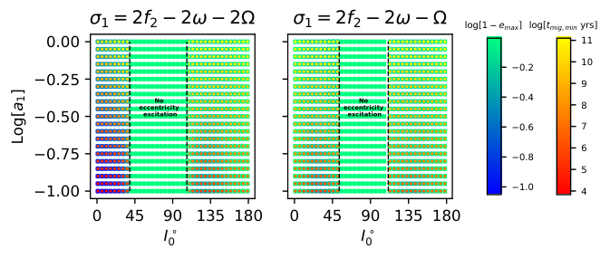

In Figure 12, the binaries are initially trapped in evection (left panel) and eviction resonances (right panel). For evection resonance, the eccentricity is excited to large values() when the initial inclination is low (). On the other hand, for eviction resonances, binary eccentricity can be excited to and above when the initial inclination is higher (). The maximum eccentricity can reach . The fastest migration timescale increases with the semi-major axis of the binary. This is consistent with Eqn. 20 which shows . The migration timescale also depends on the initial inclination. It is smallest when for evection resonances and when for eviction resonances.
Figure 13, shows results of single-averaged simulations for resonances corresponding to (left panel) and (right panel). The maximum eccentricity is largest () when the inclination is greater than for both resonances. The fastest migration timescale is small ( yrs.) at high inclinations (). Please note that the results of single-averaged simulations shown in Figures 12 and 13 are consistent with results of section II. Also, the eccentricity excitation causes the binaries to merger faster, consequently enhancing the merger rate of compact binaries in AGN disc.
IV.1.1 Location of Resonances
The location of resonances in the AGN disc is shown in Figure 14. The logarithm of the distance from the super-massive blackhole () is shown as a function of binary separation (). The minimum distance from the supermassive black-hole is shown as dashed lines and the maximum separation is shown as solid lines. The spread in is due to the dependence on the inclination of binaries. Different colors show results for different precession induced resonances. We can see that increases with the binary separation. Also, for a given binary separation, can change by an order of magnitude depending on the inclination of the binary. Generally, the resonances occur between AU. A scaling relationship can be derived using Eqn. 19:
| (29) | |||||
Please note that the factor , which depends on the initial inclination of the binary, can vary by an order of magnitude.
IV.1.2 Maximum eccentricity
The maximum eccentricity achieved by binaries trapped in resonances as a function of their initial inclination is shown in Figures 15 and 16. The initial binary separation is shown in different colors. The analytical estimates for maximum eccentricity (calculated without accounting for gravitational radiation) from Section III are shown in green. It should be noted that once a binary is trapped in a precession induced resonance, migration increases the binary eccentricity 22 2 We are only interested in parameter space where the is positive (see Figure 8). and gravitational radiation reduces the eccentricity. The maximum eccentricity is reached when the following condition is met:
| (30) |
Focusing on closely separated binaries ( AU), we can see that the simulation results are consistent with the analytical estimates when the maximum eccentricity is low (). But as the maximum eccentricity increases, gravitational radiation becomes important and suppresses the eccentricity excitation; thereby reducing the maximum eccentricity. At larger semi-major axes, both the gravitational radiation timescale () and the libration timescale () increases. Since libration timescale (and the fastest migration timescale) increases faster than the gravitational radiation timescale, they become comparable at lower eccentricities and the eccentricity excitation is suppressed. This can be seen by looking at the data points for binaries with semi-major axis 0.5 and 1 AU (colored in red and orange).
Finally, comparing different panels we can see that the eccentricity can be excited to 0.8 and above only when closely separated binaries are trapped in resonances corresponding to and (evection resonance). This is due to the fact that these resonances have the shortest libration timescales (see Figures 3 and 4). This allows them to overcome eccentricity suppression from gravitational radiation. On the other hand, libration timescale is longer for resonances corresponding to and (eviction resonance) and their ecccentricity excitation is suppressed ().
IV.1.3 Migration timescale
The fastest migration timescale which keeps the binary in resonance as a function of initial inclination is shown in Figs. 17 and 18 as filled circles. In addition, the gravitational radiation timescale is shown as solid lines. Similar to the previous plots, the semi-major axis of the binaries is shown in different colors. We can see that the migration timescale increases with the semi-major axis of the binary. The migration timescale also depends on the inclination of the binary. We can see that closely separated binaries ( AU) can migrate faster than the gravitational radiation timescale while keeping the binary in resonance. This allows the binary to merge on a faster timescale due to eccentricity excitation by the precession induced resonances. At larger binary separations ( AU), the migration timescale is comparable to the gravitational radiation timescale. Hence in this regime, precession induced resonances are not effective in reducing the merger time. It should also be noted that the AGN disk lifetime is estimated to be around years. Hence, the parameter space where the libration timescale is longer can be ignored. In our simulations, this is true for all resonances when AU.
Comparing different resonances, we can see that only closely separated binaries trapped in resonances corresponding to (evection resonance) and can significantly excite the eccentricity. Both of them have migration timescales less than the gravitational radiation timescale and the AGN disk lifetime. The libration timescales of the other two resonances is longer and comparable to gravitational radiation timescale. Hence their eccentricity excitation is suppressed.
IV.1.4 Merger time

Finally, we discuss the effects of the precession-induced resonances on the SBH mergers by characterizing the merger time of migrating binaries in these resonances. Figure 19 shows the fastest possible merger time of binaries in various precession induced resonances as a function of their semi-major axes. These results are derived from our secular simulations. We can see that the merger time increases with the semi-major axis of the binary. The merger time can be reduced by more than two orders of magnitude due to eccentricity excitation by evection resonance (, when AU). Due to longer libration timescales, binaries in resonances (Eviction resonance) and have longer merger timescales. The migration timescale is reduced by less than an order magnitude for those resonances. Binaries in experience more than order of magnitude reduction in merger time. Also, by looking at the color, we can see that the initial inclination corresponding to fastest possible merger changes with the resonant angle. In addition, the dependence of the inclination on the semi-major axis of the binary is weak. By comparing with Figures 3 and 4, we can see that the inclination shown in Figure 19 roughly corresponds to shortest libration timescale.
We conclude that precession induced resonances, particularly evection resonances, can significantly reduce the merger timescale of the binaries, and hence contribute to enhanced blackhole mergers in AGN disc.
IV.2. Resonance Capture Probability
In our simulations so far we initialized the binaries at the location of resonances. But binaries crossing a resonance will not always be captured in it. Hence, we calculate the resonance capture probability of various precession induced resonances by running an ensemble of N-body simulations. Please note that this is different from our previous paper where we used secular simulations to calculate capture probability. As N-body simulations track the dynamics in greater detail, the capture probabilities we calculate here are more accurate. For these simulations, we use the Rebound package (Rein & Liu 2012). In our code we add extra forces to simulate precession due to quadrupole moment of the circum-blackhole discs ( precession), post-Newtonian precession (1 PN order) and gravitational radiation (2.5 PN order) (e.g., Blanchet 2006; Gültekin et al. 2006).
Binary orbits are initialized with an eccentricity of and their initial inclination is sampled between 0∘ and 180∘. Initial separation of the binary from the supermassive blackhole () is chosen such that the binary starts outside the location of fixed points of the resonance (as given by Eqn. 12). The binaries are then allowed to migrate towards the supermassive blackhole on a timescale of years. The binary semi-major axis is chosen to be 0.5 AU. For a given initial inclination, we run 100 simulations in which resonant angle() is chosen uniformly between 0 and 360∘. The capture probability is calculated by counting the fraction of runs in which the binary is captured in resonance and it’s eccentricity is excited.
The results from these simulations for evection and other resonances are shown in Figures 20 and 21. For comparison we also plot the ratio of migration timescale with respect to the libration timescale in orange. We can see that the capture probability depends on the initial inclination of the binary. It is unity when the inclination of binaries captured in evection resonances is . For retrograde orbits the capture probability for evection resonances peaks at . For eviction resonance, the probability is high when . In addition, the capture probability is high () when for and for . Comparing with the orange curves, we can see that the capture probability is high when the migration timescale is slow compared to the libration timescale.
IV.3. Multiple resonance capture and resonance location
In this study so far, we have focused on circular binaries captured in one of the precession induced resonances. But it is also possible for the migrating binary to be captured in multiple resonances one after another. Focusing on planar proximity resonances first, we show in section II.4 that a migrating binary first encounters evection resonance, followed by eviction resonance and other resonances with low width. Evection resonances have large resonance width, and the binaries can hence be captured in evection resonances with high probability (see section IV.2). Once captured, the eccentricity and the inclination of the binary would increase as it migrates towards the companion. At some point the binary would encounter the bifurcation and leave the resonance (see Figure 9). The binary eccentricity and inclination are frozen at this point as it migrates further towards the companion. Since the order given in section II.4 is valid for all eccentricities, the binary would eventually encounter the eviction resonance. If captured in the eviction resonance, the binary eccentricity can be further increased at the expense of inclination. Capture into other resonances is also possible.
The likelihood of capture into multiple resonances can be determined by the product of capture probability of each capture. While an extensive study of multiple captures is not in the scope of this work, we show an example in Figure 22. We can see that the eccentricity of the binary initially captured in evection resonance increases to 0.72 and the inclination reaches . The binary then leaves the evection resonance. Till 12 million years, the binary keeps migrating inward when it encounters eviction resonance. This causes the inclination to decrease and eccentricity to increase. The resonance capture can be confirmed by looking at the bottom two panels which show the resonant angle for evection (left) and eviction (right) resonances. We can see that the resonance angle for evection resonance librates when it is in resonance at around 3 million years, and circulates at 5 million years as it is out of resonance. Similarly, at around 12 million years, the resonant angle for eviction resonance librates, but later at 14 million years it circulates.
V. Conclusions
In this paper we study the dynamics of precession induced resonances. We identify 10 such resonances in the quadrupole expansion of the Hamiltonian. Binaries trapped in 8 of these resonances can experience eccentricity excitation. We classify these resonances into planar proximity and polar proximity resonances depending on whether or not their fixed points occur in coplanar configuration. We derive analytical expressions for location of fixed points, resonance width and libration frequency for these resonances at low eccentricity. We find that many of these resonances have small resonance width and are less likely to be captured in resonances. Hence we focus on 4 resonances: (Evection resonance), (Eviction resonance), and , which have wider resonance widths and shorter libration timescale. We find that the maximum eccentricity that an initially near-circular binary can achieve depends on it’s initial inclination. The binary eccentricity can be excited to large values () when the initial inclination is less than for evection resonance, for eviction resonance, for and for resonances. In addition to eccentricity, inclination can also vary significantly. For instance, binaries captured in Evection resonance experience eccentricity and inclination increase simultaneously at low initial inclinations.
We then apply our results to binary blackholes in AGN disc. We focus on a binary composed of IMBH and a stellar mass blackhole. Using an ensemble of single-averaged simulations we list the following conclusions:
- •
Near circular binaries can be captured in precession induced resonances at a distance which increases with binary separation, mass of the companion and decreases with the mass of the central object and the quadrupole potential of the disk. It also depends on the inclination of the binary in a non-monotonic manner. The exact relationship is shown in Eqn. 29. In our fiducial simulations, the resonances occur at a distance of AU from the supermassive blackhole.
- •
The maximum eccentricity achieved by a binary trapped in a precession induced resonance depends on the inclination of the binary at capture. This is due to two reasons. Firstly, the libration timescale depends on the inclination and it is possible for the libration timescale to be comparable to the gravitational merger timescale for certain inclination range. When this happens the eccentricity excitation is suppressed. In addition, even without gravitational radiation, the maximum eccentricity a binary can attain is set by the constancy of adiabatic invariants for migrating binaries.
- •
Eccentricity excitation is possible only for binaries trapped in resonances with libration timescales shorter than the AGN disk lifetime, the gravitational merger timescale and the migration timescales in AGN disks. In our fiducial simulations, only closely separated binaries ( AU) trapped in resonances corresponding to and experience significant eccentricity excitation (). The eccentricity excitation causes the binaries to merger faster thereby enhancing the merger rate of compact binaries in AGN disc.
- •
Binaries sweeping through precession induced resonances would merge on migration timescale if the eccentricity of the binary is sufficiently excited. If the eccentricity excitation is not sufficient, the binary would be disrupted. In our fiducial simulations we find that binaries can merge 1-2 orders of magnitude faster if they migrate at the fastest rate which allows them to stay in resonance.
In addition, using an ensemble of N-body simulations, we find that the resonance capture probability is high in regions of parameter space where eccentricity can be excited to large values. We also show that migrating binaries can be captured in multiple successive precession induced resonances.
As a caveat, we use simple prescriptions for the quadrupole potential of circum-blackhole discs and migration of the binary orbits in AGN discs in this study. We also ignore binary hardening and eccentricity damping caused by the gas in the disk. Similar to our previous work (Bhaskar et al. 2022), we expect the eccentricity of the binary to be excited by resonance sweeping as long as the hardening and eccentricity damping timescales are longer than the libration timescale. Hydrodynamical simulations can be used to model the system in greater detail. For instance, using hydrodynamical simulations, Li et al. 2021 have found that the eccentricities of blackhole binaries embedded in AGN discs can be excited in regime where evection resonances are important. It remains an open question to study the eviction-like resonances using hydrodynamical simulations in the future.
References
- Antonini et al. (2014) Antonini, F., Murray, N., & Mikkola, S. 2014, ApJ, 781, 45
- Antonini et al. (2017) Antonini, F., Toonen, S., & Hamers, A. S. 2017, The Astrophysical Journal, 841, 77, aDS Bibcode: 2017ApJ…841…77A. https://ui.adsabs.harvard.edu/abs/2017ApJ...841...77A
- Askar et al. (2017) Askar, A., Szkudlarek, M., Gondek-Rosińska, D., Giersz, M., & Bulik, T. 2017, \mnras, 464, L36, _eprint: 1608.02520
- Banerjee (2017) Banerjee, S. 2017, Monthly Notices of the Royal Astronomical Society, 467, 524, aDS Bibcode: 2017MNRAS.467..524B. https://ui.adsabs.harvard.edu/abs/2017MNRAS.467..524B
- Bartos et al. (2017) Bartos, I., Kocsis, B., Haiman, Z., & Márka, S. 2017, The Astrophysical Journal, 835, 165, aDS Bibcode: 2017ApJ…835..165B. https://ui.adsabs.harvard.edu/abs/2017ApJ...835..165B
- Bavera et al. (2020) Bavera, S. S., Fragos, T., Qin, Y., et al. 2020, åp, 635, A97, _eprint: 1906.12257
- Belczynski et al. (2016) Belczynski, K., Holz, D. E., Bulik, T., & O’Shaughnessy, R. 2016, Nature, 534, 512, aDS Bibcode: 2016Natur.534..512B. https://ui.adsabs.harvard.edu/abs/2016Natur.534..512B
- Belczynski et al. (2018) Belczynski, K., Askar, A., Arca-Sedda, M., et al. 2018, Astronomy and Astrophysics, 615, A91. https://ui.adsabs.harvard.edu/abs/2018A&A...615A..91B/abstract
- Bhaskar et al. (2022) Bhaskar, H. G., Li, G., & Lin, D. N. C. 2022, The Astrophysical Journal, 934, 141, aDS Bibcode: 2022ApJ…934..141B. https://ui.adsabs.harvard.edu/abs/2022ApJ...934..141B
- Blanchet (2006) Blanchet, L. 2006, Living Reviews in Relativity, 9, 4
- Cuk & Burns (2004) Cuk, M., & Burns, J. A. 2004, \aj, 128, 2518
- Cuk et al. (2019) Cuk, M., El Moutamid, M., & Tiscareno, M. 2019, in AAS/Division of Dynamical Astronomy Meeting, Vol. 51, AAS/Division of Dynamical Astronomy Meeting, 102.05
- Di Carlo et al. (2019) Di Carlo, U. N., Giacobbo, N., Mapelli, M., et al. 2019, \mnras, 487, 2947, _eprint: 1901.00863
- Dominik et al. (2012) Dominik, M., Belczynski, K., Fryer, C., et al. 2012, The Astrophysical Journal, 759, 52, aDS Bibcode: 2012ApJ…759…52D. https://ui.adsabs.harvard.edu/abs/2012ApJ...759...52D
- Eggleton & Kiseleva-Eggleton (2001) Eggleton, P. P., & Kiseleva-Eggleton, L. 2001, \apj, 562, 1012
- Giacobbo et al. (2018) Giacobbo, N., Mapelli, M., & Spera, M. 2018, \mnras, 474, 2959, _eprint: 1711.03556
- Goldstein (1950) Goldstein, H. 1950, Classical mechanics
- Grishin et al. (2017) Grishin, E., Perets, H. B., Zenati, Y., & Michaely, E. 2017, Monthly Notices of the Royal Astronomical Society, 466, 276, aDS Bibcode: 2017MNRAS.466..276G. https://ui.adsabs.harvard.edu/abs/2017MNRAS.466..276G
- Gültekin et al. (2006) Gültekin, K., Miller, M. C., & Hamilton, D. P. 2006, ApJ, 640, 156
- Hoang et al. (2018) Hoang, B.-M., Naoz, S., Kocsis, B., Rasio, F. A., & Dosopoulou, F. 2018, The Astrophysical Journal, 856, 140, aDS Bibcode: 2018ApJ…856..140H. https://ui.adsabs.harvard.edu/abs/2018ApJ...856..140H
- Kinugawa et al. (2014) Kinugawa, T., Inayoshi, K., Hotokezaka, K., Nakauchi, D., & Nakamura, T. 2014, Monthly Notices of the Royal Astronomical Society, 442, 2963, aDS Bibcode: 2014MNRAS.442.2963K. https://ui.adsabs.harvard.edu/abs/2014MNRAS.442.2963K
- Kozai (1962) Kozai, Y. 1962, \aj, 67, 591
- Lee & Peale (2002) Lee, M. H., & Peale, S. J. 2002, The Astrophysical Journal, 567, 596. https://ui.adsabs.harvard.edu/abs/2002ApJ...567..596L
- Leigh et al. (2018) Leigh, N. W. C., Geller, A. M., McKernan, B., et al. 2018, \mnras, 474, 5672, _eprint: 1711.10494
- Li et al. (2014) Li, G., Naoz, S., Kocsis, B., & Loeb, A. 2014, ApJ, 785, 116
- Li et al. (2021) Li, Y.-P., Dempsey, A. M., Li, S., Li, H., & Li, J. 2021, ApJ, 911, 124
- Lidov (1962) Lidov, M. L. 1962, \planss, 9, 719
- Murray & Dermott (1999) Murray, C. D., & Dermott, S. F. 1999, Solar system dynamics
- Muñoz et al. (2022) Muñoz, D. J., Stone, N. C., Petrovich, C., & Rasio, F. A. 2022, Eccentric Mergers of Intermediate-Mass Black Holes from Evection Resonances in AGN Disks, arXiv, number: arXiv:2204.06002 arXiv:2204.06002 [astro-ph, physics:gr-qc], doi:10.48550/arXiv.2204.06002. http://arxiv.org/abs/2204.06002
- Naoz (2016) Naoz, S. 2016, \araa, 54, 441
- O’Leary et al. (2006) O’Leary, R. M., Rasio, F. A., Fregeau, J. M., Ivanova, N., & O’Shaughnessy, R. 2006, \apj, 637, 937
- Peters (1964) Peters, P. C. 1964, Physical Review, 136, B1224, publisher: American Physical Society. https://link.aps.org/doi/10.1103/PhysRev.136.B1224
- Rein & Liu (2012) Rein, H., & Liu, S. F. 2012, A&A, 537, A128
- Rodriguez et al. (2016) Rodriguez, C. L., Chatterjee, S., & Rasio, F. A. 2016, \prd, 93, 084029, _eprint: 1602.02444
- Samsing et al. (2014) Samsing, J., MacLeod, M., & Ramirez-Ruiz, E. 2014, The Astrophysical Journal, 784, 71, aDS Bibcode: 2014ApJ…784…71S. https://ui.adsabs.harvard.edu/abs/2014ApJ...784...71S
- Silsbee & Tremaine (2017) Silsbee, K., & Tremaine, S. 2017, \apj, 836, 39, _eprint: 1608.07642
- Spalding et al. (2016) Spalding, C., Batygin, K., & Adams, F. C. 2016, The Astrophysical Journal, 817, 18, aDS Bibcode: 2016ApJ…817…18S. https://ui.adsabs.harvard.edu/abs/2016ApJ...817...18S
- Spera et al. (2019) Spera, M., Mapelli, M., Giacobbo, N., et al. 2019, \mnras, 485, 889, _eprint: 1809.04605
- Stone et al. (2017) Stone, N. C., Metzger, B. D., & Haiman, Z. 2017, Monthly Notices of the Royal Astronomical Society, 464, 946, aDS Bibcode: 2017MNRAS.464..946S. https://ui.adsabs.harvard.edu/abs/2017MNRAS.464..946S
- Tagawa et al. (2020) Tagawa, H., Haiman, Z., & Kocsis, B. 2020, The Astrophysical Journal, 898, 25, arXiv: 1912.08218. http://arxiv.org/abs/1912.08218
- Tagawa et al. (2021) Tagawa, H., Kocsis, B., Haiman, Z., et al. 2021, The Astrophysical Journal Letters, 907, L20, arXiv:2010.10526 [astro-ph]. http://arxiv.org/abs/2010.10526
- Tian et al. (2017) Tian, Z., Wisdom, J., & Elkins-Tanton, L. 2017, Icarus, 281, 90
- Touma & Wisdom (1998) Touma, J., & Wisdom, J. 1998, The Astronomical Journal, 115, 1653. https://iopscience.iop.org/article/10.1086/300312
- Touma & Sridhar (2015) Touma, J. R., & Sridhar, S. 2015, Nature, 524, 439, aDS Bibcode: 2015Natur.524..439T. https://ui.adsabs.harvard.edu/abs/2015Natur.524..439T
- Vaillant & Correia (2022) Vaillant, T., & Correia, A. C. M. 2022, Astronomy & Astrophysics, 657, A103, arXiv: 2201.10708. http://arxiv.org/abs/2201.10708
- von Zeipel (1910) von Zeipel, H. 1910, Astronomische Nachrichten, 183, 345
- Will (2017) Will, C. M. 2017, Physical Review D, 96, 023017, aDS Bibcode: 2017PhRvD..96b3017W. https://ui.adsabs.harvard.edu/abs/2017PhRvD..96b3017W
- Xu & Lai (2016) Xu, W., & Lai, D. 2016, Monthly Notices of the Royal Astronomical Society, 459, 2925. https://academic.oup.com/mnras/article-lookup/doi/10.1093/mnras/stw890
- Yoder (1982) Yoder, C. F. 1982, Icarus, 49, 327, aDS Bibcode: 1982Icar…49..327Y. https://ui.adsabs.harvard.edu/abs/1982Icar...49..327Y
- Yokoyama (2002) Yokoyama, T. 2002, \planss, 50, 63
- Zevin et al. (2019) Zevin, M., Samsing, J., Rodriguez, C., Haster, C.-J., & Ramirez-Ruiz, E. 2019, \apj, 871, 91, _eprint: 1810.00901