Humbert Generalized Fractional Differenced ARMA Processes

Then (2.2) can be written as

The variance of the process $X_{t}$ is given by

Let $a_{n}=(mu-1)^{2n}$ and $\{b_{n}\}=\left(\frac{\Gamma(\nu+n)}{\Gamma(\nu)\Gamma(n+1)}\right)^{2}$, then using Abel’s test $\displaystyle\sum_{n=0}^{\infty}a_{n}$ converges for $0<u<\frac{2}{m}$ and using Stirling’s approximation, for large $n$, $b_{n}\simeq\frac{n^{2\nu-2}}{(\Gamma(\nu))^{2}}$, which implies that the sequence is bounded for $\nu<\frac{1}{2}$. We can write $b_{n}=\binom{\nu+n-1}{n}$ and it is known that $n\choose x$ is decreasing for $x\geq\lfloor\frac{n}{2}\rfloor$ this implies that $\{b_{n}\}$ is decreasing for $\nu\leq 1$. This indicates that the sequence is bounded and monotone for $\nu<1/2$ and the $\mathrm{Var}(X_{t})$ converges for the defined range. Similarly to prove the invertibility condition we define the process (2.2) as

where $\pi(B)=\frac{\Phi(B)}{\Theta(B)}(1-muB+B^{m})^{\nu}$ and again using the same argument discussed above the $\pi(z)$ will converge for $-\frac{1}{2}<\nu<1$ and $0<u<\frac{2}{m}$. For $u=0$ and $u=\frac{2}{m}$the variance can be defined as follows

In the above equation, the first summation is finite and the terms inside the second summation behaves like $\frac{n^{2\nu-2}}{\Gamma(\nu)^{2}}$ for large $n$ and it is bounded for $\nu<\frac{1}{2}$. Hence, the HARMA process is stationary and invertible for $\lvert\nu\rvert<1/2$ and $0\leq u\leq\frac{2}{m}$. ∎

Rewrite (2.2) as follows

where $\Psi(B)=\dfrac{\Theta(B)}{\Phi(B)}(1-muB+B^{m})^{-\nu}$. Then using the definition of spectral density of linear process, we have

where $z=e^{-\iota\omega}$ and $f_{\epsilon}(\omega)$ is spectral density of the innovation term. The spectral density of the innovation process $\epsilon_{t}$ is $\sigma^{2}/2\pi$. Then (2.5) becomes,

Here, $\left\lvert 1-mue^{-\iota\omega}+e^{-m\iota\omega}\right\rvert^{-2\nu}=(2+m^{2}u^{2}-2mu(\cos(\omega)+\cos((1-m)\omega))+2\cos(m\omega))^{-\nu}$ and the spectral density takes the following form

∎

We have the following two cases.

1. (a)

   The first term, $4\cos^{2}\left[\frac{m\omega}{2}\right]\sin^{2}\left[\frac{(m-2)\omega}{2}\right]\geq 0$ for all $m$ and $-\pi<\omega<\pi$.
   

   	$\displaystyle 4\cos^{2}\left[\frac{m\omega}{2}\right]\sin^{2}\left[\frac{(m-2)\omega}{2}\right]$	$\displaystyle=0$
   	$\displaystyle\text{ if }\cos^{2}\left(\frac{m\omega}{2}\right)$	$\displaystyle=0\text{ or }\sin^{2}\left(\frac{(m-2)\omega}{2}\right)=0\text{ or both }$
   	$\displaystyle\Rightarrow\cos\left(\frac{m\omega}{2}\right)$	$\displaystyle=0\text{ for }\omega_{1}=(4n\pm 1)\frac{\pi}{m},\text{ for all }m\in\mathbb{N}\text{ and }$
   		$\displaystyle n=0,\pm 1,\pm 2,\cdots.$

   We find the condition of singularity by solving the second term, $\left[mu-2\cos\left(\frac{m\omega}{2}\right)\cos\left(\frac{(2-m)\omega}{2}\right)\right]^{2}$ at $\omega_{1}$, which yields $u=0.$
   Also, the singular point $\omega_{1}\in(-\pi,\pi)$ for $-\frac{m\pm 1}{4}<n<\frac{m\mp 1}{4}.$
   Therefore, the type 1 HARMA$(p,\nu,u,q)$ process $\{X_{t}\}$ will have singular points for $u=0$ and $\omega_{1}=(4n\pm 1)\frac{\pi}{m}$ for all $m$ and $-\frac{m\pm 1}{4}<n<\frac{m\mp 1}{4}.$
   This proves the part $(a)$.

2. (b)

   Again the term

   $$4\cos^{2}\left(\frac{m\omega}{2}\right)\sin^{2}\left(\frac{(m-2)\omega}{2}\right)=0$$

   when

   $$\sin^{2}\left(\frac{(m-2)\omega}{2}\right)=0$$

   $$\sin\left(\frac{(m-2)\omega}{2}\right)=0\text{ for }\omega_{2}=\frac{\pm 2n\pi}{m-2}\text{ for all }m\in{\mathbb{N-}\{2\}},\\ \text{ and }n=0,\pm 1,\pm 2,\cdots.$$

   At $\omega_{2}$, the second term will become zero if and only if,

   	$\displaystyle\left[mu-\left(2\cos\left(\frac{m\omega_{2}}{2}\right)\cos\left(\frac{(2-m)\omega_{2}}{2}\right)\right)\right]^{2}$	$\displaystyle=0$
   	$\displaystyle\Rightarrow mu-2(-1)^{n}\cos\left(\pm\frac{4n\pi}{m-2}\right)$	$\displaystyle=0$
   	$\displaystyle\Rightarrow u=\frac{2(-1)^{n}}{m}\cos\left(\frac{4n\pi}{m-2}\right).$

   This proves the part $(b)$.

3. (c)

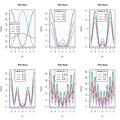
   In (2.6) let $U(\omega)=(2+m^{2}u^{2}-2mu(\cos(\omega)+\cos((1-m)\omega))+2\cos(m\omega))$. For different values of $m=1,2,3,4$ and $0\leq u<2/m$ in figure 1, we observe that the function $U(\omega)$ does not attain $0$ for $\omega\in(-\pi,\pi)$. This signifies that the spectral density defined by (2.6) has no singularity for $m=1,3,4$ and $0\leq u<2/m$. For $m=2$, the spectral density is unbounded since $U(\omega)$ takes value $0$ at $\omega=\cos^{-1}(u)$. Therefore, we conclude that for $m=2$ the singularities are at $\omega=\cos^{-1}(u)$.

∎

Now to show $b(\omega)$ is slowly varying at $\omega_{0}$, consider the case $\omega>\omega_{0}$ and for $\delta>0$ define,

and

For $\omega>\omega_{0}$ the terms $(\omega-\omega_{0})^{\delta+2\nu-1}$, $(\delta+2\nu)$ and $(2+2\cos(mw))$ are positive. It can be easily shown that

Thus in some right hand neighbourhood of $\omega_{0}$, i.e. for $\omega\to\omega_{0}^{+}$, $l^{\prime}(\omega)>0$ and $(\omega-\omega_{0})^{\delta}b(\omega)$ is increasing and similarly $(\omega-\omega_{0})^{-\delta}b(\omega)$ is decreasing when $\omega\to\omega_{0}^{+}$. Similarly, it can be easily shown that for $\omega<\omega_{0}$, $(\omega-\omega_{0})^{\delta}b(\omega)$ is decreasing and $(\omega-\omega_{0})^{-\delta}b(\omega)$ is increasing in some left hand neighbourhood of $\omega_{0}$. Thus the function is slowly varying at $\omega_{0}$.
Also, it can be easily verified that the function $b(w)$ has bounded derivative in $(0,\omega_{0}-\epsilon)\cup(\omega_{0}+\epsilon,\pi),$ hence it is of bounded variation in $(0,\omega_{0}-\epsilon)\cup(\omega_{0}+\epsilon,\pi).$

Using the above two results and the lemma 2.1 the autocorrelation function $R(h)$ of the type 1 Humbert ARMA process takes the following asymptotic form

The result (2.9) implies that the process is seasonal long memory for $0<\nu<1/2$.

References

• [1] Anh, V.V., Leonenko, N.N., Sakhno, L.M. (2004). On a class of minimum contrast estimators for fractional stochastic processes and fields. J. Statist. Plann. Inference. 123:161-185.
• [2] Anh, V.V., Knopova, V.P., Leonenko, N.N. (2004). Continuous-time stochastic processes with cyclical long-range dependence. Aust. N. Z. J. Stat.. 46(2):275–296.
• [3] Anh, V. V., Leonenko, N. N., Sakhno, L. M. (2007). Minimum contrast estimation of random processes based on information of second and third orders. J. Statist. Plann. Inference. 137(4):1302-1331.
• [4] Abramowitz, M., Stegun, I.A. (Eds.), (1992). Handbook of Mathematical Functions with Formulas, Graphs and Mathematical Tables. New York: Dover.
• [5] Baeumer, B., Meerschaert, M.M. (2010). Tempered stable Lévy motion and transient super-diffusion. J. Comput. Appl. Math. 233:2438-2448.
• [6] Baker, B. (1921). On the Relation between Pincherie’s Polynomials and the Hypergeometric Function. Proc. Edinburgh Math. Soc. 39(4):58-62.
• [7] Bartle, Robert G., Donald, R. Sherbert (2000) Introduction to real analysis. Vol. 2. New York: John Wiley.
• [8] Box, G.E.P., Jenkins, G.M. (1976). Time series analysis : forecasting and control. San Francisco: Holden-Day.
• [9] Castro, T. B., Rachinger, H. (2021). Aggregation of seasonal long-memory processes. Econom. Stat. 17:95-106.
• [10] Chung, C.-F. (1996). Estimating a generalized long memory process. J. Appl. Econometrics. 73(1):237–259.
• [11] Dissanayake, G. S., Peiris, M. S., Proietti, T. (2018). Fractionally differenced Gegenbauer processes with long memory: a review. Statist. Sci. 33:413-426.
• [12] Espejo, R. M., Leonenko, N., Ruiz-Medina, M. D. (2014). Gegenbauer random fields. Random Oper. Stoch. Equ, 22(1):1-16.
• [13] Gamelin, T. W. (2001) Complex analysis. New York: Springer.
• [14] Giraitis, L., Hidalgo, J., Robinson, P. M. (2001). Gaussian estimation of parametric spectral density with unknown pole. Ann. Statist, 29(4):987-1023.
• [15] Gould, H. W. (1965). Inverse series relations and other expansions involving Humbert polynomials. Duke Math. J. 32(4):697-711.
• [16] Grabchak, M. (2016). Tempered Stable Distributions: Stochastic Models for Multiscale Processes. New York: Springer.
• [17] Granger, C. W. J., Joyeux, R. (1980). An introduction to long-memory time series models and fractional differencing. J. Time Series Anal. 1:15-29
• [18] Gray, H.L., Zhang, N.F., Woodward, W. A.(1989). On generalized fractional processes. J. Time Series Anal. 10:233–257.
• [19] Horadam, A. F., & Pethe, S. (1981). Polynomials associated with Gegenbauer polynomials. Fibonacci Quart. 19(5): 393-398.
• [20] Horadam, A. F. (1985). Gegenbauer polynomials revisited. The Fibonacci Quart. 23(4):294-299.
• [21] Hosking, J.R.M. (1981). Fractional differencing. Biometrika. 68(1):165–176.
• [22] Humbert, P. (1920). Some extensions of Pincherle’s polynomials. Proc. Edinburgh Math. Soc. 39(1):21–24.
• [23] Ivanov, A. V., Leonenko, N., Ruiz-Medina, M. D., & Savich, I. N. (2013). Limit Theorems for weighted nonlinear transformations of Gaussian stationary processes with singular spectra. Ann. Probab., 41(2):1088-1114.
• [24] Kumar, A., Vellaisamy, P. (2014). Inverse Tempered Stable Subordinators, Statist. Probab. Lett. 103:134-141.
• [25] Milovanovic, G. V., & Djordjevic, G. B. (1987). On some properties of Humbert’s polynomials. Fibonacci Quart. 25:356-360.
• [26] Pincherle, S. (1891). Una nuova estensione delle funzioni sferiche, Memorie della Accademia Reale di Bologna (in Italian), I: 337-369.
• [27] Reisen, V. A., Rodrigues, A.L., Palma, W. (2006). Estimation of seasonal fractionally integrated processes. Comput. Statist. Data Anal. 50(2):568-582.
• [28] Rosinski, J. (2007). Tempering stable processes, Stochastic Process. Appl. 117:677–707.
• [29] Sabzikar, F., McLeod, A.I., Meerschaert, M.M. (2019). Parameter estimation for ARTFIMA time series, J. Statist. Plann. Inference. 200:129–145.
• [30] Slutsky, E. (1937). The Sommation of Random Causes as the Source of Cyclic Processes. Econometrics. 5:105-146.
• [31] Srivastava, H., & Manocha, H. (1984). Treatise on generating functions. New York: John Wiley & Sons.
• [32] Torricelli, L. Barabesi, L., Cerioli, A. (2022). Tempered positive Linnik processes and their representations. Electron. J. Stat. 16(2):6313-6347.
• [33] Wold, H. (1938). A Study in the Analysis of Stationary Time Series. Stockholm: Almgrist & Wiksell.
• [34] Yule, G.U. (1926). Why Do We Sometimes Get Nonsense-Correlations between Time Series? A Study in Sampling and the Nature of Time Series. J. R. Stat. Soc. 89:1-64.
• [35] Zheng, M., Karniadakis, G.E. (2015). Numerical Methods for SPDEs with Tempered Stable Processes. SIAM J. Sci. Comput. 37(3).