An entropic uncertainty principle for mixed states

Introduction. Uncertainty relations express the limits imposed by quantum mechanics on our ability to either prepare a state with given properties, or measure the properties of a state to a given precision mur; entromur; busch; blw. The study of uncertainty inequalities dates back to some of the most famous works of the early days of quantum theory heisenberg; schrodinger; weyl1928; robertson; kennard and has since then stayed a topic of ongoing research hirschmann; alberto; alberto2; colesfurrer; meandist; review1; entro9; gao. Besides being an attractive rabbit hole by its own rudnicki2014strong; abbot; carlos; entroaddi; konrad; ourentro; rastegin; zozor; xie; wang, having the right uncertainty relation at hand often proved to be a powerful tool berta; schneeloch; ballesterwehner; spinsqueezing; riccardi2022entanglement; ana, e.g. to build a worst-case model. For example, uncertainty relations commonly serve as an easy-to-establish estimate that allows determining, from measured data, properties like the presence of entanglement guhne; guhne2; hofmann; variances; bergh; brunner, or the amount of extractable secure randomness berta; tomamichel; masini; ddorf; di1; di2.

In quantum information theory, uncertainty is typically quantified in terms of entropies. The prototype uncertainty relation of this type is due to an idea of Deutsch deutsch and a conjecture by Kraus kraus1987complementary proven by Maassen and Uffink muf: Let $X$ and $Y$ denote two projective measurements, then the possible values of the Shannon entropies of their measurement outcomes, $H(X)$ and $H(Y)$, (measured on copies of a state $\rho$) are constraint by

Here $c_{\text{\tiny KMU}}$ (see eq. (8)) is a non-negative constant that depends on the overlap between the measurement bases of $X$ and $Y$, and $S(\rho)$ is the von Neumann entropy of $\rho$.

In this note, we establish a generalization of (1) to a family of entropic uncertainty relations of the form:

with parameters $\mu,\lambda,\alpha\in[0,1]$. More precisely, we are interested in finding a constant $c_{XY}(\alpha,\lambda,\mu)$ such that (2) holds for all states $\rho$. Our main result Thm. 1 provides this constant by drawing a connection to the norm of the doubly stochastic map that links the probability distributions in the $X$ and the $Y$ bases.

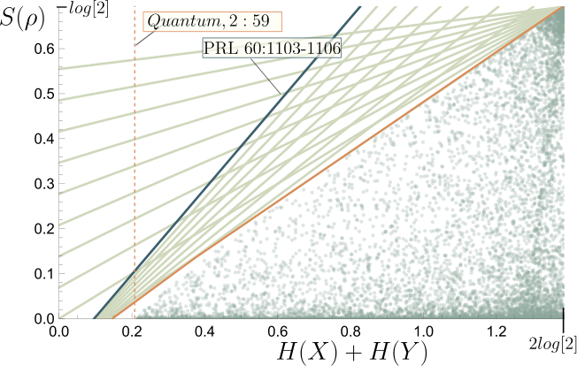
The von Neumann entropy term on the r.h.s. of (1) was not present in the original formulation of this inequality. It was however noted by Frank & Lieb hanstalk; frank and Berta et al. berta, that it can be added without changing the constant $c_{\text{\tiny KMU}}$. An interesting consequence, which is often overlooked, is that a state that minimizes the gap of this inequality will not necessarily be pure. We extend this by including a weight $\alpha$ for the entropy term on the r.h.s. of (2). The factor $\alpha$ sets the degree of mixedness that a state that minimizes the gap has. This goes from pure states that saturate (2) for $\alpha=0$ (see ourentro) to the maximally mixed state that saturates (2) for $\alpha=2$ and $\mu+\lambda=1$ with $c_{XY}=0$. By this, we get a natural notion of a family of most certain (i.e. minimally uncertain) mixed states for measurements $X$ and $Y$.

An uncertainty relation like (2) can also be used to estimate the von Neumann entropy of an unknown state with given values of $H(X)$ and $H(Y)$, obtained e.g. from measurement data. This has various practical applications. For example, consider the scenario in which a local system $A$, with a reduced state $\rho_{A}$, has interacted with an uncharacterized environment $E$. Here (2) becomes handy for estimating correlations, since $S(\rho_{A})$ describes the corresponding entanglement entropy. Building on this perspective, we demonstrate how to use our results for bounding the securely extractable randomness of a source independent quantum random number generator, for attesting entanglement between two trusted parties, and between two trusted parties and an uncharacterized environment.

Parameterized uncertainty relations. Including weights, like $\alpha,\lambda,\mu$ in (2), is a natural way of strengthening an existing relation. This has to be contrasted with many proposed improvements of the Maassen and Uffink relation that merely add more and more $\rho$-dependent terms to the r.h.s. of (1).

One typical primordial question, preceding the use of an uncertainty relation, is to characterize the set of possible triples $\Omega_{XY}:=\{(H(X),H(Y),S(\rho))\}_{\rho}$ that could be attained by a not further specified state $\rho$. Our result (2) directly serves this purpose by giving bounds on arbitrary linear combination of $H(X)$, $H(Y)$, and $S(\rho)$. Given a valid value of $c_{XY}$ for all parameters $(\alpha,\mu,\lambda)$ allows for reconstructing a convex outer approximation to $\Omega_{XY}$ by performing a Legendre transformation amu of $c_{XY}$ with respect to $\alpha,\lambda,\mu$.

Another typical use of an uncertainty relation is to bound the value of one quantity given access to the others. The estimation of $S(\rho)$, mentioned above, is an example of this. Here a given value of $c_{XY}$ for a whole parameter range directly pays off when we use (2) to obtain the estimate

In general, this gives stronger estimates than (1), which corresponds to evaluating the minimization above on the single point $\lambda=\mu=1$.

The main result of this work is the following theorem, which provides a closed form for $c_{XY}$ in terms of operator norms:

The norm appearing in the theorem is defined by

where $\norm{\cdot}_{p}$ denotes the usual $p$-norm.

Plugging eq. (4) in eq. (2), we find

How to evaluate the norm. In principle, the operator norm in the bound provided by (6) can be computed numerically with arbitrary precision. However, for large system sizes, this may turn out to be challenging in practise. Therefore, we provide some analytical results and a conjecture that may drastically simplify this computation. From now on, we specialize to rank-1 projective measurements; in this case, we can associate orthonormal bases to $X$ and $Y$. We denote by $d$ the number of projectors, i.e. the dimension of the Hilbert space.

When the bases of $X$ and $Y$ are mutually unbiased (MUB), $C^{(2)}$ has all entries equal to $1/d$. Its norm is (Lemma 3 in additional)

One can show (Lemma 7 in additional), that this equation in fact holds for any matrix $C^{(2)}$ as long as $\mu+\lambda\leq 1$. In the limit $\mu=\lambda\rightarrow 1$, we recover the well-known result of Kraus, Maassen and Uffink (KMU) kraus1987complementary; muf,

What we have learned about these norms is summarized in Fig. 2.

We observe an interesting fact: the norm of $C^{(2)}$ seems to follow the MUB result beyond $\mu=1/2$, up to a critical value $\mu_{*}$. One can check that a similar behaviour is also found in higher dimensions, and for $\mu\neq\lambda$. This leads us to formulate the following conjecture.

Comparison to existing uncertainty relations. In this section, we compare (6) with two other known EUR: that of berta, which we denote BCCRR,

and the inequality RPZ₂ from rudnicki2014strong,

Here, following rudnicki2014strong, $c_{1}$ and $c_{2}$ denote the first and second largest elements of $C^{(2)}$, and $C\equiv(1+\sqrt{c_{1}})/2$.

To compare with these inequalities, which give equal weights to $H(X)$ and $H(Y)$, we set $\mu=\lambda$. Using conjecture 1 and setting $\mu=\mu_{*}$ as in eq. (10), we find

The entropy term in eq. (13) is always larger than in both BCCRR and RPZ₂. Therefore, in our comparison, we consider only the second, state-independent, term.

We first consider $d=2$. In this case, the most general $C^{(2)}$ matrix is given by

where $\theta=0$ corresponds to $X=Y$, and $\theta=\pi/4$ to the MUB case.

The bounds provided by BCCRR, RPZ₂, and eq. (13) are compared in Fig. 3. The bounds are equivalent for $\theta=0$ and $\theta=\pi/4$, while in between our bound is stronger.

For $d>2$, the matrices $C^{(2)}$ have too many parameters, and we cannot scan them all, as we did in Fig. 3. Instead, we compare our bound, eq. (13), to BCCRR and RPZ₂ for some random $C^{(2)}$, generated by setting $C^{(2)}_{ij}=\absolutevalue{U_{ij}}^{2}$, where $U$ is a Haar random unitary. In Fig. 4, we plot the percentage of $C^{(2)}$ for which our bound is better than BCCRR or RPZ₂ as a function of $d$.

As expected, for $d=2$, our bound is always at least as good as both BCCRR and RPZ₂. The percentage of $C^{(2)}$ for which our bound is better decreases for $d=3,4$, but then starts increasing. For $d\gg 1$, our bound is equivalent or better with probability that approaches 1.

Practical applications. From the comparison above, we know that eq. (6), for $\mu=\lambda$, provides stronger constraints compared to other EUR for many observables $X$ and $Y$ (eq. (13)). Therefore, it can be useful in all applications of other EUR. However, imposing $\mu=\lambda$ we loose part of the power of eq. (6), i.e. that of giving different weights to $H(X)$ and $H(Y)$. This is often beneficial in practical applications, as we show in three examples: bounding extractable randomness, entanglement detection, and bounding entanglement with an eavesdropper.

Bounding extractable randomness. Quantum random number generators will likely be one of the first competing market-ready quantum devices. However, proving their security without imposing too strong assumptions is still under development. A promising class of protocols are source-independent random number generators. Their basic security mechanism can be traced back to the use of the uncertainty relation (1). Our results can be directly used to get stronger bounds on the extractable randomness.

In a basic protocol cao, we are provided with a state $\rho$, emitted by an untrusted source, from which we want to extract random numbers. We are allowed to perform measurements $X$ and $Y$. By convention, the $X$ measurement will be used for generating a secret number. The entropy $H(Y)$ of the other measurement, in this context usually referred to as phase-error rate, will be used to certify properties of $\rho$. We consider fully quantum attacks, modeled by granting an adversary $E$ full access to the purification of $\rho$.

It was shown in rotem; rennerphd that the single-shot quantity that has to be bounded for estimating the rate of securely extractable randomness (both asymptotically and finite) is given by the conditional entropy $H(X|E)$, which in our case can equivalently tan be computed by $H(X)-S(\rho)$. Using (6), we can bound this expression as

The main advantage of using eq. (6) is that we can optimize over $\mu$ and $\lambda$ to obtain improved bounds compared to other symmetric EUR. The optimal value can be found by numerically evaluating the norm.

Using conjecture 1, we can avoid numerics and get an analytical bound. Let $\Delta_{X}\equiv\log{d}-H(X)$, $\Delta_{Y}\equiv\log{d}-H(Y)$, then one can show that, as long as (9) is satisfied, the optimal bound is additional

where $\gamma\equiv\sqrt{\Delta_{X}/\Delta_{Y}}$. Notice that wlog we can assume that $\gamma\leq 1$ (swap $X$ and $Y$ if this is not the case).

Entanglement detection. Consider now a bipartite state $\rho_{AB}$, shared between two parties, $A$ and $B$, that can perform local measurements, $X_{AB}=X_{A}\otimes X_{B}$, $Y_{AB}=Y_{A}\otimes Y_{B}$, and exchange classical information. To use eq. (6) for detecting entanglement, we follow riccardi2022entanglement; one can show that $\rho_{AB}$ is entangled if additional

Here $S_{max}=\max(S(\rho_{A}),S(\rho_{B}))$.

We can use conjecture 1 to find a condition that is easier to treat analytically. Let $\sigma_{2}=\max(\sigma_{2,A},\sigma_{2,B})$, where $\sigma_{2,A}$ and $\sigma_{2,B}$ are the second largest singular values of $C^{(2)}_{A}$ and $C^{(2)}_{B}$. Then, as long as $\mu,\lambda$ obey eq. (9), we find that $\rho_{AB}$ is entangled if

Here, $\Delta_{X}\equiv\log{d}-H(X_{AB})$, $\Delta_{Y}\equiv\log{d}-H(Y_{AB})$, and $d=d_{A}d_{B}$ is the total size of the Hilbert space. Since both $\Delta_{X}$ and $\Delta_{Y}$ are non-negative, the best we can do is to take $\mu$ and $\lambda$ as big as possible. However, the constraints (9) prevents us from increasing $\mu$ and $\lambda$ independently. The optimal value of $(\mu,\lambda)$ for given $\Delta_{X,Y}$ is additional

if $\sigma_{2}\leq\gamma\leq 1/\sigma_{2}$. When $\gamma<\sigma_{2}$, the optimal choice is $(\mu,\lambda)=(1,0)$, and, when $\gamma>1/\sigma_{2}$, it is $(\mu,\lambda)=(0,1)$. In the original notation, in terms of $H(X)$ and $H(Y)$, we find that, for $\sigma_{2}\leq\gamma\leq 1/\sigma_{2}$, $\rho_{AB}$ is entangled if

We conclude that the freedom of keeping $\mu\neq\lambda$ generally helps. However, notice that for MUB $\sigma_{2}=0$, and we can take $\mu=\lambda=1$.

As an example, we consider Werner states werner1989quantum

where $V=\sum_{ij}|ij\rangle\langle ji|$ is the swap operator, and $\Phi\in[-1,1]$. These states are entangled for $\Phi<0$. We consider Werner states of two qubits, $d_{A}=d_{B}=2$, take $X_{A,B}$ in the computational basis, and $Y_{A}$,$Y_{B}$ in bases rotated by angles $\theta_{A}$, $\theta_{B}$. In Fig. 5, we plot for which values of $(\theta_{A},\theta_{B})$ eq. (20) can detect entangled Werner states for various values of $\Phi<0$.

The set of measurements able to detect entangled Werner states shrinks as we increase $\Phi$. Measurements in MUB (top-right corner) are the most powerful for detecting entanglement.

Bound on entropy. Consider the same setup as in the entanglement detection example; A and B are now interested in quantifying how much entanglement they might share with an eavesdropper, E. Let $\rho_{ABE}$ be the joint state of A, B, and E; in the worst case, this state is pure, and $S(\rho_{E})=S(\rho_{AB})$. A direct application of eq. (6) gives the following bound:

To obtain an analytic result, we can again use our conjecture, and proceed similarly to what we did above for entanglement detection. As long as $\sigma_{2}\leq\gamma\leq 1/\sigma_{2}$, we find that the optimal choices for $\mu$ and $\lambda$ are again given by (19), where $\sigma_{2}$ is now the second largest singular value of $C^{(2)}_{AB}$. We arrive at the following improved bound for $S(E)$,

Notice that, for MUB, we find again that the best we can do is to set $\mu=\lambda=1$.

Conclusions. In this article, we have introduced a new class of EUR, eq. (6), which allows giving different weights to $H(X)$, $H(Y)$, and $S(\rho)$. We have shown that these EUR often provide better bounds than other EUR known in the literature. Moreover, we have shown in three examples that the freedom of giving different weights can be helpful in practical applications. Eq. (6) is expressed in terms of norms, which are difficult to estimate numerically. We have explored properties of these norms, and formulated a conjecture that, if correct, leads to an analytic result valid for most of the parameter space. In particular, we have obtained eq. (13), that provides a simple alternative to Maassen-Uffink, where $\log{c_{MU}}$ is replaced by $(1-\sigma_{2})\log d$.

There are several directions in which this work could be extended. Clearly, it would be nice to prove conjecture 1. Also, using conjecture 1, we can analytically study eq. (6) for values of $(\mu,\lambda)$ satisfying eq. (9). Close to $\mu=\lambda=1$, the KMU result applies. It remains to explore eq. (6) for intermediate values of $(\mu,\lambda)$. Finally, for applications to QKD, it would be interesting to extend eq. (6) to Renyi and conditional entropies.