Benchmarking Robustness of 3D Object Detection to Common Corruptions
in Autonomous Driving
Abstract
3D object detection is an important task in autonomous driving to perceive the surroundings. Despite the excellent performance, the existing 3D detectors lack the robustness to real-world corruptions caused by adverse weathers, sensor noises, etc., provoking concerns about the safety and reliability of autonomous driving systems. To comprehensively and rigorously benchmark the corruption robustness of 3D detectors, in this paper we design 27 types of common corruptions for both LiDAR and camera inputs considering real-world driving scenarios. By synthesizing these corruptions on public datasets, we establish three corruption robustness benchmarks—KITTI-C, nuScenes-C, and Waymo-C. Then, we conduct large-scale experiments on 24 diverse 3D object detection models to evaluate their corruption robustness. Based on the evaluation results, we draw several important findings, including: 1) motion-level corruptions are the most threatening ones that lead to significant performance drop of all models; 2) LiDAR-camera fusion models demonstrate better robustness; 3) camera-only models are extremely vulnerable to image corruptions, showing the indispensability of LiDAR point clouds. We release the benchmarks and codes at https://github.com/kkkcx/3D_Corruptions_AD. We hope that our benchmarks and findings can provide insights for future research on developing robust 3D object detection models.
1 Introduction
As a fundamental task in autonomous driving, 3D object detection aims to identify objects of interest (e.g., vehicles, pedestrians, or cyclists) in the surrounding environment by predicting their categories and the corresponding 3D bounding boxes. LiDAR and camera are two important types of sensors for 3D object detection, where the former provides the depth information of road objects as sparse point clouds, while the latter captures abundant semantic information of the scene as color images. Based on the complementary nature of the two modalities, 3D object detection models can be categorized into LiDAR-only zhou2018voxelnet; lang2019pointpillars; shi2019pointrcnn; yan2018second; shi2020pv, camera-only mousavian20173d; wang2019pseudo; wang2021fcos3d; wang2022detr3d, and LiDAR-camera fusion chen2017multi; ku2018joint; vora2020pointpainting; liang2018deep models. Since autonomous driving is safety-critical, it is of paramount importance to assess the robustness of 3D object detectors under diverse circumstances before deployed.
Although the recent progress of 3D object detection has led to significant improvements in typical benchmarks (e.g., KITTI geiger2012we, nuScenes caesar2020nuscenes, and Waymo sun2020scalability), the existing models based on data-driven deep learning approaches often generalize poorly to the corrupted data caused by, e.g., adverse weathers kilic2021lidar; hahner2021fog; hahner2022lidar, sensor noises carballo2020libre; ren2022benchmarking; hendrycks2018benchmarking, and uncommon objects chan2021segmentmeifyoucan; li2022coda, posing a formidable obstacle to safe and reliable autonomous driving safecar. To perform robustness evaluation, recent works construct new datasets of road anomalies li2022coda; chan2021segmentmeifyoucan; pinggera2016lost; pmlr-v162-hendrycks22a or under extreme weather conditions bijelic2020seeing; pitropov2021canadian; diaz2022ithaca365. Nevertheless, they are usually of small sizes due to the high data collection costs and the rareness of corner cases or adverse weathers. Other works synthesize common corruptions on clean datasets to benchmark robustness on image classification hendrycks2018benchmarking and point cloud recognition ren2022benchmarking; sun2022benchmarking, but they only consider several simple corruptions, which could be insufficient and unrealistic for 3D object detection. Therefore, it remains challenging to comprehensively characterize different corruptions considering diverse driving scenarios and fairly evaluate corruption robustness of existing models within a unified framework.

In this paper, we systematically design 27 types of common corruptions in 3D object detection for both LiDAR and camera sensors to comprehensively and rigorously evaluate the corruption robustness of current 3D object detectors. The corruptions are grouped into weather, sensor, motion, object, and alignment levels, covering the majority of real-world corruption cases, as demonstrated in Fig. 1. Most of them are specifically designed for autonomous driving (e.g., motion-level ones), which have not been explored before. Following hendrycks2018benchmarking, every corruption has five severities, leading to a total number of 135 distinct corruptions. By applying them to typical autonomous driving datasets—KITTI geiger2012we, nuScenes caesar2020nuscenes, and Waymo sun2020scalability, we establish three corruption robustness benchmarks—KITTI-C, nuScenes-C, and Waymo-C. We hope that these large-scale corrupted datasets can serve as general datasets for fairly and comprehensively benchmarking corruption robustness of 3D object detection models and facilitating future research.
We conduct large-scale experiments to compare the corruption robustness of existing 3D object detection models. Specifically, we evaluate 11 models on KITTI-C, 10 models on nuScenes-C, and 3 models on Waymo-C. The models are of great variety with different input modalities, representation methods, and detection heads. Based on the evaluation results, we find that: 1) the corruption robustness of 3D object detectors is highly correlated with their clean accuracy; 2) motion-level corruptions impair the model performance most, while being rarely explored before; 3) LiDAR-camera fusion models are more resistant to corruptions, but there is a trade-off between robustness under image corruptions and point cloud corruptions of fusion models. More discussions are provided in Sec. 6. Moreover, we study data augmentation strategies choi2021part; zhang2022pointcutmix; yun2019cutmix as potential solutions to improve corruption robustness, but find that they provide a little robustness gain, leaving robustness enhancement of 3D object detection an open problem for future research.
2 Related Work
2.1 3D Object Detection
Based on the input modality, we categorize 3D object detection models into LiDAR-only, camera-only, and LiDAR-camera fusion models.
LiDAR-only models: LiDAR point clouds are sparse, irregular, and unordered by nature. To learn useful representations, voxel-based methods project point clouds to compact grids. Typically, VoxelNet zhou2018voxelnet rasterizes point clouds into voxels, which are processed by PointNets qi2017pointnet and 3D CNNs. To speed up, SECOND yan2018second introduces sparse 3D convolutions and PointPillars lang2019pointpillars elongates voxels into pillars. Other works exploit information of object parts shi2020points or shape zhu2020ssn to improve the performance. On the other hand, point-based methods take raw point clouds as inputs and make predictions on each point. PointRCNN shi2019pointrcnn proposes a two-stage framework that first generates 3D proposals and then refines the proposals in the canonical coordinates. 3DSSD yang20203dssd is a lightweight one-stage detector with a fusion sampling strategy. To have the best of both worlds, point-voxel-based methods are then explored. PV-RCNN shi2020pv integrates 3D voxel CNN and PointNet-based set abstraction to efficiently create high-quality proposals.
Camera-only models: 3D object detection based on images is challenging due to the lack of depth information, but attracts extensive attention considering the advantage of low cost. The most straightforward approach is to take monocular detection methods liu2020smoke; wang2021fcos3d; mousavian20173d; wang2019pseudo; chen2016monocular and apply post-processing across cameras. For example, Mono3D chen2016monocular generates 3D object proposals scored by semantic features. SMOKE liu2020smoke combines a single keypoint estimation with regressed 3D variables. To address the limitation of post-processing in monocular methods, multi-view methods fuse information from all cameras in the intermediate layers. DETR3D wang2022detr3d adopts a transformer-based detector carion2020end that fetches the image features by projecting object queries onto images. BEVFormer li2022bevformer exploits spatial-temporal information from multi-view images based on BEV queries.
LiDAR-camera fusion models: To leverage the complementary information from LiDAR and camera inputs, fusion methods are also extensively studied. Following liu2022bevfusion, we classify the newly developed methods into point-level, proposal-level, and unified representation fusion methods. Point-level methods augment LiDAR point clouds with semantic image features and then apply existing LiDAR-only models for 3D detection, including PointPainting vora2020pointpainting, EPNet huang2020epnet, PointAugmenting wang2021pointaugmenting, Focals Conv chen2022focal, etc. Proposal-level fusion methods chen2017multi; qi2018frustum generate 3D object proposals and integrate image features into these proposals. FUTR3D chen2022futr3d and TransFusion bai2022transfusion employ a query-based transformer decoder, which fuses image features with object queries. Moreover, BEVFusion liu2022bevfusion unifies the image feature and point cloud feature in a BEV representation space, which stands out as a new fusion strategy.
2.2 Robustness Benchmarks
It is well-known that deep learning models lack the robustness to adversarial examples szegedy2013intriguing; goodfellow2014explaining, common corruptions hendrycks2018benchmarking, and other kinds of distribution shifts hendrycks2021many; geirhos2018generalisation; geirhos2018imagenet. In autonomous driving, many works collect new datasets to evaluate model robustness under different conditions. For example, the Seeing Through Fog (STF) bijelic2020seeing, Canadian Adverse Driving Conditions (CADC) pitropov2021canadian, and Ithaca365 diaz2022ithaca365 datasets are collected in adverse weathers; and others gather road anomalies of 2D images li2022coda; chan2021segmentmeifyoucan; pinggera2016lost; pmlr-v162-hendrycks22a. Despite the efforts, these datasets only cover limited scenarios due to the high collection costs of rare data. Moreover, as mainly used for evaluation, these datasets have a big domain gap from the large-scale training datasets since they were collected in different cities with varying vehicles and sensors, making it hard for us to examine the effects of different factors (e.g., weather vs. city) on model robustness.
One promising direction is to synthesize real-world corruptions on clean datasets to benchmark model robustness. For example, ImageNet-C hendrycks2018benchmarking is first introduced in image classification with 15 corruption types, ranging from noise, blur, weather to digital corruptions. The similar methodology is further applied to 2D object detection michaelis2019benchmarking and point cloud recognition sun2022benchmarking; ren2022benchmarking. However, many of these studied corruptions are hypothetical and thus unrealistic in the scenario of autonomous driving. It is still challenging to build a comprehensive benchmark for robustness evaluation of 3D object detection considering diverse real-world driving cases. We notice that two concurrent works li2022common; yu2022benchmarking to ours also study robustness of 3D object detection in autonomous driving. However, they mainly consider specific kinds of 3D detection models (i.e., LiDAR-only models in li2022common and fusion models in yu2022benchmarking) and include limited types of corruptions with less evaluations, as compared in Appendix A.2.
3 Corruptions in 3D Object Detection
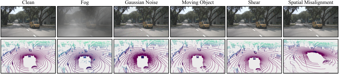
Real-world corruptions arise from diverse scenarios in autonomous driving, based on which we systematically categorize the corruptions into weather, sensor, motion, object, and alignment levels. We identify common corruption types for each level considering real-world driving scenarios, resulting in 27 distinct corruptions in total, as shown in Fig. 1. Among them, some corruptions are applied to both modalities simultaneously, such as weather-level ones, while the others are designed for a single modality, such as sensor-level ones. We visualize a subset of corruptions in Fig. 2.
Weather-level corruptions: Weather change is usually encountered in autonomous driving, which can dramatically disrupt both LiDAR and camera inputs. For example, fog reduces the visibility of objects in images and causes scattered points due to attenuation and backscattering bijelic2020seeing; hahner2021fog; zang2019impact. Consequently, 3D detectors trained on data collected in normal weather tend to perform poorly under adverse weathers bijelic2020seeing. To study the robustness under weather changes, we consider 4 weather-level corruptions: Snow, Rain, Fog, and Strong Sunlight, as they are more common bijelic2020seeing; pitropov2021canadian; diaz2022ithaca365. For LiDAR, we adopt physically based methods kilic2021lidar; hahner2022lidar; hahner2021fog to simulate the effects of rain, snow, and fog on point clouds from normal weather. We simulate the effect of strong sunlight by applying strong Gaussian noises to points along the sun direction carballo2020libre. For camera, we apply image augmentations hendrycks2018benchmarking to simulate visually realistic weathers.
Sensor-level corruptions: The sensors, when affected by numerous internal or external factors (e.g., sensor vibration schlager2022automotive, lighting conditions li2022bevformer; hendrycks2018benchmarking and reflective materials), can induce various kinds of corruptions to the captured data. Based on prior discussions on sensor noises carballo2020libre; ren2022benchmarking; berger2014state; hendrycks2018benchmarking, we design 10 practical sensor-level corruptions—7 for point clouds and 3 for images. The point cloud corruptions are: Density Decrease, Cutout, LiDAR Crosstalk, FOV Lost, Gaussian Noise, Uniform Noise, and Impulse Noise. Density decrease simulates missing points commonly observed in typical datasets geiger2012we. Cutout occurs when laser pulses have no echo in a local region (e.g., puddle) and is simulated by dropping points in a randomly selected area. LiDAR crosstalk brinon2021methodology happens when multiple LiDARs operate at close range, which is simulated by applying strong Gaussian noises to a small subset of points. FOV lost simulates a limited field-of-view of LiDAR caused by occlusion. Moreover, due to the ranging inaccuracy of LiDAR, we consider 3 noise corruptions that apply Gaussian, uniform, and impulse noises to point coordinates, respectively. The 3 image corruptions include: Gaussian Noise, Uniform Noise, and Impulse Noise to simulate the visual noise patterns due to low-lighting conditions or defects of camera hendrycks2018benchmarking. Although we design sensor-level corruptions for LiDAR and camera separately, they can occur for both sensors at the same time, affecting LiDAR-camera fusion models further.
Motion-level corruptions: An autonomous vehicle will encounter several types of corruptions during driving. In this paper, we introduce 3 motion-level corruptions: Motion Compensation, Moving Object, and Motion Blur, which are practical in the real world and studied for the first time. Vehicle ego-motion induces distortions to point clouds since the points in a frame are not obtained in the same coordinate system zhang2014loam. To obtain accurate point clouds, motion compensation is typically used with the aid of the localization information geiger2012we; caesar2020nuscenes. However, this process can introduce noises, which we call motion compensation corruption, simulated by adding small Gaussian noises to the rotation and translation matrices of the vehicle’s ego pose. The moving object corruption denotes the case that an object is moving rapidly in the scene. It can cause shifting points within the object’s 3D bounding box wen2019gnss and blur the image patch of the object. The last corruption is motion blur on camera images, which is caused by driving too fast.
Object-level corruptions: Objects in the real world always come in a variety of shapes and materials chan2021segmentmeifyoucan; li2022coda, making it challenging to correctly recognize them. The viewing direction can also lead to wrong recognition of objects dong2022viewfool. Based on this, we introduce 8 object-level corruptions: Local Density Decrease, Local Cutout, Local Gaussian Noise, Local Uniform Noise, Local Impluse Noise, Shear, Scale, and Rotation. The first five corruptions are only applied to LiDAR point clouds to simulate the distortions caused by different object materials or occlusion. As their names indicate, these corruptions only make changes to local sets of points within the objects’ 3D bounding boxes. The last three corruptions simulate shape deformation of objects, and Rotation can also simulate different view directions of objects. They can affect both LiDAR and camera inputs. To make consistent distortions to two modalities, we apply the same transformation of shear, scale, or rotation to both points and image patches belonging to the objects in the scene.
Alignment-level corruptions: It was typically assumed that LiDAR and camera inputs are well aligned before feeding to the fusion models. However, this assumption can be invalid during long-time driving, e.g., the collection of the ONCE dataset mao2021one needs re-calibration almost every day to avoid misalignment between different sensors. In practice, an autonomous vehicle can encounter Spatial Misalignment and Temporal Misalignment yu2022benchmarking. Spatial misalignment can be caused by sensor vibration due to bumps of the vehicle. We simulate it by adding random noises to the calibration matrices. Temporal misalignment happens when the data is stuck or delayed for a sensor. We keep the input of one modality the same as that at the previous timestamp to simulate temporal misalignment between the two modalities.
Discussion about the gap between synthetic and real-world corruptions. Real-world corruptions can come from multiple and diverse sources. For example, an autonomous vehicle can encounter adverse weather and uncommon objects at the same time, leading to much more complicated corruptions. Although it is impossible to enumerate all real-world corruptions, we systematically design 27 corruption types grouped into five levels, which can serve as a practical testbed to perform controllable robustness evaluation. Especially, for weather-level corruptions, we adopt the state-of-the-art methods for simulation, which are shown to approximate real data well hahner2022lidar; hahner2021fog. Although there inevitably exists a gap, we validate that the model performance on synthetic weathers are consistent with that on real data under adverse weathers. More discussions are provided in Appendix A.4.
4 Corruption Robustness Benchmarks
| Model | Modality | Representation | Detection |
|---|---|---|---|
| SECOND yan2018second | LiDAR-only | voxel-based | one-stage |
| PointPillars lang2019pointpillars | LiDAR-only | voxel-based | one-stage |
| PointRCNN shi2019pointrcnn | LiDAR-only | point-based | two-stage |
| Part- shi2020points | LiDAR-only | voxel-based | two-stage |
| PV-RCNN shi2020pv | LiDAR-only | point-voxel-based | two-stage |
| 3DSSD yang20203dssd | LiDAR-only | point-based | one-stage |
| SMOKE liu2020smoke | camera-only | monocular | one-stage |
| PGD wang2022probabilistic | camera-only | monocular | one-stage |
| ImVoxelNet rukhovich2022imvoxelnet | camera-only | monocular | one-stage |
| EPNet huang2020epnet | fusion | point-level | two-stage |
| Focals Conv chen2022focal | fusion | point-level | two-stage |
| Model | Modality | Representation | Detection |
|---|---|---|---|
| PointPillars lang2019pointpillars | LiDAR-only | voxel-based | one-stage |
| SSN zhu2020ssn | LiDAR-only | voxel-based | one-stage |
| CenterPoint yin2021center | LiDAR-only | voxel-based | two-stage |
| FCOS3D wang2021fcos3d | camera-only | monocular | one-stage |
| PGD wang2022probabilistic | camera-only | monocular | one-stage |
| DETR3D wang2022detr3d | camera-only | multi-view | query-based |
| BEVFormer li2022bevformer | camera-only | multi-view | query-based |
| FUTR3D chen2022futr3d | fusion | proposal-level | query-based |
| TransFusion bai2022transfusion | fusion | proposal-level | query-based |
| BEVFusion liu2022bevfusion | fusion | unified | query-based |
To comprehensively evaluate the corruption robustness of 3D object detection models, we establish three corruption robustness benchmarks based on the most widely used datasets in autonomous driving—KITTI geiger2012we, nuScenes caesar2020nuscenes, and Waymo sun2020scalability. We apply the aforementioned corruptions to the validation sets of these datasets and obtain KITTI-C, nuScenes-C, and Waymo-C, respectively. Note that although several corruptions naturally appear in few samples of the datasets, we still apply the synthetic corruptions to all data to fairly compare model robustness under different corruptions and reduce the efforts of filtering data. Besides, we build a unified toolkit comprising of all corruptions, that can be used for other datasets as well. Below we introduce the dataset details, evaluation metrics, and evaluated models of the three benchmarks, respectively.
4.1 KITTI-C
The KITTI dataset geiger2012we contains 3712 training, 3769 validation, and 7518 test samples. As we do not have access to the test set, KITTI-C is constructed upon the validation set. Among the corruptions, we do not include FOV Lost, Motion Compensation and Temporal Misalignment since: 1) 3D object detection models usually take front-view point clouds of FOV as inputs since the KITTI dataset only provides box annotations in front of the vehicle; 2) the localization and timestamp information of each frame is not provided in the dataset. Therefore, there are 24 corruptions in KITTI-C with 5 severities for each following hendrycks2018benchmarking.
The standard evaluation is performed on Car, Pedestrian and Cyclist categories at Easy, Moderate and Hard levels of difficulty. The evaluation metric is the Average Precision (AP) with 40 recall positions at an IoU threshold 0.7 for cars and 0.5 for pedestrians/cyclists. We denote model performance on the original validation set as . For each corruption type at each severity , we adopt the same metric to measure model performance as . Then, the corruption robustness of a model is calculated by averaging over all corruption types and severities as
| (1) |
where is the set of corruptions in evaluation. Note that for different kinds of 3D object detectors, the set of corruptions can be different (e.g., we do not evaluate camera noises for LiDAR-only models), thus the results of are not directly comparable between different kinds of models and we perform a fine-grained analysis under each corruption. We also calculate relative corruption error (RCE) by measuring the percentage of performance drop as
| (2) |
We select 11 representative 3D object detection models trained on KITTI, including 6 LiDAR-only models: SECOND yan2018second, PointPillars lang2019pointpillars, PointRCNN shi2019pointrcnn, Part- shi2020points, PV-RCNN shi2020pv, and 3DSSD yang20203dssd; 3 camera-only models: SMOKE liu2020smoke, PGD wang2022probabilistic, and ImVoxelNet rukhovich2022imvoxelnet; and 2 LiDAR-camera fusion models: EPNet huang2020epnet and Focals Conv chen2022focal. The details regarding their representations and detection heads are shown in Table 1(a).
4.2 nuScenes-C
The nuScenes dataset caesar2020nuscenes contains 1000 sequences of approximately 20s duration with a LiDAR frequency of 20 FPS. The box annotations are provided for every 0.5s. Each frame has one point cloud and six images covering horizontal FOV. In total, there are 40k frames which are split into 28k, 6k, 6k for training, validation, and testing. As the dataset provides full annotations and information of vehicle pose and timestamp, we can simulate all corruptions. Thus, we apply all 27 corruptions to the nuScenes validation set with 5 severities to obtain nuScenes-C.
For 3D object detection, the main evaluation metrics are mean Average Precision (mAP) and nuScenes detection score (NDS) computed on 10 object categories. The mAP is calculated using the 2D center distance on the ground plane instead of the 3D IoU. The NDS metric consolidates mAP and other aspects (e.g., scale, orientation) into a unified score. Similar to KITTI-C, we denote model performance on the validation set as and , and measure the corruption robustness and by averaging over all corruptions and severities. We also compute the relative corruption error under both mAP and NDS metrics similar to Eq. (2).
On nuScenes-C, we select 10 3D detectors, including 3 LiDAR-only models: PointPillars lang2019pointpillars, SSN zhu2020ssn, and CenterPoint yin2021center; 4 camera-only models: FCOS3D wang2021fcos3d, PGD wang2022probabilistic, DETR3D wang2022detr3d, and BEVFormer li2022bevformer; and 3 LiDAR-camera fusion models: FUTR3D chen2022futr3d, TransFusion bai2022transfusion, and BEVFusion liu2022bevfusion. The model details are shown in Table 1(b).
| Corruption | LiDAR-only | Camera-only | LC Fusion | |||||||||
| SECOND | PointPillars | PointRCNN | Part- | PV-RCNN | 3DSSD | SMOKE | PGD | ImVoxelNet | EPNet | Focals Conv | ||
| None () | 81.59 | 78.41 | 80.57 | 82.45 | 84.39 | 80.03 | 7.09 | 8.10 | 11.49 | 82.72 | 85.88 | |
| Weather | Snow | 52.34 | 36.47 | 50.36 | 42.70 | 52.35 | 27.12 | 2.47 | 0.63 | 0.22 | 34.58 | 34.77 |
| Rain | 52.55 | 36.18 | 51.27 | 41.63 | 51.58 | 26.28 | 3.94 | 3.06 | 1.24 | 36.27 | 41.30 | |
| Fog | 74.10 | 64.28 | 72.14 | 71.61 | 79.47 | 45.89 | 5.63 | 0.87 | 1.34 | 44.35 | 44.55 | |
| Sunlight | 78.32 | 62.28 | 62.78 | 76.45 | 79.91 | 26.09 | 6.00 | 7.07 | 10.08 | 69.65 | 80.97 | |
| Sensor | Density | 80.18 | 76.49 | 80.35 | 80.53 | 82.79 | 77.65 | - | - | - | 82.09 | 84.95 |
| Cutout | 73.59 | 70.28 | 73.94 | 76.08 | 76.09 | 73.05 | - | - | - | 76.10 | 78.06 | |
| Crosstalk | 80.24 | 70.85 | 71.53 | 79.95 | 82.34 | 46.49 | - | - | - | 82.10 | 85.82 | |
| Gaussian (L) | 64.90 | 74.68 | 61.20 | 60.73 | 65.11 | 59.14 | - | - | - | 60.88 | 82.14 | |
| Uniform (L) | 79.18 | 77.31 | 76.39 | 77.77 | 81.16 | 74.91 | - | - | - | 79.24 | 85.81 | |
| Impulse (L) | 81.43 | 78.17 | 79.78 | 80.80 | 82.81 | 78.28 | - | - | - | 81.63 | 85.01 | |
| Gaussian (C) | - | - | - | - | - | - | 1.56 | 1.71 | 2.43 | 80.64 | 80.97 | |
| Uniform (C) | - | - | - | - | - | - | 2.67 | 3.29 | 4.85 | 81.61 | 83.38 | |
| Impulse (C) | - | - | - | - | - | - | 1.83 | 1.14 | 2.13 | 81.18 | 80.83 | |
| Motion | Moving Obj. | 52.69 | 50.15 | 50.54 | 54.62 | 54.60 | 52.47 | 1.67 | 2.64 | 5.93 | 55.78 | 49.14 |
| Motion Blur | - | - | - | - | - | - | 3.51 | 3.36 | 4.19 | 74.71 | 81.08 | |
| Object | Local Density | 75.10 | 69.56 | 74.24 | 79.57 | 77.63 | 77.96 | - | - | - | 76.73 | 80.84 |
| Local Cutout | 68.29 | 61.80 | 67.94 | 75.06 | 72.29 | 73.22 | - | - | - | 69.92 | 76.64 | |
| Local Gaussian | 72.31 | 76.58 | 69.82 | 77.44 | 70.44 | 75.11 | - | - | - | 75.76 | 82.02 | |
| Local Uniform | 80.17 | 78.04 | 77.67 | 80.77 | 82.09 | 78.64 | - | - | - | 81.71 | 84.69 | |
| Local Impulse | 81.56 | 78.43 | 80.26 | 82.25 | 84.03 | 79.53 | - | - | - | 82.21 | 85.78 | |
| Shear | 41.64 | 39.63 | 39.80 | 37.08 | 47.72 | 26.56 | 1.68 | 2.99 | 1.33 | 41.43 | 45.77 | |
| Scale | 73.11 | 70.29 | 71.50 | 75.90 | 76.81 | 75.02 | 0.13 | 0.15 | 0.33 | 69.05 | 69.48 | |
| Rotation | 76.84 | 72.70 | 75.57 | 77.50 | 79.93 | 76.98 | 1.11 | 2.14 | 2.57 | 74.62 | 77.76 | |
| Alignment | Spatial | - | - | - | - | - | - | - | - | - | 35.14 | 43.01 |
| Average () | 70.45 | 65.48 | 67.74 | 69.92 | 72.59 | 60.55 | 2.68 | 2.42 | 3.05 | 67.81 | 71.87 | |
4.3 Waymo-C
The Waymo open dataset sun2020scalability consists of 798 scenes for training and 202 scenes for validation. Similar to nuScenes-C, Waymo-C is constructed by applying all 27 corruptions to the Waymo validation set with 5 severities. The official evaluation metrics are mAP and mAPH by taking the heading accuracy into consideration. We similarly calculate the corruption robustness and relative corruption error on Waymo-C. Due to the license agreement, there are no pre-train models publicly. Thus, we train the LiDAR-only PointPillars lang2019pointpillars, camera-only BEVFormer li2022bevformer, and LiDAR-camera fusion TransFusion bai2022transfusion on a subset of training data li2022bevformer for robustness evaluation.
5 Benchmarking Results
We present the evaluation results on KITTI-C in Sec. 5.1, nuScenes-C in Sec. 5.2, and leave the results on Waymo-C in Appendix D. We summarize the key findings in Sec. 6.
5.1 Results on KITTI-C
| Corruption | LiDAR-only | Camera-only | LC Fusion | ||||||||
| PointPillars | SSN | CenterPoint | FCOS3D | PGD | DETR3D | BEVFormer | FUTR3D | TransFusion | BEVFusion | ||
| None () | 27.69 | 46.65 | 59.28 | 23.86 | 23.19 | 34.71 | 41.65 | 64.17 | 66.38 | 68.45 | |
| Weather | Snow | 27.57 | 46.38 | 55.90 | 2.01 | 2.30 | 5.08 | 5.73 | 52.73 | 63.30 | 62.84 |
| Rain | 27.71 | 46.50 | 56.08 | 13.00 | 13.51 | 20.39 | 24.97 | 58.40 | 65.35 | 66.13 | |
| Fog | 24.49 | 41.64 | 43.78 | 13.53 | 12.83 | 27.89 | 32.76 | 53.19 | 53.67 | 54.10 | |
| Sunlight | 23.71 | 40.28 | 54.20 | 17.20 | 22.77 | 34.66 | 41.68 | 57.70 | 55.14 | 64.42 | |
| Sensor | Density | 27.27 | 46.14 | 58.60 | - | - | - | - | 63.72 | 65.77 | 67.79 |
| Cutout | 24.14 | 40.95 | 56.28 | - | - | - | - | 62.25 | 63.66 | 66.18 | |
| Crosstalk | 25.92 | 44.08 | 56.64 | - | - | - | - | 62.66 | 64.67 | 67.32 | |
| FOV Lost | 8.87 | 15.40 | 20.84 | - | - | - | - | 26.32 | 24.63 | 27.17 | |
| Gaussian (L) | 19.41 | 39.16 | 45.79 | - | - | - | - | 58.94 | 55.10 | 60.64 | |
| Uniform (L) | 25.60 | 45.00 | 56.12 | - | - | - | - | 63.21 | 64.72 | 66.81 | |
| Impulse (L) | 26.44 | 45.58 | 57.67 | - | - | - | - | 63.43 | 65.51 | 67.54 | |
| Gaussian (C) | - | - | - | 3.96 | 4.33 | 14.86 | 15.04 | 54.96 | 64.52 | 64.44 | |
| Uniform (C) | - | - | - | 8.12 | 8.48 | 21.49 | 23.00 | 57.61 | 65.26 | 65.81 | |
| Impulse (C) | - | - | - | 3.55 | 3.78 | 14.32 | 13.99 | 55.16 | 64.37 | 64.30 | |
| Motion | Compensation | 3.85 | 10.39 | 11.02 | - | - | - | - | 31.87 | 9.01 | 27.57 |
| Moving Obj. | 19.38 | 35.11 | 44.30 | 10.36 | 10.47 | 16.63 | 20.22 | 45.43 | 51.01 | 51.63 | |
| Motion Blur | - | - | - | 10.19 | 9.64 | 11.06 | 19.79 | 55.99 | 64.39 | 64.74 | |
| Object | Local Density | 26.70 | 45.42 | 57.55 | - | - | - | - | 63.60 | 65.65 | 67.42 |
| Local Cutout | 17.97 | 32.16 | 48.36 | - | - | - | - | 61.85 | 63.33 | 63.41 | |
| Local Gaussian | 25.93 | 43.71 | 51.13 | - | - | - | - | 62.94 | 63.76 | 64.34 | |
| Local Uniform | 27.69 | 46.87 | 57.87 | - | - | - | - | 64.09 | 66.20 | 67.58 | |
| Local Impulse | 27.67 | 46.88 | 58.49 | - | - | - | - | 64.02 | 66.29 | 67.91 | |
| Shear | 26.34 | 43.28 | 49.57 | 17.20 | 16.66 | 17.46 | 24.71 | 55.42 | 62.32 | 60.72 | |
| Scale | 27.29 | 45.98 | 51.13 | 6.75 | 6.57 | 12.02 | 17.64 | 56.79 | 64.13 | 64.57 | |
| Rotation | 27.80 | 46.93 | 54.68 | 17.21 | 16.84 | 27.28 | 33.97 | 59.64 | 63.36 | 65.13 | |
| Alignment | Spatial | - | - | - | - | - | - | - | 63.77 | 66.22 | 68.39 |
| Temporal | - | - | - | - | - | - | - | 51.43 | 43.65 | 49.02 | |
| Average () | 23.42 | 40.37 | 49.81 | 10.26 | 10.68 | 18.60 | 22.79 | 56.99 | 58.73 | 61.03 | |
We show the corruption robustness of 11 3D object detection models on KITTI-C in Table 2, in which we only report the results on the car class at moderate difficulty, while leaving full results of other classes and difficulties in Appendix B. Overall, the corruption robustness is highly correlated with the clean accuracy, as the models (e.g., PV-RCNN, Focals Conv) with higher also achieve higher . It is not surprising due to the consistent performance degradation of different models. We further show the relative corruption error of these models under each level of corruptions in Fig. 3. Based on the evaluation results, we provide the analyses below.
Comparison of corruption types. Based on Table 2 and Fig. 3, we can observe that weather-level and motion-level corruptions affect the performance of LiDAR-only and fusion models most, while all corruptions cause significant performance drop for camera-only models. For example, Snow and Rain lead to more than for all models, demonstrating the threats of adverse weathers on 3D object detectors. Besides, Moving Object and Shear are also challenging for all models, while Spatial Misalignment has a great impact on fusion models. On the other hand, most models exhibit negligible performance drop under sensor-level and object-level corruptions, mainly due to their ubiquity in the training dataset.

Comparison of 3D object detectors. Due to the inferior performance of camera-only models, we mainly compare LiDAR-only and LiDAR-camera fusion models. We notice that for corruptions that affect both modalities (e.g., Snow, Moving Object, Shear), LiDAR-only models lead to better performance. But for those that only corrupt point clouds (e.g., sensor noises), fusion models are more competitive. This is due to that the accurate image data can endow fusion models with better robustness under point cloud noises, but when images are also corrupted, fusion models are affected by both inputs, resulting in inferior performance. To further validate this, we apply sensor noises to LiDAR and camera inputs at the same time. We show the performance of Focals Conv chen2022focal under the concurrence of LiDAR and camera noises in Fig. 4. It can be seen that the accuracy of Focals Conv further drops in the presence of both LiDAR and camera noises, leading to worse performance than LiDAR-only models that cannot be affected by camera noises. The results demonstrate that although fusion models are more robust to noises of one modality, they are potentially exposed to corruptions from multiple sensors.
Comparison of LiDAR-only models. Among the six LiDAR-only detectors, we find that SECOND yan2018second, PointRCNN shi2019pointrcnn, and PV-RCNN shi2020pv possess better relative corruption robustness than the others, whose is , , and . The worst model is 3DSSD, exhibiting a performance drop. In general, there does not exist a clear margin of robustness between voxel-based and point-based detectors, or between one-stage and two-stage detectors, different from previous findings li2022common. However, we notice that the worst two models PointPillars lang2019pointpillars and 3DSSD yang20203dssd are developed for improving the efficiency of 3D object detection, which may indicate a trade-off between corruption robustness and efficiency.
5.2 Results on nuScenes-C
We report the corruption robustness of 10 3D detectors on nuScenes-C in Table 3 under the mAP metric, and leave the results under the NDS metric in Appendix C. The model performance is consistent for both metrics. We further show the relative corruption error under each level of corruptions in Fig. 5. Similar to the results on KITTI-C, models that have higher clean accuracy generally achieve better corruption robustness. But differently, the nuScenes dataset provides multi-view images, thus the camera-only models achieve competitive clean accuracy with LiDAR-only models, enabling us to compare their performance. We provide more detailed analyses below.
Comparison of corruption types. From Fig. 5, we can observe that motion-level corruptions are significantly more detrimental to LiDAR-only and LiDAR-camera fusion models. They give rise to more than performance drop for LiDAR-only models and about drop for fusion models. Similar to KITTI-C, all corruptions remarkably degrade the performance of camera-only models. A notable difference from KITTI-C is that most models are resistant to weather-level corruptions. We think that the adverse weathers (e.g., rain) contained in the nuScenes dataset enable the detectors to predict robustly under weather-level corruptions. Among all corruptions, FOV Lost and Motion Compensation impair the models most, mainly due to the large distortions of the LiDAR point clouds.
Comparison of 3D object detectors. For different categories of 3D object detectors, camera-only models are more prone to common corruptions, whose performance drops more than under . On the contrary, LiDAR-only and fusion models exhibit less than performance drop. The reason is that LiDAR point clouds are inherently noisy due to the ranging inaccuracy carballo2020libre and self-occlusion, such that the models trained on point clouds are relatively robust to corruptions. The results may suggest the indispensability of LiDAR point clouds for reliable 3D object detection.
Comparison of camera-only models. Though camera-only detectors are greatly affected by corruptions, we find that multi-view methods outperform monocular methods in terms of both clean and corruption accuracy. From Fig. 5, the overall performance drop of FCOS3D and PGD is and , while that of DETR3D and BEVFormer is and , respectively. Since monocular methods directly predict 3D objects from single images without considering 3D scene structure, they are more prone to noises wang2022detr3d and exhibit inferior performance. Besides, BEVFormer performs better than DETR3D, especially under object-level corruptions (e.g., Shear, Rotation), since it can capture both semantic and location information of objects in the BEV space with being less affected by varying object shapes li2022delving.
Comparison of LiDAR-camera fusion models. Based on the above analysis, fusion models demonstrate superior corruption robustness on nuScene-C. By carefully examining their performance, we find that there exists a trade-off between robustness under image corruptions and point cloud corruptions. Specifically, FUTR3D suffers from the largest performance drop ( on average) under Gaussian, Uniform and Impluse noises of images, compared with of TransFusion and of BEVFusion. However, under Motion Compensation that significantly distorts point clouds, FUTR3D obtains the highest mAP of while TransFusion only has mAP. The reason behind this trade-off is that fusion models have varying reliance on images or point clouds, resulting in the inconsistent robustness under the corresponding corruptions of different sensors.
6 Discussion and Conclusion
In this paper, we systematically design 27 types of common corruptions in 3D object detection to benchmark corruption robustness of existing 3D object detectors. We establish three corruption robustness benchmarks—KITTI-C, nuScenes-C, and Waymo-C by synthesizing the corruptions on public datasets. By conducting large-scale experiments on 24 diverse 3D object detection models under corruptions, we draw some important findings, as summarized below:
- 1)
In general, the corruption robustness of 3D object detection models is largely correlated with their clean performance, similar to the observation in hendrycks2018benchmarking.
- 2)
Among all corruption types, motion-level ones degrade the model performance most, which pose a significant threat to autonomous driving. Weather-level corruptions are also influential to models trained on normal weather.
- 3)
Among all 3D detectors, LiDAR-camera fusion models have better corruption robustness, especially under those that apply distortions to only one modality. However, they are also exposed to corruptions from both sensors, leading to degraded performance in this case. Besides, there is a trade-off between robustness under image corruptions and point cloud corruptions of fusion models.
- 4)
Camera-only models are more easily affected by common corruptions, demonstrating the indispensability of LiDAR point clouds for reliable 3D detection or the necessity of developing more robust camera-only models.
- 5)
In Appendix E, we further try several data augmentation strategies, including those applied to point clouds choi2021part; zhang2022pointcutmix and images zhang2018mixup; yun2019cutmix. The experiments validate that they can hardly improve corruption robustness, leaving robustness enhancement of 3D object detection an open problem for future research.
We hope our comprehensive benchmarks, in-depth analyses, and insightful findings can be helpful for understanding the corruption robustness of 3D object detection models and improving their robustness in future.
Acknowledgement
This work was supported by the National Key Research and Development Program of China (No. 2017YFA0700904), NSFC Projects (Nos. 62276149, 62061136001, 62076145, 62076147, U19B2034, U1811461, U19A2081, 61972224), Beijing NSF Project (No. JQ19016), BNRist (BNR2022RC01006), Tsinghua Institute for Guo Qiang, and the High Performance Computing Center, Tsinghua University. Y. Dong was also supported by the China National Postdoctoral Program for Innovative Talents and Shuimu Tsinghua Scholar Program. J. Zhu was also supported by the XPlorer Prize.
References
- (1) Safe driving cars. Nature Machine Intelligence, 4:95–96, 2022.
- (2) Xuyang Bai, Zeyu Hu, Xinge Zhu, Qingqiu Huang, Yilun Chen, Hongbo Fu, and Chiew-Lan Tai. Transfusion: Robust lidar-camera fusion for 3d object detection with transformers. In Proceedings of the IEEE/CVF Conference on Computer Vision and Pattern Recognition (CVPR), pages 1090–1099, 2022.
- (3) Matthew Berger, Andrea Tagliasacchi, Lee Seversky, Pierre Alliez, Joshua Levine, Andrei Sharf, and Claudio Silva. State of the art in surface reconstruction from point clouds. Eurographics 2014-State of the Art Reports, 1(1):161–185, 2014.
- (4) Mario Bijelic, Tobias Gruber, Fahim Mannan, Florian Kraus, Werner Ritter, Klaus Dietmayer, and Felix Heide. Seeing through fog without seeing fog: Deep multimodal sensor fusion in unseen adverse weather. In Proceedings of the IEEE/CVF Conference on Computer Vision and Pattern Recognition (CVPR), pages 11682–11692, 2020.
- (5) Lara Brinon-Arranz, Tiana Rakotovao, Thierry Creuzet, Cem Karaoguz, and Oussama El-Hamzaoui. A methodology for analyzing the impact of crosstalk on lidar measurements. In 2021 IEEE Sensors, pages 1–4, 2021.
- (6) Holger Caesar, Varun Bankiti, Alex H Lang, Sourabh Vora, Venice Erin Liong, Qiang Xu, Anush Krishnan, Yu Pan, Giancarlo Baldan, and Oscar Beijbom. nuscenes: A multimodal dataset for autonomous driving. In Proceedings of the IEEE/CVF Conference on Computer Vision and Pattern Recognition (CVPR), pages 11621–11631, 2020.
- (7) Alexander Carballo, Jacob Lambert, Abraham Monrroy, David Wong, Patiphon Narksri, Yuki Kitsukawa, Eijiro Takeuchi, Shinpei Kato, and Kazuya Takeda. Libre: The multiple 3d lidar dataset. In IEEE Intelligent Vehicles Symposium (IV), pages 1094–1101, 2020.
- (8) Nicolas Carion, Francisco Massa, Gabriel Synnaeve, Nicolas Usunier, Alexander Kirillov, and Sergey Zagoruyko. End-to-end object detection with transformers. In European Conference on Computer Vision (ECCV), pages 213–229, 2020.
- (9) Robin Chan, Krzysztof Lis, Svenja Uhlemeyer, Hermann Blum, Sina Honari, Roland Siegwart, Pascal Fua, Mathieu Salzmann, and Matthias Rottmann. Segmentmeifyoucan: A benchmark for anomaly segmentation. In Neural Information Processing Systems Datasets and Benchmarks Track, 2021.
- (10) Xiaozhi Chen, Kaustav Kundu, Ziyu Zhang, Huimin Ma, Sanja Fidler, and Raquel Urtasun. Monocular 3d object detection for autonomous driving. In Proceedings of the IEEE Conference on Computer Vision and Pattern Recognition (CVPR), pages 2147–2156, 2016.
- (11) Xiaozhi Chen, Huimin Ma, Ji Wan, Bo Li, and Tian Xia. Multi-view 3d object detection network for autonomous driving. In Proceedings of the IEEE Conference on Computer Vision and Pattern Recognition (CVPR), pages 1907–1915, 2017.
- (12) Xuanyao Chen, Tianyuan Zhang, Yue Wang, Yilun Wang, and Hang Zhao. Futr3d: A unified sensor fusion framework for 3d detection. arXiv preprint arXiv:2203.10642, 2022.
- (13) Yukang Chen, Yanwei Li, Xiangyu Zhang, Jian Sun, and Jiaya Jia. Focal sparse convolutional networks for 3d object detection. In Proceedings of the IEEE/CVF Conference on Computer Vision and Pattern Recognition (CVPR), pages 5428–5437, 2022.
- (14) Jaeseok Choi, Yeji Song, and Nojun Kwak. Part-aware data augmentation for 3d object detection in point cloud. In 2021 IEEE/RSJ International Conference on Intelligent Robots and Systems (IROS), pages 3391–3397, 2021.
- (15) Carlos A Diaz-Ruiz, Youya Xia, Yurong You, Jose Nino, Junan Chen, Josephine Monica, Xiangyu Chen, Katie Luo, Yan Wang, Marc Emond, et al. Ithaca365: Dataset and driving perception under repeated and challenging weather conditions. In Proceedings of the IEEE/CVF Conference on Computer Vision and Pattern Recognition (CVPR), pages 21383–21392, 2022.
- (16) Yinpeng Dong, Shouwei Ruan, Hang Su, Caixin Kang, Xingxing Wei, and Jun Zhu. Viewfool: Evaluating the robustness of visual recognition to adversarial viewpoints. In Neural Information Processing Systems (NeurIPS), 2022.
- (17) Andreas Geiger, Philip Lenz, and Raquel Urtasun. Are we ready for autonomous driving? the kitti vision benchmark suite. In Proceedings of the IEEE Conference on Computer Vision and Pattern Recognition (CVPR), pages 3354–3361, 2012.
- (18) Robert Geirhos, Patricia Rubisch, Claudio Michaelis, Matthias Bethge, Felix A Wichmann, and Wieland Brendel. Imagenet-trained cnns are biased towards texture; increasing shape bias improves accuracy and robustness. In International Conference on Learning Representations (ICLR), 2019.
- (19) Robert Geirhos, Carlos RM Temme, Jonas Rauber, Heiko H Schütt, Matthias Bethge, and Felix A Wichmann. Generalisation in humans and deep neural networks. In Advances in Neural Information Processing Systems (NeurIPS), pages 7549–7561, 2018.
- (20) Ian J Goodfellow, Jonathon Shlens, and Christian Szegedy. Explaining and harnessing adversarial examples. In International Conference on Learning Representations (ICLR), 2015.
- (21) Martin Hahner, Christos Sakaridis, Mario Bijelic, Felix Heide, Fisher Yu, Dengxin Dai, and Luc Van Gool. Lidar snowfall simulation for robust 3d object detection. In Proceedings of the IEEE/CVF Conference on Computer Vision and Pattern Recognition (CVPR), pages 16364–16374, 2022.
- (22) Martin Hahner, Christos Sakaridis, Dengxin Dai, and Luc Van Gool. Fog simulation on real lidar point clouds for 3d object detection in adverse weather. In Proceedings of the IEEE/CVF International Conference on Computer Vision (CVPR), pages 15283–15292, 2021.
- (23) Dan Hendrycks, Steven Basart, Mantas Mazeika, Andy Zou, Joseph Kwon, Mohammadreza Mostajabi, Jacob Steinhardt, and Dawn Song. Scaling out-of-distribution detection for real-world settings. In International Conference on Machine Learning (ICML), pages 8759–8773, 2022.
- (24) Dan Hendrycks, Steven Basart, Norman Mu, Saurav Kadavath, Frank Wang, Evan Dorundo, Rahul Desai, Tyler Zhu, Samyak Parajuli, Mike Guo, et al. The many faces of robustness: A critical analysis of out-of-distribution generalization. In Proceedings of the IEEE/CVF International Conference on Computer Vision (ICCV), pages 8340–8349, 2021.
- (25) Dan Hendrycks and Thomas Dietterich. Benchmarking neural network robustness to common corruptions and perturbations. In International Conference on Learning Representations (ICLR), 2019.
- (26) Tengteng Huang, Zhe Liu, Xiwu Chen, and Xiang Bai. Epnet: Enhancing point features with image semantics for 3d object detection. In European Conference on Computer Vision (ECCV), pages 35–52, 2020.
- (27) Alexander B. Jung, Kentaro Wada, Jon Crall, Satoshi Tanaka, Jake Graving, Christoph Reinders, Sarthak Yadav, Joy Banerjee, Gábor Vecsei, Adam Kraft, Zheng Rui, Jirka Borovec, Christian Vallentin, Semen Zhydenko, Kilian Pfeiffer, Ben Cook, Ismael Fernández, François-Michel De Rainville, Chi-Hung Weng, Abner Ayala-Acevedo, Raphael Meudec, Matias Laporte, et al. imgaug. https://github.com/aleju/imgaug, 2020. Online; accessed 01-Feb-2020.
- (28) Velat Kilic, Deepti Hegde, Vishwanath Sindagi, A Brinton Cooper, Mark A Foster, and Vishal M Patel. Lidar light scattering augmentation (lisa): Physics-based simulation of adverse weather conditions for 3d object detection. arXiv preprint arXiv:2107.07004, 2021.
- (29) Jason Ku, Melissa Mozifian, Jungwook Lee, Ali Harakeh, and Steven L Waslander. Joint 3d proposal generation and object detection from view aggregation. In 2018 IEEE/RSJ International Conference on Intelligent Robots and Systems (IROS), pages 1–8, 2018.
- (30) Alex H Lang, Sourabh Vora, Holger Caesar, Lubing Zhou, Jiong Yang, and Oscar Beijbom. Pointpillars: Fast encoders for object detection from point clouds. In Proceedings of the IEEE/CVF Conference on Computer Vision and Pattern Recognition (CVPR), pages 12697–12705, 2019.
- (31) Hongyang Li, Chonghao Sima, Jifeng Dai, Wenhai Wang, Lewei Lu, Huijie Wang, Enze Xie, Zhiqi Li, Hanming Deng, Hao Tian, et al. Delving into the devils of bird’s-eye-view perception: A review, evaluation and recipe. arXiv preprint arXiv:2209.05324, 2022.
- (32) Kaican Li, Kai Chen, Haoyu Wang, Lanqing Hong, Chaoqiang Ye, Jianhua Han, Yukuai Chen, Wei Zhang, Chunjing Xu, Dit-Yan Yeung, et al. Coda: A real-world road corner case dataset for object detection in autonomous driving. arXiv preprint arXiv:2203.07724, 2022.
- (33) Shuangzhi Li, Zhijie Wang, Felix Juefei-Xu, Qing Guo, Xingyu Li, and Lei Ma. Common corruption robustness of point cloud detectors: Benchmark and enhancement. arXiv preprint arXiv:2210.05896, 2022.
- (34) Zhiqi Li, Wenhai Wang, Hongyang Li, Enze Xie, Chonghao Sima, Tong Lu, Qiao Yu, and Jifeng Dai. Bevformer: Learning bird’s-eye-view representation from multi-camera images via spatiotemporal transformers. In European Conference on Computer Vision (ECCV), 2022.
- (35) Ming Liang, Bin Yang, Shenlong Wang, and Raquel Urtasun. Deep continuous fusion for multi-sensor 3d object detection. In European Conference on Computer Vision (ECCV), pages 641–656, 2018.
- (36) Zhijian Liu, Haotian Tang, Alexander Amini, Xinyu Yang, Huizi Mao, Daniela Rus, and Song Han. Bevfusion: Multi-task multi-sensor fusion with unified bird’s-eye view representation. arXiv preprint arXiv:2205.13542, 2022.
- (37) Zechen Liu, Zizhang Wu, and Roland Tóth. Smoke: Single-stage monocular 3d object detection via keypoint estimation. In Proceedings of the IEEE/CVF Conference on Computer Vision and Pattern Recognition Workshops, pages 996–997, 2020.
- (38) Jiageng Mao, Minzhe Niu, Chenhan Jiang, Jingheng Chen, Xiaodan Liang, Yamin Li, Chaoqiang Ye, Wei Zhang, Zhenguo Li, Jie Yu, et al. One million scenes for autonomous driving: Once dataset. In Neural Information Processing Systems Datasets and Benchmarks Track, 2021.
- (39) Claudio Michaelis, Benjamin Mitzkus, Robert Geirhos, Evgenia Rusak, Oliver Bringmann, Alexander S Ecker, Matthias Bethge, and Wieland Brendel. Benchmarking robustness in object detection: Autonomous driving when winter is coming. arXiv preprint arXiv:1907.07484, 2019.
- (40) Arsalan Mousavian, Dragomir Anguelov, John Flynn, and Jana Kosecka. 3d bounding box estimation using deep learning and geometry. In Proceedings of the IEEE Conference on Computer Vision and Pattern Recognition (CVPR), pages 7074–7082, 2017.
- (41) FEDERAL METEOROLOGICAL HANDBOOK No. Surface weather observations and reports. US Department of Commerce/National Oceanic and Atmospheric Administration, 2005.
- (42) Meteorological Service of Canada. MANOBS-Manual of Surface Weather Observations. 2015.
- (43) Peter Pinggera, Sebastian Ramos, Stefan Gehrig, Uwe Franke, Carsten Rother, and Rudolf Mester. Lost and found: detecting small road hazards for self-driving vehicles. In 2016 IEEE/RSJ International Conference on Intelligent Robots and Systems (IROS), pages 1099–1106, 2016.
- (44) Matthew Pitropov, Danson Evan Garcia, Jason Rebello, Michael Smart, Carlos Wang, Krzysztof Czarnecki, and Steven Waslander. Canadian adverse driving conditions dataset. The International Journal of Robotics Research, 40(4-5):681–690, 2021.
- (45) Charles R Qi, Wei Liu, Chenxia Wu, Hao Su, and Leonidas J Guibas. Frustum pointnets for 3d object detection from rgb-d data. In Proceedings of the IEEE Conference on Computer Vision and Pattern Recognition (CVPR), pages 918–927, 2018.
- (46) Charles R Qi, Hao Su, Kaichun Mo, and Leonidas J Guibas. Pointnet: Deep learning on point sets for 3d classification and segmentation. In Proceedings of the IEEE Conference on Computer Vision and Pattern Recognition (CVPR), pages 652–660, 2017.
- (47) Jiawei Ren, Liang Pan, and Ziwei Liu. Benchmarking and analyzing point cloud classification under corruptions. In International Conference on Machine Learning (ICML), pages 18559–18575, 2022.
- (48) Danila Rukhovich, Anna Vorontsova, and Anton Konushin. Imvoxelnet: Image to voxels projection for monocular and multi-view general-purpose 3d object detection. In Proceedings of the IEEE/CVF Winter Conference on Applications of Computer Vision, pages 2397–2406, 2022.
- (49) Birgit Schlager, Thomas Goelles, Marco Behmer, Stefan Muckenhuber, Johann Payer, and Daniel Watzenig. Automotive lidar and vibration: Resonance, inertial measurement unit, and effects on the point cloud. IEEE Open Journal of Intelligent Transportation Systems, 2022.
- (50) Shaoshuai Shi, Chaoxu Guo, Li Jiang, Zhe Wang, Jianping Shi, Xiaogang Wang, and Hongsheng Li. Pv-rcnn: Point-voxel feature set abstraction for 3d object detection. In Proceedings of the IEEE/CVF Conference on Computer Vision and Pattern Recognition (CVPR), pages 10529–10538, 2020.
- (51) Shaoshuai Shi, Xiaogang Wang, and Hongsheng Li. Pointrcnn: 3d object proposal generation and detection from point cloud. In Proceedings of the IEEE/CVF Conference on Computer Vision and Pattern Recognition (CVPR), pages 770–779, 2019.
- (52) Shaoshuai Shi, Zhe Wang, Jianping Shi, Xiaogang Wang, and Hongsheng Li. From points to parts: 3d object detection from point cloud with part-aware and part-aggregation network. IEEE Transactions on Pattern Analysis and Machine Intelligence, 43(8):2647–2664, 2020.
- (53) Jiachen Sun, Qingzhao Zhang, Bhavya Kailkhura, Zhiding Yu, Chaowei Xiao, and Z Morley Mao. Benchmarking robustness of 3d point cloud recognition against common corruptions. arXiv preprint arXiv:2201.12296, 2022.
- (54) Pei Sun, Henrik Kretzschmar, Xerxes Dotiwalla, Aurelien Chouard, Vijaysai Patnaik, Paul Tsui, James Guo, Yin Zhou, Yuning Chai, Benjamin Caine, et al. Scalability in perception for autonomous driving: Waymo open dataset. In Proceedings of the IEEE/CVF Conference on Computer Vision and Pattern Recognition (CVPR), pages 2446–2454, 2020.
- (55) Christian Szegedy, Wojciech Zaremba, Ilya Sutskever, Joan Bruna, Dumitru Erhan, Ian Goodfellow, and Rob Fergus. Intriguing properties of neural networks. In International Conference on Learning Representations (ICLR), 2014.
- (56) UjjwalSaxena. Project title. https://github.com/UjjwalSaxena/Automold--Road-Augmentation-Library, 2018.
- (57) Sourabh Vora, Alex H Lang, Bassam Helou, and Oscar Beijbom. Pointpainting: Sequential fusion for 3d object detection. In Proceedings of the IEEE/CVF Conference on Computer Vision and Pattern Recognition (CVPR), pages 4604–4612, 2020.
- (58) Chunwei Wang, Chao Ma, Ming Zhu, and Xiaokang Yang. Pointaugmenting: Cross-modal augmentation for 3d object detection. In Proceedings of the IEEE/CVF Conference on Computer Vision and Pattern Recognition (CVPR), pages 11794–11803, 2021.
- (59) Tai Wang, ZHU Xinge, Jiangmiao Pang, and Dahua Lin. Probabilistic and geometric depth: Detecting objects in perspective. In Conference on Robot Learning (CoRL), pages 1475–1485, 2022.
- (60) Tai Wang, Xinge Zhu, Jiangmiao Pang, and Dahua Lin. Fcos3d: Fully convolutional one-stage monocular 3d object detection. In Proceedings of the IEEE/CVF International Conference on Computer Vision (ICCV), pages 913–922, 2021.
- (61) Yan Wang, Wei-Lun Chao, Divyansh Garg, Bharath Hariharan, Mark Campbell, and Kilian Q Weinberger. Pseudo-lidar from visual depth estimation: Bridging the gap in 3d object detection for autonomous driving. In Proceedings of the IEEE/CVF Conference on Computer Vision and Pattern Recognition (CVPR), pages 8445–8453, 2019.
- (62) Yue Wang, Vitor Campagnolo Guizilini, Tianyuan Zhang, Yilun Wang, Hang Zhao, and Justin Solomon. Detr3d: 3d object detection from multi-view images via 3d-to-2d queries. In Conference on Robot Learning (CoRL), pages 180–191, 2022.
- (63) Weisong Weisong Wen, Guohao Zhang, and Li-Ta Hsu. Gnss nlos exclusion based on dynamic object detection using lidar point cloud. IEEE Transactions on Intelligent Transportation Systems, 22(2):853–862, 2019.
- (64) Wikipedia. Rain — Wikipedia, the free encyclopedia. http://en.wikipedia.org/w/index.php?title=Rain&oldid=1108688066, 2022. [Online; accessed 13-September-2022].
- (65) Yan Yan, Yuxing Mao, and Bo Li. Second: Sparsely embedded convolutional detection. Sensors, 18(10):3337, 2018.
- (66) Zetong Yang, Yanan Sun, Shu Liu, and Jiaya Jia. 3dssd: Point-based 3d single stage object detector. In Proceedings of the IEEE/CVF Conference on Computer Vision and Pattern Recognition (CVPR), pages 11040–11048, 2020.
- (67) Tianwei Yin, Xingyi Zhou, and Philipp Krahenbuhl. Center-based 3d object detection and tracking. In Proceedings of the IEEE/CVF Conference on Computer Vision and Pattern Recognition (CVPR), pages 11784–11793, 2021.
- (68) Kaicheng Yu, Tang Tao, Hongwei Xie, Zhiwei Lin, Zhongwei Wu, Zhongyu Xia, Tingting Liang, Haiyang Sun, Jiong Deng, Dayang Hao, et al. Benchmarking the robustness of lidar-camera fusion for 3d object detection. arXiv preprint arXiv:2205.14951, 2022.
- (69) Sangdoo Yun, Dongyoon Han, Seong Joon Oh, Sanghyuk Chun, Junsuk Choe, and Youngjoon Yoo. Cutmix: Regularization strategy to train strong classifiers with localizable features. In Proceedings of the IEEE/CVF International Conference on Computer Vision (ICCV), pages 6023–6032, 2019.
- (70) Shizhe Zang, Ming Ding, David Smith, Paul Tyler, Thierry Rakotoarivelo, and Mohamed Ali Kaafar. The impact of adverse weather conditions on autonomous vehicles: How rain, snow, fog, and hail affect the performance of a self-driving car. IEEE Vehicular Technology Magazine, 14(2):103–111, 2019.
- (71) Hongyi Zhang, Moustapha Cisse, Yann N Dauphin, and David Lopez-Paz. mixup: Beyond empirical risk minimization. In International Conference on Learning Representations (ICLR), 2018.
- (72) Jinlai Zhang, Lyujie Chen, Bo Ouyang, Binbin Liu, Jihong Zhu, Yujin Chen, Yanmei Meng, and Danfeng Wu. Pointcutmix: Regularization strategy for point cloud classification. Neurocomputing, 505:58–67, 2022.
- (73) Ji Zhang and Sanjiv Singh. Loam: Lidar odometry and mapping in real-time. In Robotics: Science and Systems, pages 1–9, 2014.
- (74) Yanan Zhang, Jiaxin Chen, and Di Huang. Cat-det: Contrastively augmented transformer for multi-modal 3d object detection. In Proceedings of the IEEE/CVF Conference on Computer Vision and Pattern Recognition (CVPR), pages 908–917, 2022.
- (75) Yin Zhou and Oncel Tuzel. Voxelnet: End-to-end learning for point cloud based 3d object detection. In Proceedings of the IEEE Conference on Computer Vision and Pattern Recognition (CVPR), pages 4490–4499, 2018.
- (76) Xinge Zhu, Yuexin Ma, Tai Wang, Yan Xu, Jianping Shi, and Dahua Lin. Ssn: Shape signature networks for multi-class object detection from point clouds. In European Conference on Computer Vision (ECCV), pages 581–597, 2020.
Appendix A More Details of Common Corruptions
In this section, we provide more technical details about the 27 common corruptions in 3D object detection studied in this paper.
A.1 Implementation Details
First, we introduce the implementation details and hyperparameters of the 27 common corruptions in the three benchmarks—KITTI-C, nuScenes-C, and Waymo-C. Note that we have five severities for each corruption, thus we introduce the corresponding hyperparameter configuration of each severity.
Snow. For LiDAR, we adopt the method proposed in hahner2022lidar to simulate snow on clean data for nuScenes-C, and use LISA kilic2021lidar for KITTI-C and Waymo-C. Following the definition in no2005surface, we set the snowfall rate as {0.20, 0.73, 1.5625, 3.125, 7.29} under the five severities for both LISA kilic2021lidar and hahner2022lidar. For Camera, we use the imgaug library imgaug to implement it, and use the pre-defined severities {1, 2, 3, 4, 5} to simulate different intensity of snow. To keep the consistency with the STF dataset bijelic2020seeing, we add a 30%-opacity gray mask layer, and reduce the brightness by 30%.
Rain. For LiDAR, we use the LISA rain simulation method proposed in hahner2022lidar for KITTI-C, nuScenes-C, and Waymo-C. Following the real-world rainfall rates defined inwiki:Rain and meteorological2015manobs, we set the parameter of rainfall rate as {0.20, 0.73, 1.5625, 3.125, 7.29} in LISA to simulate rain intensity across light rain, moderate rain and heavy rain. For Camera, we set the parameter of rainfall density as {0.01, 0.06, 0.10, 0.15, 0.20} in RainLayer in imgaug library imgaug to simulate different severity of rain. Besides, we also add a 30%-opacity gray mask layer, and reduce the brightness by 30%.
Fog. For LiDAR, we use the method proposed in hahner2021fog for all three benchmarks. The parameter of in hahner2021fog can represent meteorological optical range in real foggy weather. Following the settings in their paper, we set to {0.005, 0.01, 0.02, 0.03, 0.06} for different severities of fog. For Camera, we use imgaug library imgaug to implement it, and use the predefined severities {1, 2, 3, 4, 5} to simulate different intensity of fog. Besides, we also add a {10%, 20%, 30%, 40%, 50%}-opacity gray mask layer.
Strong Sunlight. For LiDAR, following the observations in carballo2020libre, we simulate it by adding 2m Gaussian noises to points. We use the ratio of {1%, 2%, 3%, 4%, 5%} noisy points to define the severity. For Camera, we set {30, 40, 50, 60, 70}-pixel size sun in automold library UjjwalSaxena2018 for strong sunlight simulation.
Density Decrease. We randomly delete {6%, 12%, 18%, 24%, 30%} of points in one frame of LiDAR.
Cutout. We randomly remove {2, 3, 5, 7, 10} groups of point cloud, where the number of points within each group is , and each group is within a ball in the Euclidean space, where is the total numbers of point in one frame of LiDAR.
LiDAR Crosstalk. Following brinon2021methodology, we select a subset of points with the ratio of {0.4%, 0.8%, 1.2%, 1.6%, 2%} to add 3m Gaussian noises.
FOV Lost. Five groups of FOV lost are selected, the reserved angle range is {(-105, 105), (-90, 90), (-75, 75), (-60, 60), (-45, 45)}.
Gaussian Noise. For LiDAR, we add Gaussian noises to all points with the severities of {0.02m, 0.04m, 0.06m, 0.08m, 0.10m}. For Camera, we use imgaug library imgaug to implement it, and use the predefined severities {1, 2, 3, 4, 5} to simulate different intensity of Gaussian Noise.
Uniform Noise. For LiDAR, we add uniform noises to all points with the severities of {0.02m, 0.04m, 0.06m, 0.08m, 0.10m}. For Camera, we add the uniform noise of {0.08, 0.12, 0.18, 0.26, 0.38} to the image, thus to simulate different intensity of Uniform Noise.
Impulse Noise. For LiDAR, we select the number of points in to add impulse noise and represent the severities, where is the total numbers of point in one frame of LiDAR. For Camera, we use imgaug library imgaug to implement it, and use the predefined severities {1, 2, 3, 4, 5} to simulate different intensity of Impulse Noise.
Motion Compensation. We add Gaussian noises to the rotation and translation matrices of the vehicle’s ego pose. The noises are {0.02, 0.04, 0.06, 0.08, 0.10} for the rotation matrix and {0.002, 0.004, 0.006, 0.008, 0.010} for the translation matrix.
Moving Object. For LiDAR, we first divide a 3D bounding box to three parts, and then move the second part forward with , and move the third part forward with , where is {0.2, 0.3, 0.4, 0.5, 0.6}. For Camera, we first use ground-truth 3D bounding boxes to select the object regions and use imgaug library imgaug with zoom factor at {2, 3, 4, 5, 6} in these regions.
Motion Blur. We use imgaug library imgaug and set the zoom factor to {2, 3, 4, 5, 6} to implement it.
Local Density Decrease. We randomly delete 75% of points within a group, the group number are {1, 2, 3, 4, 5} and each group has 10% points of a LiDAR frame.
Local Cutout. Similar to cutout, we randomly remove {30%, 40%, 50%, 60%, 70%} of points that within a ball in the Euclidean space, all points are within the objects’ 3D bounding boxes.
| Corruption Types | Datasets | 3D Object Detection Models | ||||||||||
| Weather | Sensor | Motion | Object | Alignment | KITTI | nuScenes | Waymo | LiDAR-only | Camera-only | Fusion | #Models | |
| Li et al. li2022common | ✓ | ✓ | ✗ | ✓ | ✗ | ✓ | ✗ | ✗ | ✓ | ✗ | ✗ | 7 |
| Yu et al. yu2022benchmarking | ✗ | ✓ | ✗ | ✓ | ✓ | ✗ | ✓ | ✓ | ✓ | ✓ | ✓ | 10 |
| Ours | ✓ | ✓ | ✓ | ✓ | ✓ | ✓ | ✓ | ✓ | ✓ | ✓ | ✓ | 24 |
Local Gaussian Noise. Similar to the sensor-level Gaussian noise, we add Gaussian noises to the points within the objects’ 3D bounding boxes. The noises are {0.02m, 0.04m, 0.06m, 0.08m, 0.10.}.
Local Uniform Noise. Similar to the sensor-level uniform noise, we add uniform noises to points within the objects’ 3D bounding boxes with the severities of {0.02m, 0.04m, 0.06m, 0.08m, 0.10m}.
Local Impluse Noise. Similar to the sensor-level impluse noise, we select the number of points in {, , , , } within the objects’ 3D bounding boxes to add impulse noises and represent the severities, where is the total number of points within the 3D bounding box.
Shear. For LiDAR, we use the shear transformation for the point cloud within the objects’ 3D bounding boxes. Let represent the point cloud within a 3D bounding box, the transformation can represent as:
| (A.1) |
where are selected from the uniform distribution bounded by {(0.0, 0.1), (0.05, 0.15), (0.1, 0.2), (0.15, (0.20, 0.30)}. For Camera, we obtain the 3D bounding box from annotation, do the same shear transformation as in LiDAR points on 8 bounding box corners in the 3D space. Let as 8 corners, the transformation can be:
| (A.2) |
Then we project the corners before and after transformation to images. The projected corners are used as control points to do Thin Plate Spline (TPS) on images. The severities are the same with LiDAR.
Scale. For LiDAR, we use the scale transformation for the point cloud within the objects’ 3D bounding boxes. Let represent the point cloud within 3D bounding box, the transformation can represent as:
| (A.3) |
where are selected from {0.04, 0.08, 0.12, 0.16, 0.20}. For Camera, we obtain the 3D bounding box from annotation, do the same scaling transformation on 8 bounding box corners in 3D space. Let as 8 corners, the transformation can be:
| (A.4) |
Then we project the corners before and after transformation to images. The projected corners are used as control points to do TPS on images. The severities are the same with LiDAR.
Rotation. For LiDAR, we rotate each 3D bounding box along axis with angles sampled from the uniform distribution of {(0, 2), (3, 4), (5, 6), (7, 8), (9, 10)}. For Camera, we obtain the 3D bounding box from annotation, do the same rotation transformation on 8 bounding box corners in 3D space. Then we project the corners before and after transformation to images. The projected corners are used as control points to do TPS on images. The severities are the same with LiDAR.
Spatial Misalignment. We add Gaussian noises to the calibration matrices between LiDAR and Camera. Specifically, the noises are {0.02, 0.04, 0.06, 0.08, 0.10} for the rotation matrix and {0.002, 0.004, 0.006, 0.008, 0.010} for the translation matrix.
Temporal Misalignment. For LiDAR, the stucked frames are {2, 4, 6, 8, 10}. For Camera, the stucked frames also are {2, 4, 6, 8, 10}.
A.2 Comparison with Related Work
As we mentioned in Sec. 2.2, there are two concurrent works li2022common; yu2022benchmarking, which also study the corruption robustness of 3D object detection in autonomous driving. Compared with them, our benchmark is more comprehensive in terms of corruption types, evaluated datasets, and studied 3D object detection models, as shown in Table A.2. Notably, they did not consider motion-level corruptions and we for the first time study motion-level corruptions in a comprehensive robustness benchmark.

A.3 Visualization
We show the full visualization of all 27 corruptions in Fig. A.1. Note that an input (image or point cloud) may not be modified under a corruption, thus we mark it by the black box. For input that has been modified under the corruption, we mark it by the red box.
Since we have 24 corruptions with 5 severities, the KITTI-C dataset is larger than the KITTI validation set, requiring more than 750G storage space. nuScenes-C and Waymo-C are even much bigger than KITTI-C. We will plan to release the full benchmarks.
| Corruption | LiDAR-only | Camera-only | LC Fusion | ||||||||
|---|---|---|---|---|---|---|---|---|---|---|---|
| PointPillars | SSN | CenterPoint | FCOS3D | PGD | DETR3D | BEVFormer | FUTR3D | TransFusion | BEVFusion | ||
| Synthetic | Snow | 27.57 | 46.38 | 55.90 | 2.01 | 2.30 | 5.08 | 5.73 | 52.73 | 63.30 | 62.84 |
| Rain | 27.71 | 46.50 | 56.08 | 13.00 | 13.51 | 20.39 | 24.97 | 58.40 | 65.35 | 66.13 | |
| Fog | 24.49 | 41.64 | 43.78 | 13.53 | 12.83 | 27.89 | 32.76 | 53.19 | 53.67 | 54.10 | |
| Sunlight | 23.71 | 40.28 | 54.20 | 17.20 | 22.77 | 34.66 | 41.68 | 57.70 | 55.14 | 64.42 | |
| Real | Sunny | 27.60 | 47.01 | 56.00 | 23.88 | 23.09 | 34.33 | 41.02 | 63.67 | 66.24 | 67.20 |
| Rainy | 27.12 | 44.23 | 54.20 | 23.18 | 22.32 | 36.25 | 43.95 | 65.73 | 66.62 | 68.71 | |
| Day | 27.41 | 46.70 | 56.69 | 24.15 | 23.53 | 34.99 | 41.88 | 64.18 | 66.37 | 67.50 | |
| Night | 18.74 | 24.48 | 30.98 | 12.13 | 11.15 | 16.04 | 21.21 | 38.44 | 41.56 | 39.47 | |
A.4 Naturalness of Common Corruptions
Quantitative analysis. In Sec. 3, we have discussed the gap between synthetic and real-world corruptions. Here we further examine the performance of 3D object detection models under adverse weathers crafted by synthetic methods or collected in the real dataset. The nuScenes caesar2020nuscenes dataset has provided the annotations for Day, Night, Sunny, and Rainy. Thus we show the performance of 10 3D object detection models introduced in Sec. 4.2 under both synthetic and real-world conditions. Table A.2 shows the results. Specifically, the model performance under synthetic and real rain weather is largely consistent. The only exception is for camera-only models, where the gap is relatively large. This is due to the difficulty of synthesizing more realistic images under adverse weathers. However, the relative performance of different models is consistent. The results can prove the validity of using our corruption benchmarks for evaluating the robustness of 3D object detection models.
Data quality check. As pointed out by one of the reviewers, data quality check is an important aspect of our benchmark. Actually, we did data quality checks when we simulated the corruptions. We ensured that the objects are detectable for humans by appropriately adjusting the hyperparameters (i.e., severity) of each corruption, as detailed in Section A.1. The only exceptions are Cutout and FOV Lost, which may drop objects in the point clouds. We think that a potential solution is to discard the ground-truth objects if they are invisible. However, we found that the evaluations are hard to perform and compare with each other since fusion models have the ability to detect those objects based on accurate camera inputs. Therefore, we tend to keep the original evaluation results (different from what we promise in the rebuttal) and will further consider this problem.
Appendix B Additional Results on KITTI-C
| Corruption | LiDAR-only | Camera-only | LC Fusion | |||||||||
| SECOND | PointPillars | PointRCNN | Part- | PV-RCNN | 3DSSD | SMOKE | PGD | ImVoxelNet | EPNet | Focals Conv | ||
| None () | 90.53 | 87.75 | 91.65 | 91.68 | 92.10 | 91.07 | 10.42 | 12.72 | 17.85 | 92.29 | 92.00 | |
| Weather | Snow | 73.05 | 55.99 | 71.93 | 57.56 | 73.06 | 42.76 | 3.68 | 0.86 | 0.30 | 48.03 | 53.80 |
| Rain | 73.31 | 55.17 | 70.79 | 55.77 | 72.37 | 40.39 | 5.66 | 4.85 | 1.77 | 50.93 | 61.44 | |
| Fog | 85.58 | 74.27 | 85.01 | 79.74 | 89.21 | 61.12 | 8.06 | 1.32 | 2.37 | 64.83 | 68.03 | |
| Sunlight | 88.05 | 67.42 | 64.90 | 84.25 | 87.27 | 21.59 | 8.75 | 10.94 | 15.72 | 81.77 | 90.03 | |
| Sensor | Density | 90.45 | 86.86 | 91.33 | 90.69 | 91.98 | 90.63 | - | - | - | 91.89 | 92.14 |
| Cutout | 81.75 | 78.90 | 83.33 | 86.13 | 83.40 | 85.06 | - | - | - | 84.17 | 83.84 | |
| Crosstalk | 89.63 | 78.51 | 77.38 | 88.58 | 90.52 | 44.35 | - | - | - | 91.30 | 92.01 | |
| Gaussian (L) | 73.21 | 86.24 | 74.28 | 65.68 | 74.61 | 69.99 | - | - | - | 66.99 | 88.56 | |
| Uniform (L) | 89.50 | 87.49 | 89.48 | 86.64 | 90.65 | 87.83 | - | - | - | 89.70 | 91.77 | |
| Impulse (L) | 90.70 | 87.75 | 90.80 | 90.88 | 91.91 | 90.04 | - | - | - | 91.44 | 92.10 | |
| Gaussian (C) | - | - | - | - | - | - | 2.09 | 2.83 | 3.74 | 91.62 | 89.51 | |
| Uniform (C) | - | - | - | - | - | - | 3.81 | 5.45 | 7.66 | 91.95 | 91.20 | |
| Impulse (C) | - | - | - | - | - | - | 2.57 | 1.97 | 3.35 | 91.68 | 89.90 | |
| Motion | Moving Obj. | 62.64 | 58.49 | 59.29 | 64.40 | 63.36 | 62.48 | 2.69 | 4.57 | 9.63 | 66.32 | 54.57 |
| Motion Blur | - | - | - | - | - | - | 5.39 | 5.91 | 6.75 | 89.65 | 91.56 | |
| Object | Local Density | 87.74 | 82.90 | 88.37 | 90.30 | 89.60 | 90.33 | - | - | - | 89.40 | 89.60 |
| Local Cutout | 81.29 | 75.22 | 83.30 | 87.92 | 84.38 | 87.69 | - | - | - | 82.40 | 85.55 | |
| Local Gaussian | 82.05 | 87.69 | 82.44 | 87.49 | 77.89 | 87.82 | - | - | - | 85.72 | 89.78 | |
| Local Uniform | 90.11 | 87.83 | 89.30 | 91.22 | 90.63 | 90.57 | - | - | - | 91.32 | 91.88 | |
| Local Impulse | 90.58 | 87.84 | 90.60 | 91.82 | 91.91 | 90.89 | - | - | - | 91.67 | 92.02 | |
| Shear | 47.80 | 45.06 | 45.52 | 37.86 | 52.39 | 32.54 | 2.41 | 4.46 | 1.72 | 45.23 | 48.90 | |
| Scale | 81.84 | 80.57 | 81.41 | 86.80 | 85.14 | 87.31 | 0.12 | 0.14 | 0.39 | 80.53 | 78.82 | |
| Rotation | 87.39 | 83.61 | 87.09 | 88.38 | 89.29 | 88.71 | 1.43 | 3.19 | 3.68 | 86.70 | 87.02 | |
| Alignment | Spatial | - | - | - | - | - | - | - | - | - | 42.23 | 51.21 |
| Average () | 81.40 | 76.20 | 79.29 | 79.58 | 82.61 | 71.16 | 3.89 | 3.87 | 4.76 | 78.64 | 81.05 | |
| Corruption | LiDAR-only | Camera-only | LC Fusion | |||||||||
| SECOND | PointPillars | PointRCNN | Part- | PV-RCNN | 3DSSD | SMOKE | PGD | ImVoxelNet | EPNet | Focals Conv | ||
| None () | 78.57 | 75.19 | 78.06 | 80.22 | 82.49 | 78.23 | 5.57 | 6.20 | 9.20 | 80.16 | 83.36 | |
| Weather | Snow | 48.62 | 32.96 | 45.41 | 40.03 | 48.62 | 23.15 | 1.92 | 0.44 | 0.20 | 32.39 | 30.41 |
| Rain | 48.79 | 32.65 | 45.78 | 39.09 | 48.20 | 22.56 | 3.16 | 2.26 | 0.99 | 34.69 | 35.71 | |
| Fog | 68.93 | 58.19 | 68.05 | 68.39 | 75.05 | 41.21 | 4.56 | 0.63 | 1.03 | 38.12 | 39.50 | |
| Sunlight | 74.62 | 58.69 | 61.11 | 73.55 | 78.02 | 24.70 | 4.91 | 5.42 | 8.24 | 66.43 | 78.06 | |
| Sensor | Density | 77.04 | 72.85 | 77.58 | 78.33 | 81.15 | 74.56 | - | - | - | 79.77 | 82.38 |
| Cutout | 70.79 | 67.32 | 71.57 | 73.91 | 74.60 | 70.52 | - | - | - | 73.95 | 76.69 | |
| Crosstalk | 76.92 | 67.51 | 69.41 | 77.26 | 80.98 | 43.67 | - | - | - | 79.54 | 83.22 | |
| Gaussian (L) | 61.09 | 71.12 | 56.73 | 58.71 | 62.70 | 55.61 | - | - | - | 56.88 | 77.15 | |
| Uniform (L) | 75.61 | 74.09 | 72.25 | 75.02 | 78.93 | 71.77 | - | - | - | 75.92 | 81.62 | |
| Impulse (L) | 78.33 | 74.65 | 76.88 | 78.78 | 81.79 | 75.37 | - | - | - | 79.14 | 83.28 | |
| Gaussian (C) | - | - | - | - | - | - | 1.18 | 1.26 | 1.96 | 78.20 | 79.01 | |
| Uniform (C) | - | - | - | - | - | - | 2.19 | 2.46 | 3.90 | 79.14 | 81.39 | |
| Impulse (C) | - | - | - | - | - | - | 1.52 | 0.82 | 1.71 | 78.51 | 78.87 | |
| Motion | Moving Obj. | 48.02 | 45.47 | 46.23 | 53.06 | 50.75 | 50.86 | 1.40 | 1.97 | 4.63 | 50.97 | 45.34 |
| Motion Blur | 2.95 | 2.44 | 3.32 | 72.49 | 77.75 | |||||||
| Object | Local Density | 71.45 | 65.70 | 71.09 | 77.58 | 75.39 | 75.05 | - | - | - | 74.36 | 77.30 |
| Local Cutout | 63.25 | 56.69 | 63.50 | 72.86 | 68.58 | 70.73 | - | - | - | 66.53 | 72.40 | |
| Local Gaussian | 68.16 | 73.11 | 65.65 | 75.32 | 68.03 | 72.84 | - | - | - | 72.71 | 78.52 | |
| Local Uniform | 76.67 | 74.68 | 74.37 | 78.47 | 80.17 | 76.31 | - | - | - | 78.85 | 81.99 | |
| Local Impulse | 78.47 | 75.18 | 77.38 | 79.98 | 82.33 | 76.91 | - | - | - | 79.79 | 83.20 | |
| Shear | 39.99 | 38.11 | 38.12 | 37.12 | 47.06 | 24.87 | 1.39 | 2.31 | 1.18 | 40.62 | 44.25 | |
| Scale | 70.03 | 67.22 | 68.55 | 73.74 | 74.89 | 72.56 | 0.12 | 0.15 | 0.32 | 65.68 | 66.65 | |
| Rotation | 73.24 | 69.24 | 72.32 | 75.33 | 78.02 | 74.35 | 0.84 | 1.67 | 2.18 | 71.91 | 75.25 | |
| Alignment | Spatial | - | - | - | - | - | - | - | - | - | 33.94 | 41.06 |
| Average () | 66.84 | 61.86 | 64.31 | 67.71 | 70.28 | 57.77 | 2.18 | 1.82 | 2.47 | 65.02 | 68.79 | |
| Corruption | LiDAR-only | Camera-only | |||||
| SECOND | PointPillars | PointRCNN | PV-RCNN | SMOKE | PGD | ||
| None () | 51.14 | 51.41 | 54.40 | 54.49 | 3.19 | 1.27 | |
| Weather | Snow | 49.68 | 49.07 | 55.73 | 53.01 | 1.11 | 0.14 |
| Rain | 50.34 | 49.23 | 56.08 | 54.98 | 2.68 | 0.74 | |
| Fog | 3.10 | 0.05 | 0.14 | 0.67 | 2.71 | 0.22 | |
| Sunlight | 49.63 | 29.34 | 33.49 | 42.19 | 2.35 | 1.15 | |
| Sensor | Density | 50.67 | 50.08 | 54.84 | 55.59 | - | - |
| Cutout | 44.92 | 44.94 | 49.38 | 48.05 | - | - | |
| Crosstalk | 50.28 | 38.15 | 43.02 | 48.20 | - | - | |
| Gaussian (L) | 24.82 | 40.00 | 25.89 | 26.32 | - | - | |
| Uniform (L) | 41.37 | 49.54 | 44.24 | 45.58 | - | - | |
| Impulse (L) | 50.33 | 51.22 | 50.19 | 52.39 | - | - | |
| Gaussian (C) | - | - | - | - | 0.79 | 0.22 | |
| Uniform (C) | - | - | - | - | 1.62 | 0.58 | |
| Impulse (C) | - | - | - | - | 0.99 | 0.10 | |
| Motion | Moving Obj. | 3.57 | 3.30 | 4.86 | 4.80 | 0.69 | 0.59 |
| Motion Blur | - | - | - | - | 1.19 | 0.82 | |
| Object | Local Density | 37.30 | 33.94 | 45.11 | 37.74 | - | - |
| Local Cutout | 21.35 | 23.71 | 19.99 | 23.96 | - | - | |
| Local Gaussian | 27.49 | 43.60 | 28.54 | 29.11 | - | - | |
| Local Uniform | 44.63 | 51.94 | 46.17 | 47.83 | - | - | |
| Local Impulse | 50.76 | 52.20 | 52.40 | 53.20 | - | - | |
| Shear | 35.91 | 38.31 | 38.52 | 38.70 | 0.93 | 0.41 | |
| Scale | 46.00 | 46.11 | 51.30 | 50.26 | 0.18 | 0.09 | |
| Rotation | 50.83 | 51.05 | 54.10 | 54.49 | 1.78 | 0.74 | |
| Average () | 38.58 | 39.25 | 39.68 | 40.37 | 1.42 | 0.48 | |
| Corruption | LiDAR-only | Camera-only | |||||
| SECOND | PointPillars | PointRCNN | PV-RCNN | SMOKE | PGD | ||
| None () | 66.74 | 62.81 | 71.00 | 70.38 | 0.25 | 0.86 | |
| Weather | Snow | 51.35 | 44.15 | 57.88 | 55.56 | 0.19 | 0.02 |
| Rain | 51.49 | 44.65 | 58.64 | 56.19 | 0.15 | 0.21 | |
| Fog | 10.91 | 2.77 | 4.29 | 4.31 | 0.30 | 0.03 | |
| Sunlight | 61.12 | 45.05 | 60.33 | 61.58 | 0.40 | 0.41 | |
| Sensor | Density | 63.00 | 60.60 | 69.66 | 67.76 | - | - |
| Cutout | 59.03 | 55.80 | 63.46 | 62.28 | - | - | |
| Crosstalk | 64.02 | 53.52 | 65.25 | 67.67 | - | - | |
| Gaussian (L) | 48.03 | 52.62 | 54.08 | 47.53 | - | - | |
| Uniform (L) | 62.56 | 60.58 | 66.77 | 66.40 | - | - | |
| Impulse (L) | 64.34 | 62.28 | 70.13 | 68.69 | - | - | |
| Gaussian (C) | - | - | - | - | 0.04 | 0.09 | |
| Uniform (C) | - | - | - | - | 0.17 | 0.21 | |
| Impulse (C) | - | - | - | - | 0.07 | 0.02 | |
| Motion | Moving Obj. | 21.54 | 21.04 | 23.88 | 28.77 | 0.07 | 0.04 |
| Motion Blur | - | - | - | - | 0.17 | 0.08 | |
| Object | Local Density | 47.26 | 36.98 | 52.49 | 49.76 | - | - |
| Local Cutout | 24.59 | 20.47 | 25.93 | 27.01 | - | - | |
| Local Gaussian | 53.61 | 58.94 | 60.81 | 56.39 | - | - | |
| Local Uniform | 63.18 | 61.58 | 68.80 | 68.30 | - | - | |
| Local Impulse | 65.11 | 62.79 | 70.80 | 69.91 | - | - | |
| Shear | 57.09 | 56.40 | 64.42 | 60.83 | 0.10 | 0.14 | |
| Scale | 64.02 | 60.46 | 67.31 | 68.30 | 0.08 | 0.03 | |
| Rotation | 64.23 | 62.75 | 69.67 | 69.39 | 0.08 | 0.16 | |
| Average () | 52.45 | 48.60 | 56.56 | 55.61 | 0.15 | 0.12 | |

In addition to the experimental results in Sec. 5.1, we further provide more results on KITTI-C for other classes and difficulties. We show the corruption robustness of 11 3D object detectors on the car class at easy and hard difficulties in Table B.1 and Table B.2, respectively. The results are highly consistent with those based on the car class at moderate difficulty in Table 3. For the other two classes (i.e., pedestrian, cyclist), there are only 6 models that can predict these two classes, including SECOND, PointPillars, PointRCNN, PV-RCNN, SMOKE, and PGD. We show the corruption robustness of these 6 3D object detectors on the pedestrian and cyclist classes at the moderate diffucilty in Table B.3 and Table B.4, respectively. Fig. B.1 further shows the model performance under different severities of each corruption. It can be seen that for most corruptions, model performance drops along with the increasing severity.
Appendix C Additional Results on nuScenes-C
| Corruption | LiDAR-only | Camera-only | LC Fusion | ||||||||
| PointPillars | SSN | CenterPoint | FCOS3D | PGD | DETR3D | BEVFormer | FUTR3D | TransFusion | BEVFusion | ||
| None () | 46.86 | 58.24 | 67.33 | 34.69 | 35.04 | 42.23 | 51.74 | 68.05 | 69.82 | 71.40 | |
| Weather | Snow | 46.67 | 58.07 | 64.92 | 8.57 | 9.83 | 15.53 | 15.61 | 61.52 | 68.29 | 68.33 |
| Rain | 46.79 | 58.16 | 64.98 | 26.31 | 26.96 | 31.60 | 38.82 | 64.67 | 69.40 | 70.14 | |
| Fog | 44.91 | 55.42 | 58.11 | 26.05 | 25.83 | 37.26 | 45.42 | 61.20 | 62.62 | 62.73 | |
| Sunlight | 44.57 | 54.59 | 64.41 | 29.34 | 34.77 | 42.20 | 51.70 | 63.61 | 61.36 | 68.95 | |
| Sensor | Density | 46.62 | 57.93 | 66.84 | - | - | - | - | 67.58 | 69.42 | 71.01 |
| Cutout | 44.74 | 55.06 | 65.73 | - | - | - | - | 66.91 | 68.30 | 70.09 | |
| Crosstalk | 45.93 | 56.72 | 65.83 | - | - | - | - | 67.17 | 68.83 | 70.72 | |
| FOV Lost | 35.69 | 41.61 | 47.07 | - | - | - | - | 45.66 | 47.89 | 48.65 | |
| Gaussian (L) | 40.62 | 53.24 | 58.08 | - | - | - | - | 64.10 | 62.32 | 65.99 | |
| Uniform (L) | 45.44 | 57.03 | 65.22 | - | - | - | - | 67.28 | 68.68 | 70.18 | |
| Impulse (L) | 46.21 | 57.42 | 66.22 | - | - | - | - | 67.47 | 69.06 | 70.63 | |
| Gaussian (C) | - | - | - | 11.16 | 12.73 | 26.38 | 29.60 | 62.92 | 68.94 | 69.35 | |
| Uniform (C) | - | - | - | 19.55 | 20.63 | 32.13 | 37.57 | 64.43 | 69.33 | 70.06 | |
| Impulse (C) | - | - | - | 11.71 | 12.07 | 26.03 | 29.24 | 63.07 | 68.89 | 69.25 | |
| Motion | Compensation | 20.64 | 27.93 | 27.71 | - | - | - | - | 39.62 | 25.69 | 36.76 |
| Moving Obj. | 39.23 | 49.19 | 55.45 | 23.57 | 24.33 | 28.17 | 34.59 | 56.41 | 60.03 | 59.42 | |
| Motion Blur | - | - | - | 23.04 | 23.50 | 23.49 | 29.17 | 63.44 | 68.85 | 69.38 | |
| Object | Local Density | 46.27 | 57.63 | 66.22 | - | - | - | - | 67.62 | 69.34 | 70.77 |
| Local Cutout | 39.37 | 48.64 | 60.40 | - | - | - | - | 66.45 | 67.97 | 68.11 | |
| Local Gaussian | 45.31 | 56.41 | 61.27 | - | - | - | - | 66.85 | 67.96 | 68.32 | |
| Local Uniform | 46.87 | 58.42 | 66.22 | - | - | - | - | 67.92 | 69.67 | 70.68 | |
| Local Impulse | 46.93 | 58.41 | 66.70 | - | - | - | - | 67.89 | 69.64 | 70.93 | |
| Shear | 45.34 | 55.44 | 54.02 | 29.34 | 40.65 | 28.74 | 38.77 | 61.15 | 66.43 | 62.95 | |
| Scale | 46.58 | 57.85 | 61.27 | 21.68 | 21.41 | 25.48 | 32.81 | 62.00 | 67.81 | 66.00 | |
| Rotation | 46.78 | 58.18 | 58.19 | 29.38 | 29.82 | 36.39 | 45.45 | 63.67 | 67.42 | 66.31 | |
| Alignment | Spatial | - | - | - | - | - | - | - | 67.75 | 69.72 | 71.35 |
| Temporal | - | - | - | - | - | - | - | 57.91 | 54.23 | 56.52 | |
| Average () | 43.41 | 53.97 | 60.23 | 21.64 | 22.63 | 29.45 | 35.73 | 62.82 | 64.74 | 66.06 | |

Appendix D Results on Waymo-C
| Corruption | PointPillars | BEVFormer | TransFusion | |
| None () | 59.13 | 22.96 | 60.16 | |
| Weather | Snow | 33.39 | 5.98 | 34.98 |
| Rain | 34.85 | 12.61 | 37.20 | |
| Fog | 0.92 | 18.50 | 0.81 | |
| Sunlight | 30.00 | 23.50 | 47.10 | |
| Sensor | Density | 58.33 | - | 58.95 |
| Cutout | 54.14 | - | 55.40 | |
| Crosstalk | 43.04 | - | 57.06 | |
| FOV Lost | 26.16 | - | 26.28 | |
| Gaussian (L) | 52.27 | - | 36.68 | |
| Uniform (L) | 57.85 | - | 56.54 | |
| Impulse (L) | 58.76 | - | 59.49 | |
| Gaussian (C) | - | 14.64 | 59.98 | |
| Uniform (C) | - | 16.00 | 60.01 | |
| Impulse (C) | - | 14.12 | 59.95 | |
| Motion | Moving Obj. | 40.02 | 12.99 | 41.55 |
| Motion Blur | - | 7.98 | 59.29 | |
| Object | Local Density | 58.45 | - | 59.39 |
| Local Cutout | 56.74 | - | 58.11 | |
| Local Gaussian | 57.88 | - | 58.23 | |
| Local Uniform | 58.77 | - | 59.68 | |
| Local Impulse | 58.85 | - | 59.95 | |
| Shear | 49.61 | 6.93 | 52.73 | |
| Scale | 54.25 | 1.89 | 55.62 | |
| Rotation | 54.89 | 10.36 | 58.04 | |
| Alignment | Spatial | - | - | 59.66 |
| Average () | 46.96 | 12.13 | 50.91 | |
We evaluate the corruption robustness of PointPillars lang2019pointpillars, BEVFormer li2022bevformer, and TransFusion bai2022transfusion on Waymo-C in Table D.1. Since we do not have enough models for more comprehensive comparison, we can only draw the conclusion that the LiDAR-camera fusion model TransFusion demonstrates better performance than the other models. We would continuously evaluate more 3D object detection models on Waymo-C in future.
Appendix E Data Augmentation as Potential Defense
| Augmentation | Second | PV-RCNN |
|---|---|---|
| None | 70.45 | 72.59 |
| PA-AUG | 70.63 | 65.93 |
| Dropout | 71.29 | 67.91 |
| PointCutMix-R | 68.97 | 64.43 |
| Image Aug. | Point Cloud Aug. | Focals Conv |
| None | None | 71.87 |
| Mixup | PA-AUG | 55.32 |
| Mixup | Dropout | 25.07 |
| Mixup | PointCutMix-R | 48.12 |
| CutMix | PA-AUG | 30.01 |
| CutMix | Dropout | 53.90 |
| CutMix | PointCutMix-R | 28.83 |
In this section, we explore data augmentation for improving the robustness of 3D object detection models under common corruptions. We adopt the PA-AUG and Dropout choi2021part methods and PointCutMix-R zhang2022pointcutmix method for LiDAR point cloud augmentation. For the camera modality, we use two famous image data augmentations, which are Mixup zhang2018mixup and CutMix yun2019cutmix.
For LiDAR-only models. We perform experiments on SECOND yan2018second and PV-RCNN shi2020pv due to their superior robustness among all LiDAR-only models. The results are shown in Table E.1. These augmentations do not improve performance consistently. The Dropout augmentation only improves the corruption robustness of SECOND by 0.84. But these augmentations drop the robustness of PV-RCNN by more than 4.68. The reason is that these augmentations degrade model performance on clean data. Since the corruption robustness is highly correlated with clean performance, the effectiveness of these augmentations is limited.
For LiDAR-camera fusion models. We choose Focals Conv chen2022focal as the target to study the effectiveness of data augmentation techniques. The multi-modal data augmentation is still an open question in computer vision communityzhang2022cat, especially in 3D object detection. Here, we explore the synergistic data augmentation of camera modalities and LiDAR modalities. Specifically, we choose three point cloud augmentations and two image augmentations for LiDAR-camera fusion models. The results are shown in Table E.2. It can be seen that the combination of data augmentations of both modalities degrades the performance a lot. Therefore, it remains an open problem of improving the corruption robustness of 3D object detectors, especially LiDAR-camera fusion models.