EqMotion: Equivariant Multi-agent Motion Prediction
with Invariant Interaction Reasoning

Here we introduce the general problem formulation of motion prediction, which aims to generate future motions given the historical observations. Mathematically, consider $M$ agents in a multi-agent system. Let $\mathbf{X}_{i}=[\mathbf{x}_{i}^{1},\mathbf{x}_{i}^{2},\cdots\mathbf{x}_{i}^{T_{\rm p}}]\in\mathbb{R}^{T_{\rm p}\times n}$ and $\mathbf{Y}_{i}=[\mathbf{y}_{i}^{1},\mathbf{y}_{i}^{2},\cdots\mathbf{y}_{i}^{T_{\rm f}}]\in\mathbb{R}^{T_{\rm f}\times n}$ be the $i$th agent’s past and future motion, where $T_{\rm p}$ and $T_{\rm f}$ are the past and future timestamps and $n$ is the dimension of the system space. $n$ usually equals to 2 or 3 (corresponding to 2D or 3D case). The $t$th timestamp locations $\mathbf{x}_{i}^{t}$ and $\mathbf{y}_{i}^{t}$ are $n$-dimension vectors. The whole system’s past and future motion is represented as $\mathbb{X}=[\mathbf{X}_{1},\mathbf{X}_{2},\cdots,\mathbf{X}_{M}]\in\mathbb{R}^{M\times T_{\rm p}\times n}$ and $\mathbb{Y}=[\mathbf{Y}_{1},\mathbf{Y}_{2},\cdots,\mathbf{Y}_{M}]\in\mathbb{R}^{M\times T_{\rm f}\times n}$. We aim to propose a prediction network $\mathcal{F}_{\rm pred}(\cdot)$ so that the predicted future motions $\widehat{\mathbb{Y}}=\mathcal{F}_{\rm pred}(\mathbb{X})$ are as close to the ground-truth future motions $\mathbb{Y}$ as possible.

The Euclidean geometric transformation has three basic forms: translation, rotation and reflection. The translation is modeled by a translation vector and rotation (or reflection) is modeled by an orthogonal rotation (or reflection) matrix. Let $\mathbf{t}\in\mathbb{R}^{n}$ be a translation vector and $\mathbf{R}\in{\rm SO}(n)$ be a $n\times n$ rotation matrix, we have the following definitions for equivariance and invariance:

Here, when a motion prediction network $\mathcal{F}_{\rm pred}(\cdot)$ satisfies Definition 1, $\mathcal{F}_{\rm pred}(\cdot)$ is said motion equivariant. When an interaction reasoning model $\mathcal{F}_{\rm reason}(\cdot)$ satisfies Definition 2, $\mathcal{F}_{\rm reason}(\cdot)$ is considered interaction invariant. We also say the output $\mathbb{Z}$ is equivariant/invariant (to the input motion under Euclidean transformation) if Definition 1/2 is satisfied.

In the following section, we will introduce our motion prediction network along with geometric features that are equivariant under Euclidean transformations, and pattern features along with the interaction reasoning module are invariant under Euclidean transformations.

The feature initialization layer aims to obtain initial geometric features and pattern features while equipping them with different functionality. The initial geometric feature is denoted as $\mathbb{G}^{(0)}=[\mathbf{G}_{1}^{(0)},\cdots,\mathbf{G}_{M}^{(0)}]\in\mathbb{R}^{M\times C\times n}$ whose $i$th agent’s geometric feature consists of $C$ geometric coordinates. The initial pattern feature is denoted as $\mathbf{H}^{(0)}=[\mathbf{h}_{1}^{(0)},\cdots,\mathbf{h}_{M}^{(0)}]\in\mathbb{R}^{M\times D}$ whose $i$th agent’s pattern feature is a $D$-dimensional vector. Given the past motions $\mathbb{X}$ whose the $i$th agent’s motion is $\mathbf{X}_{i}\in\mathbb{R}^{T_{\rm p}\times n}$, we obtain two initial features of the $i$th agent:

where $\phi_{\rm init\_g}(\mathbf{X})=\mathbf{W}_{\rm init\_g}\mathbf{X},\mathbf{W}_{\rm init\_g}\in\mathbb{R}^{C\times{T_{p}}}$ is a linear function, $\overline{\mathbb{X}}$ is the mean coordinate of all agents all past timestamps. $\bigtriangleup$ is the difference operator to obtain the velocity $\mathbf{V}_{i}\in\mathbb{R}^{T_{\rm p}\times n}$. $\mathbf{\rho}_{i}\in\mathbb{R}^{T_{\rm p}}$ is the velocity magnitude sequence and $\mathbf{\theta}_{i}\in\mathbb{R}^{T_{\rm p}}$ is the velocity angle sequence. The superscript $(\cdot)^{t}$ denotes the $t$th element, $||\cdot||_{2}$ is vector 2-norm, $\mathrm{angle}(\cdot)$ is the function calculating the angle between two vectors and $\phi_{\mathrm{init\_h}}(\cdot)$ is an embedding function implemented by MLP or LSTM. $[\cdot\,;\,\cdot]$ represents concatenation.

The geometric feature preserves both equivariant property and motion attributes that are sensitive to Euclidean geometric transforms since we linearly combine the equivariant locations. The pattern feature remains invariant and is sensitive to motion attributes independent of Euclidean geometric transforms.

For most scenarios, the interaction relationship is implicit and unavailable. Thus, we propose an invariant reasoning module for inferring the interaction category between agents. Note that we design the reasoning module to be invariant as the interaction category is independent of Euclidean transformations. The output of the reasoning module is an invariant interaction graph whose edge weight $\mathbf{c}_{ij}\in[0,1]^{K}$ is a categorical vector representing the type of interaction between agent $i$ and $j$. $K$ is the interaction category number. To obtain the interaction categorical vector, we perform a message passing operation using the agent’s initial pattern feature $\mathbf{h}_{i}^{(0)}$ and geometric feature $\mathbf{G}_{i}^{(0)}$:

where $||\cdot||_{2,\mathrm{col}}$ is a column-wise $\ell_{2}$-distance, $\phi_{\rm rm}(\cdot)$, $\phi_{\rm rh}(\cdot)$, $\phi_{\rm rc}(\cdot)$ are learnable functions implemented by MLPs. $\mathrm{sm}(\cdot)$ is the softmax function and $\tau$ is the temperature to control the smoothness of the categorical distribution. The interaction edge weights $\{\mathbf{c}_{ij}\}$ will be end-to-end learned with the whole prediction network.

The equivariant geometric feature learning process aims to find more representative agents’ geometric features by exploiting their spatial and temporal dependencies, while maintaining the equivariance. During the process, we perform i) equivariant inner-agent attention to exploit the temporal dependencies; ii) equivariant inter-agent aggregation to model spatial interactions; and iii) equivariant non-linear function to further enhance the representation ability.

Equivariant inner-agent attention To exploit the temporal dependency, we perform an attention mechanism on the coordinate dimension of the geometric feature since the coordinate dimension originates from the temporal dimension. Given the $i$th agent’s geometric feature $\mathbf{G}^{(\ell)}_{i}\in\mathbb{R}^{C\times n}$ and pattern feature $\mathbf{h}_{i}^{(\ell)}$, we have

where $\phi^{(\ell)}_{\rm att}(\cdot):\mathbb{R}^{D}\rightarrow\mathbb{R}^{C}$ is a function which learns the attention weight for per coordinate, and $\overline{\mathbb{G}}^{(\ell)}$ is the mean coordinates summing up over all agents and all coordinates.

The above operation will bring the following benefits: i) The learned attention weight is invariant and the learned dependencies between different timestamps of the motion will not be disturbed by irrelevant Euclidean transformations; and ii) The learned geometric feature is equivariant because of the coordinate-wise linear multiplication.

Equivariant inter-agent aggregation The equivariant inter-agent aggregation aims to model spatial interactions between agents. The key idea is to use the reasoned or provided interaction category to learn aggregation weights, and then use the weights to aggregate neighboring agents’ geometric features. The aggregation operation reads

where $\mathbf{e}_{ij}^{(\ell)}\in\mathbb{R}^{C}$ is the learned aggregation weights between agent $i$ and $j$, $||\cdot||_{2,\mathrm{col}}$ is a column-wise $\ell_{2}$-distance, $\cdot$ is dot product and $\mathcal{N}_{i}$ is the $i$th agent’s neighboring set. For the $k$th interaction category, we assign a function $\phi^{(\ell)}_{e,k}(\cdot)$ that is implemented by MLP to model how the interaction works.

The social influence from agent $j$ to agent $i$ is modeled by the coordinates’ difference between the two agents. The intuition behind this design is that the mutual force between two objects is always in the direction of the line they formed.

Note that for most scenarios, we do not have an explicit definition of interacted "neighbors", thus we use a fully-connected graph structure, which means every agent’s neighbors include all other agents. For some special cases with massive nodes, like point clouds, we construct a local neighboring set by choosing neighbors within a distance threshold.

Equivariant non-linear function According to Eq. (2) and Eq. (3), the operation of inner-agent attention and inter-agent aggregation are linear combinations with agents’ coordinates. It is well known that non-linear operation is the key to improving neural networks’ expressivity. Therefore, we propose an equivariant non-linear function to enhance the representation ability of our prediction network while preserving equivariance. The key idea is proposing a criterion with the invariance property for splitting different conditions, and for each condition design an equivariant equation. Mathematically, the non-linear function is

where $\mathbf{Q}_{i}^{(\ell)}$ and $\mathbf{K}_{i}^{(\ell)}$ is the learned query coordinates and key coordinates, $\mathbf{W}_{\rm K}^{(\ell)}\in\mathbb{R}^{C\times C}$ are learnable matrices for queries and keys. $\overline{\mathbb{G}}^{(\ell)}$ is the mean coordinates over all agents and all coordinates. $\mathbf{q}_{i,c}^{(\ell)}$, $\mathbf{k}_{i,c}^{(\ell)}$ is the $c$th coordinate of $\mathbf{Q}_{i}^{(\ell)}$ and $\mathbf{K}_{i}^{(\ell)}$. $\langle\cdot,\cdot\rangle$ is the vector inner product.

For every geometric coordinate $\mathbf{g}_{i,c}^{(\ell)}$, we learn a query coordinate $\mathbf{q}_{i,c}^{(\ell)}$ and a key coordinate $\mathbf{k}_{i,c}^{(\ell)}$. We set the criterion as the inner product of the query coordinate and the key coordinate. If the inner product is positive, we directly take the value of the query coordinate as output; otherwise, we clip the query coordinate vector by moving out its parallel components with the key coordinate vector. Finally, we obtain the $i$th agent’s geometric features of the next layer $\mathbf{G}_{i}^{(l+1)}$ by gathering all the coordinates $\mathbf{g}_{i,c}^{(l+1)}$. The non-linear function is equivariant, since the criterion is invariant and the two equations under two conditions are equivariant.

The invariant pattern feature learning aims to obtain a more representative agent pattern feature through interacting with neighbors. Here we learn the agent’s pattern feature with an invariant message passing mechanism. Specially, we add the relative geometric feature difference into the edge modeling in the message passing to complement the information of relationships between agent absolute locations, which cannot be obtained by solely using the pattern features. Given the $i$th agent’s pattern feature $\mathbf{h}_{i}^{(\ell)}\in\mathbb{R}^{D}$ and geometric feature $\mathbf{G}_{i}^{(\ell)}\in\mathbb{R}^{C\times n}$, the next layer’s pattern feature $\mathbf{h}_{i}^{(l+1)}$ is obtained by

Here $\mathbf{m}_{ij}^{(\ell)}$ is the edge features and $\mathbf{p}_{i}^{(\ell)}$ is the aggregated neighboring features in the message passing. $||\cdot||_{2,\mathrm{col}}$ is a column-wise $\ell_{2}$-distance and $[\cdot\,;\,\cdot]$ denotes concatenation. Functions $\phi_{m}^{(\ell)}(\cdot)$ and $\phi_{h}^{(\ell)}(\cdot)$ are implemented by MLPs.

After total $L$ feature learning layers, we obtain the final $i$th agent’s geometric feature $\mathbf{G}_{i}^{(L)}$ and pattern feature $\mathbf{h}_{i}^{(L)}$. We use the geometric feature for the final prediction by a linear operation for equivariance: for the $i$th agent:

where $\mathbf{W}_{\rm out}\in\mathbb{R}^{T_{\rm f}\times D}$ is a learnable weight matrix. Finally, we gather all the agent prediction $\widehat{\mathbf{Y}_{i}}$ to have the final predicted motions $\widehat{\mathbb{Y}}$.

In this section, we analyze our network’s equivariance property and the interaction reasoning module’s invariance property, as stated in the following theorem. Let $\mathbb{G}^{(\ell)}\in\mathbb{R}^{M\times C\times n}$ be all agents’ geometric features, $\mathbf{H}^{(\ell)}\in\mathbb{R}^{M\times D}$ be all agents’ pattern features at the $\ell$th layer, and $\{\mathbf{c}_{ij}\}$ be the set of all the interaction categorical vectors.

See the detailed proof in Appendix. Theorem 1 presents the equivariance/invariance properties with the Euclidean transformation for each operation in the proposed network. Based on Theorem 1, by combining all network operations together, we can show that the whole network is equivariant:

We use the particle $N$-body simulation kipf2018neural in a 3D space similar to satorras2021n; fuchs2020se. In the Springs simulation, particles are randomly connected by a spring. In the Charged simulation, particles are randomly charged or uncharged.

Validation on interaction reasoning Since we can get the ground-truth interaction through simulation, we evaluate the ability of interaction reasoning as a category recognition task. To evaluate the robustness of the reasoning result with the Euclidean transformation, we introduce recognition "consistency", which is the ratio of the same recognition result under 20 random Euclidean transformations. The "Supervised" represents an upper bound that uses the ground-truth category to train the model. Table 1 reports the comparison of reasoning results on both springs and charged simulations, for recognizing whether there is a spring connection or electrostatic force. We see that i) our method achieves significant improvement on the recognition accuracy and has more robust reasoning results due to the invariance of our reasoning module; and ii) our method achieves a close performance to the upper bound, reflecting that our method is capable of reasoning a robust and accurate interaction category.

Validation on future prediction We conduct the experiment to evaluate the prediction performance on the charged settings. Figure 3 compares the displacement error at all future timestamps of different methods. We see that our method (red line) achieves state-of-the-art prediction performance, reflecting our model’s efficiency in future prediction.

We adopt the MD17 chmiela2017machine dataset which contains the motions of different molecules generated via a molecular dynamics simulation environment. The goal is to predict the motions of every atom of the molecule. We randomly pick four kinds of molecules: Aspirin, Benzene, Ethanol and Malonaldehyde and learn a prediction model for each molecule.

Table 4 presents the comparison of different motion prediction methods. We achieve state-of-the-art prediction performance on all four molecules. The ADE/FDE across four molecules is decreased by 34.2$\%$/30.1$\%$ on average.

We conduct experiments on the Human 3.6M (H3.6M) dataset ionescu2013human3 for 3D human skeleton motion prediction. H3.6M contains 7 subjects performing 15 actions. Following the standard paradigm martinez2017human; li2020dynamic, we train the models on 6 subjects and tested on the specific clips of the 5th subject.

Short-term motion prediction Short-term motion prediction aims to predict future poses within 400 milliseconds. We compare EqMotion with six state-of-the-art methods. Table 2 presents the comparison of prediction MPJPEs. See the overall result in the Appendix. We see that i) EqMotion obtains superior performance at most timestamps across all the actions; and ii) compared to the baselines, EqMotion achieves much lower MPJPEs by 8.6$\%$ on average.

Long-term motion prediction Long-term motion prediction aims to predict the poses over 400 milliseconds. Table 3 presents the prediction MPJPEs of various methods. We see that EqMotion achieves more effective prediction on most actions and has lower MPJPEs by 3.8 $\%$ on average.

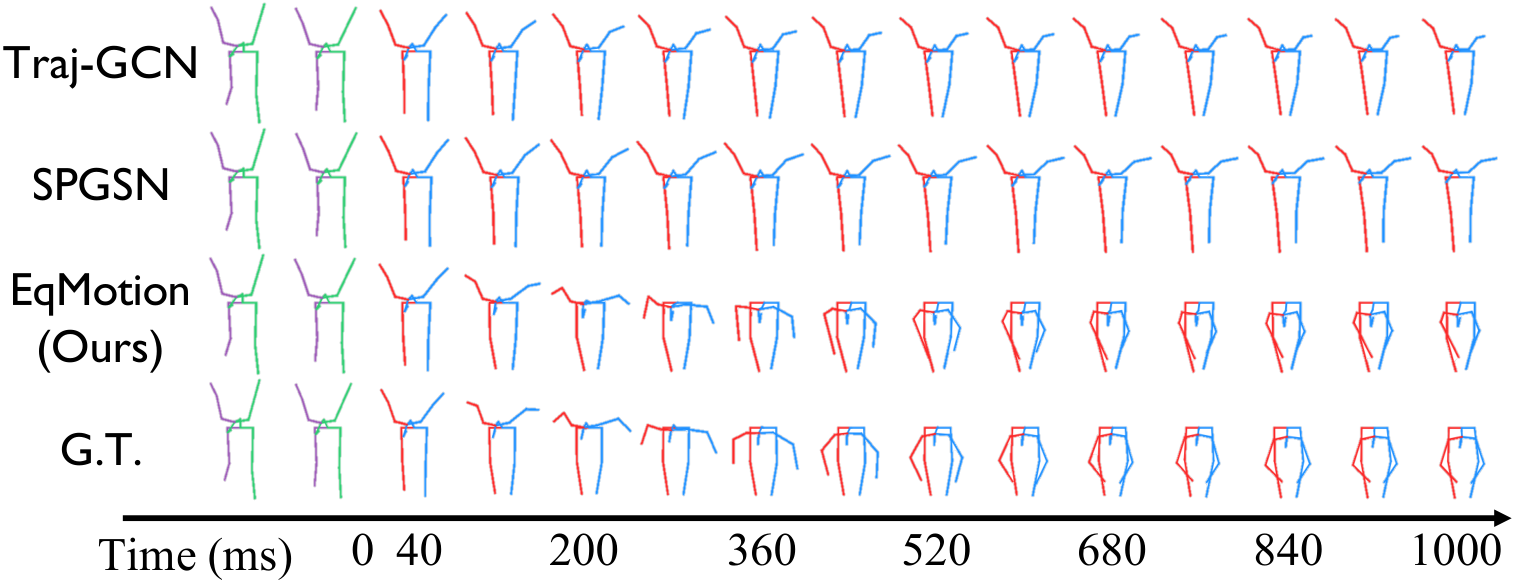
Visualization results Figure 4 visualizes and compares the predictions on H3.6M. Baselines fail to predict future movements. EqMotion completes the action more precisely.

The quantitative and visualization results reveal that EqMotion outperforms many previous methods that are task-specific, reflecting the effectiveness of EqMotion.

We conduct experiments on pedestrian trajectory prediction using the ETH-UCY dataset lerner2007crowds; pellegrini2009you, which contains 5 subsets, ETH, HOTEL, UNIV, ZARA1, and ZARA2. Following the standard setting alahi2016social; gupta2018social; yuan2021agentformer, we use 3.2 seconds (8 timestamps) to predict the 4.8 seconds (12 timestamps).

Here we apply our EqMotion to two prediction modes: deterministic and multi-prediction. Deterministic means the model only outputs a single prediction for each input motion. Multi-prediction means the model has 20 predictions for each input motion. Under multi-prediction, ADE and FDE will be calculated by the best-performed predicted motion. To adapt to multi-prediction, we slightly modify EqMotion to repeat the last feature updating layer and the output layer 20 times in parallel to have a multi-head prediction, see the details in the Appendix. Table 5 compares our method with sixteen baselines. We observe that i) EqMotion achieves state-of-the-art performance with the lowest average ADE and FDE, outperforming many baseline methods that are specifically designed for this task. EqMotion reduces the FDE by 10.4$\%$ and 7.9$\%$ under deterministic and multi-prediction settings; and ii) EqMotion achieves the best or the second best ADE/FDE result on most subsets, reflecting its effectiveness on the pedestrian trajectory prediction.

Effect of network modules We explore the effect of three proposed key modules in EqMotion on the H3.6M dataset, including the equivariant geometric feature learning (EGFL), the invariant pattern feature learning (IPFL) and the invariant reasoning module (IRM). Table 6 presents the experimental result. It is observed that i) the proposed three key modules all contribute to an accurate prediction; and ii) the equivariant geometric feature learning module is most important since learning a comprehensive equivariant geometric feature directly for prediction is the most important.

Effect of equivariant operations We explore the effect of three proposed operations in the equivariant feature learning module in EqMotion, including the inner-agent attention (Inner att), inter-agent aggregation (Inter agg) and non-linear function (Non-linear). Table 7 presents the results. We see that the proposed three key operations all contribute to promoting an accurate prediction.

Different amounts of training data Figure 5 presents the comparison of model performance under different amounts of training data on H3.6M. We see that i) our method achieves the best prediction performance under all training data ratios; and ii) our method even outperforms some full-data using baselines by only using 5$\%$ of training data since the equivariant design promotes the network generalization ability under Euclidean transformations.

Model size Figure 6 compares EqMotion to existing methods in terms of the model size and prediction results in short-term prediction on H3.6M. We can observe that EqMotion has the smallest model size (less than 30% of other models’ sizes) with the lowest MPJPE thanks to the equivariant design that compacts the model free from generalizing over rotations and translations of the data.

References

- (1) Alexandre Alahi, Kratarth Goel, Vignesh Ramanathan, Alexandre Robicquet, Li Fei-Fei, and Silvio Savarese. Social lstm: Human trajectory prediction in crowded spaces. In Proceedings of the IEEE conference on computer vision and pattern recognition, pages 961–971, 2016.
- (2) Inhwan Bae, Jin-Hwi Park, and Hae-Gon Jeon. Learning pedestrian group representations for multi-modal trajectory prediction. In European Conference on Computer Vision, pages 270–289. Springer, 2022.
- (3) Peter Battaglia, Razvan Pascanu, Matthew Lai, Danilo Jimenez Rezende, et al. Interaction networks for learning about objects, relations and physics. Advances in neural information processing systems, 29, 2016.
- (4) Yujun Cai, Lin Huang, Yiwei Wang, Tat-Jen Cham, Jianfei Cai, Junsong Yuan, Jun Liu, Xu Yang, Yiheng Zhu, Xiaohui Shen, et al. Learning progressive joint propagation for human motion prediction. In European Conference on Computer Vision, pages 226–242. Springer, 2020.
- (5) Sergio Casas, Wenjie Luo, and Raquel Urtasun. Intentnet: Learning to predict intention from raw sensor data. In Conference on Robot Learning, pages 947–956. PMLR, 2018.
- (6) Yuning Chai, Benjamin Sapp, Mayank Bansal, and Dragomir Anguelov. Multipath: Multiple probabilistic anchor trajectory hypotheses for behavior prediction. arXiv preprint arXiv:1910.05449, 2019.
- (7) Stefan Chmiela, Alexandre Tkatchenko, Huziel E Sauceda, Igor Poltavsky, Kristof T Schütt, and Klaus-Robert Müller. Machine learning of accurate energy-conserving molecular force fields. Science advances, 3(5):e1603015, 2017.
- (8) Taco Cohen and Max Welling. Group equivariant convolutional networks. In International conference on machine learning, pages 2990–2999. PMLR, 2016.
- (9) Lingwei Dang, Yongwei Nie, Chengjiang Long, Qing Zhang, and Guiqing Li. Msr-gcn: Multi-scale residual graph convolution networks for human motion prediction. In Proceedings of the IEEE/CVF International Conference on Computer Vision, pages 11467–11476, 2021.
- (10) Congyue Deng, Or Litany, Yueqi Duan, Adrien Poulenard, Andrea Tagliasacchi, and Leonidas J Guibas. Vector neurons: A general framework for so (3)-equivariant networks. In Proceedings of the IEEE/CVF International Conference on Computer Vision, pages 12200–12209, 2021.
- (11) Carlos Esteves, Christine Allen-Blanchette, Xiaowei Zhou, and Kostas Daniilidis. Polar transformer networks. arXiv preprint arXiv:1709.01889, 2017.
- (12) Marc Finzi, Samuel Stanton, Pavel Izmailov, and Andrew Gordon Wilson. Generalizing convolutional neural networks for equivariance to lie groups on arbitrary continuous data. In International Conference on Machine Learning, pages 3165–3176. PMLR, 2020.
- (13) Katerina Fragkiadaki, Sergey Levine, Panna Felsen, and Jitendra Malik. Recurrent network models for human dynamics. In Proceedings of the IEEE international conference on computer vision, pages 4346–4354, 2015.
- (14) Fabian Fuchs, Daniel Worrall, Volker Fischer, and Max Welling. Se (3)-transformers: 3d roto-translation equivariant attention networks. Advances in Neural Information Processing Systems, 33:1970–1981, 2020.
- (15) Jiyang Gao, Chen Sun, Hang Zhao, Yi Shen, Dragomir Anguelov, Congcong Li, and Cordelia Schmid. Vectornet: Encoding hd maps and agent dynamics from vectorized representation. In Proceedings of the IEEE/CVF Conference on Computer Vision and Pattern Recognition, pages 11525–11533, 2020.
- (16) Francesco Giuliari, Irtiza Hasan, Marco Cristani, and Fabio Galasso. Transformer networks for trajectory forecasting. In 2020 25th International Conference on Pattern Recognition (ICPR), pages 10335–10342. IEEE, 2021.
- (17) Colin Graber and Alexander G Schwing. Dynamic neural relational inference. In Proceedings of the IEEE/CVF Conference on Computer Vision and Pattern Recognition, pages 8513–8522, 2020.
- (18) Tianpei Gu, Guangyi Chen, Junlong Li, Chunze Lin, Yongming Rao, Jie Zhou, and Jiwen Lu. Stochastic trajectory prediction via motion indeterminacy diffusion. In Proceedings of the IEEE/CVF Conference on Computer Vision and Pattern Recognition, pages 17113–17122, 2022.
- (19) Xiao Guo and Jongmoo Choi. Human motion prediction via learning local structure representations and temporal dependencies. In Proceedings of the AAAI Conference on Artificial Intelligence, volume 33, pages 2580–2587, 2019.
- (20) Agrim Gupta, Justin Johnson, Li Fei-Fei, Silvio Savarese, and Alexandre Alahi. Social gan: Socially acceptable trajectories with generative adversarial networks. In Proceedings of the IEEE Conference on Computer Vision and Pattern Recognition, pages 2255–2264, 2018.
- (21) Dirk Helbing and Peter Molnar. Social force model for pedestrian dynamics. Physical review E, 51(5):4282, 1995.
- (22) Yue Hu, Siheng Chen, Ya Zhang, and Xiao Gu. Collaborative motion prediction via neural motion message passing. In Proceedings of the IEEE/CVF Conference on Computer Vision and Pattern Recognition, pages 6319–6328, 2020.
- (23) Wenbing Huang, Jiaqi Han, Yu Rong, Tingyang Xu, Fuchun Sun, and Junzhou Huang. Equivariant graph mechanics networks with constraints. arXiv preprint arXiv:2203.06442, 2022.
- (24) Michael J Hutchinson, Charline Le Lan, Sheheryar Zaidi, Emilien Dupont, Yee Whye Teh, and Hyunjik Kim. Lietransformer: Equivariant self-attention for lie groups. In International Conference on Machine Learning, pages 4533–4543. PMLR, 2021.
- (25) Catalin Ionescu, Dragos Papava, Vlad Olaru, and Cristian Sminchisescu. Human3. 6m: Large scale datasets and predictive methods for 3d human sensing in natural environments. IEEE transactions on pattern analysis and machine intelligence, 36(7):1325–1339, 2013.
- (26) Ashesh Jain, Amir R Zamir, Silvio Savarese, and Ashutosh Saxena. Structural-rnn: Deep learning on spatio-temporal graphs. In Proceedings of the ieee conference on computer vision and pattern recognition, pages 5308–5317, 2016.
- (27) Bowen Jing, Stephan Eismann, Patricia Suriana, Raphael JL Townshend, and Ron Dror. Learning from protein structure with geometric vector perceptrons. arXiv preprint arXiv:2009.01411, 2020.
- (28) Thomas Kipf, Ethan Fetaya, Kuan-Chieh Wang, Max Welling, and Richard Zemel. Neural relational inference for interacting systems. In International Conference on Machine Learning, pages 2688–2697. PMLR, 2018.
- (29) Kris M Kitani, Brian D Ziebart, James Andrew Bagnell, and Martial Hebert. Activity forecasting. In European conference on computer vision, pages 201–214. Springer, 2012.
- (30) Miltiadis Kofinas, Naveen Nagaraja, and Efstratios Gavves. Roto-translated local coordinate frames for interacting dynamical systems. Advances in Neural Information Processing Systems, 34:6417–6429, 2021.
- (31) Jonas Köhler, Leon Klein, and Frank Noé. Equivariant flows: sampling configurations for multi-body systems with symmetric energies. arXiv preprint arXiv:1910.00753, 2019.
- (32) Namhoon Lee, Wongun Choi, Paul Vernaza, Christopher B Choy, Philip HS Torr, and Manmohan Chandraker. Desire: Distant future prediction in dynamic scenes with interacting agents. In Proceedings of the IEEE Conference on Computer Vision and Pattern Recognition, pages 336–345, 2017.
- (33) Andreas M Lehrmann, Peter V Gehler, and Sebastian Nowozin. Efficient nonlinear markov models for human motion. In Proceedings of the IEEE Conference on Computer Vision and Pattern Recognition, pages 1314–1321, 2014.
- (34) Alon Lerner, Yiorgos Chrysanthou, and Dani Lischinski. Crowds by example. In Computer graphics forum, volume 26, pages 655–664. Wiley Online Library, 2007.
- (35) Jesse Levinson, Jake Askeland, Jan Becker, Jennifer Dolson, David Held, Soeren Kammel, J Zico Kolter, Dirk Langer, Oliver Pink, Vaughan Pratt, et al. Towards fully autonomous driving: Systems and algorithms. In 2011 IEEE intelligent vehicles symposium (IV), pages 163–168. IEEE, 2011.
- (36) Chen Li, Zhen Zhang, Wee Sun Lee, and Gim Hee Lee. Convolutional sequence to sequence model for human dynamics. In Proceedings of the IEEE Conference on Computer Vision and Pattern Recognition, pages 5226–5234, 2018.
- (37) Jiachen Li, Fan Yang, Masayoshi Tomizuka, and Chiho Choi. Evolvegraph: Multi-agent trajectory prediction with dynamic relational reasoning. Proceedings of the Neural Information Processing Systems (NeurIPS), 2020.
- (38) Maosen Li, Siheng Chen, Xu Chen, Ya Zhang, Yanfeng Wang, and Qi Tian. Actional-structural graph convolutional networks for skeleton-based action recognition. In Proceedings of the IEEE/CVF conference on computer vision and pattern recognition, pages 3595–3603, 2019.
- (39) Maosen Li, Siheng Chen, Xu Chen, Ya Zhang, Yanfeng Wang, and Qi Tian. Symbiotic graph neural networks for 3d skeleton-based human action recognition and motion prediction. IEEE Transactions on Pattern Analysis and Machine Intelligence, 44(6):3316–3333, 2021.
- (40) Maosen Li, Siheng Chen, Zijing Zhang, Lingxi Xie, Qi Tian, and Ya Zhang. Skeleton-parted graph scattering networks for 3d human motion prediction. In European Conference on Computer Vision, 2022.
- (41) Maosen Li, Siheng Chen, Yangheng Zhao, Ya Zhang, Yanfeng Wang, and Qi Tian. Dynamic multiscale graph neural networks for 3d skeleton based human motion prediction. In Proceedings of the IEEE/CVF Conference on Computer Vision and Pattern Recognition, pages 214–223, 2020.
- (42) Junwei Liang, Lu Jiang, Kevin Murphy, Ting Yu, and Alexander Hauptmann. The garden of forking paths: Towards multi-future trajectory prediction. In Proceedings of the IEEE/CVF Conference on Computer Vision and Pattern Recognition, pages 10508–10518, 2020.
- (43) Ming Liang, Bin Yang, Rui Hu, Yun Chen, Renjie Liao, Song Feng, and Raquel Urtasun. Learning lane graph representations for motion forecasting. In European Conference on Computer Vision, pages 541–556. Springer, 2020.
- (44) Tiezheng Ma, Yongwei Nie, Chengjiang Long, Qing Zhang, and Guiqing Li. Progressively generating better initial guesses towards next stages for high-quality human motion prediction. In Proceedings of the IEEE/CVF Conference on Computer Vision and Pattern Recognition, pages 6437–6446, 2022.
- (45) Karttikeya Mangalam, Harshayu Girase, Shreyas Agarwal, Kuan-Hui Lee, Ehsan Adeli, Jitendra Malik, and Adrien Gaidon. It is not the journey but the destination: Endpoint conditioned trajectory prediction. In European Conference on Computer Vision, pages 759–776. Springer, 2020.
- (46) Wei Mao, Miaomiao Liu, and Mathieu Salzmann. History repeats itself: Human motion prediction via motion attention. In European Conference on Computer Vision, pages 474–489. Springer, 2020.
- (47) Wei Mao, Miaomiao Liu, Mathieu Salzmann, and Hongdong Li. Learning trajectory dependencies for human motion prediction. In Proceedings of the IEEE/CVF International Conference on Computer Vision, pages 9489–9497, 2019.
- (48) Francesco Marchetti, Federico Becattini, Lorenzo Seidenari, and Alberto Del Bimbo. Mantra: Memory augmented networks for multiple trajectory prediction. In Proceedings of the IEEE/CVF Conference on Computer Vision and Pattern Recognition, pages 7143–7152, 2020.
- (49) Diego Marcos, Michele Volpi, Nikos Komodakis, and Devis Tuia. Rotation equivariant vector field networks. In Proceedings of the IEEE International Conference on Computer Vision, pages 5048–5057, 2017.
- (50) Julieta Martinez, Michael J Black, and Javier Romero. On human motion prediction using recurrent neural networks. In Proceedings of the IEEE conference on computer vision and pattern recognition, pages 2891–2900, 2017.
- (51) Ramin Mehran, Alexis Oyama, and Mubarak Shah. Abnormal crowd behavior detection using social force model. In 2009 IEEE Conference on Computer Vision and Pattern Recognition, pages 935–942. IEEE, 2009.
- (52) Jeremy Morton, Tim A Wheeler, and Mykel J Kochenderfer. Analysis of recurrent neural networks for probabilistic modeling of driver behavior. IEEE Transactions on Intelligent Transportation Systems, 18(5):1289–1298, 2016.
- (53) Damian Mrowca, Chengxu Zhuang, Elias Wang, Nick Haber, Li F Fei-Fei, Josh Tenenbaum, and Daniel L Yamins. Flexible neural representation for physics prediction. Advances in neural information processing systems, 31, 2018.
- (54) Stefano Pellegrini, Andreas Ess, Konrad Schindler, and Luc Van Gool. You’ll never walk alone: Modeling social behavior for multi-target tracking. In 2009 IEEE 12th International Conference on Computer Vision, pages 261–268. IEEE, 2009.
- (55) Tim Salzmann, Boris Ivanovic, Punarjay Chakravarty, and Marco Pavone. Trajectron++: Multi-agent generative trajectory forecasting with heterogeneous data for control. 2020.
- (56) Alvaro Sanchez-Gonzalez, Victor Bapst, Kyle Cranmer, and Peter Battaglia. Hamiltonian graph networks with ode integrators. arXiv preprint arXiv:1909.12790, 2019.
- (57) Alvaro Sanchez-Gonzalez, Jonathan Godwin, Tobias Pfaff, Rex Ying, Jure Leskovec, and Peter Battaglia. Learning to simulate complex physics with graph networks. In International Conference on Machine Learning, pages 8459–8468. PMLR, 2020.
- (58) Vıctor Garcia Satorras, Emiel Hoogeboom, and Max Welling. E (n) equivariant graph neural networks. In International conference on machine learning, pages 9323–9332. PMLR, 2021.
- (59) Bohan Tang, Yiqi Zhong, Ulrich Neumann, Gang Wang, Ya Zhang, and Siheng Chen. Collaborative uncertainty in multi-agent trajectory forecasting. Advances in Neural Information Processing Systems, 34, 2021.
- (60) Graham W Taylor and Geoffrey E Hinton. Factored conditional restricted boltzmann machines for modeling motion style. In Proceedings of the 26th annual international conference on machine learning, pages 1025–1032, 2009.
- (61) Nathaniel Thomas, Tess Smidt, Steven Kearnes, Lusann Yang, Li Li, Kai Kohlhoff, and Patrick Riley. Tensor field networks: Rotation-and translation-equivariant neural networks for 3d point clouds. arXiv preprint arXiv:1802.08219, 2018.
- (62) Benjamin Ummenhofer, Lukas Prantl, Nils Thuerey, and Vladlen Koltun. Lagrangian fluid simulation with continuous convolutions. In International Conference on Learning Representations, 2019.
- (63) Anirudh Vemula, Katharina Muelling, and Jean Oh. Social attention: Modeling attention in human crowds. In 2018 IEEE international Conference on Robotics and Automation (ICRA), pages 4601–4607. IEEE, 2018.
- (64) Jacob Walker, Kenneth Marino, Abhinav Gupta, and Martial Hebert. The pose knows: Video forecasting by generating pose futures. In Proceedings of the IEEE international conference on computer vision, pages 3332–3341, 2017.
- (65) Jack M Wang, David J Fleet, and Aaron Hertzmann. Gaussian process dynamical models for human motion. IEEE transactions on pattern analysis and machine intelligence, 30(2):283–298, 2007.
- (66) Maurice Weiler, Fred A Hamprecht, and Martin Storath. Learning steerable filters for rotation equivariant cnns. In Proceedings of the IEEE Conference on Computer Vision and Pattern Recognition, pages 849–858, 2018.
- (67) Daniel E Worrall, Stephan J Garbin, Daniyar Turmukhambetov, and Gabriel J Brostow. Harmonic networks: Deep translation and rotation equivariance. In Proceedings of the IEEE Conference on Computer Vision and Pattern Recognition, pages 5028–5037, 2017.
- (68) Chenxin Xu, Siheng Chen, Maosen Li, and Ya Zhang. Invariant teacher and equivariant student for unsupervised 3d human pose estimation. In Proceedings of the AAAI Conference on Artificial Intelligence, volume 35, pages 3013–3021, 2021.
- (69) Chenxin Xu, Maosen Li, Zhenyang Ni, Ya Zhang, and Siheng Chen. Groupnet: Multiscale hypergraph neural networks for trajectory prediction with relational reasoning. In Proceedings of the IEEE/CVF Conference on Computer Vision and Pattern Recognition, pages 6498–6507, 2022.
- (70) Chenxin Xu, Weibo Mao, Wenjun Zhang, and Siheng Chen. Remember intentions: Retrospective-memory-based trajectory prediction. In Proceedings of the IEEE/CVF Conference on Computer Vision and Pattern Recognition, pages 6488–6497, 2022.
- (71) Chenxin Xu, Yuxi Wei, Bohan Tang, Sheng Yin, Ya Zhang, and Siheng Chen. Dynamic-group-aware networks for multi-agent trajectory prediction with relational reasoning. arXiv preprint arXiv:2206.13114, 2022.
- (72) Xingyi Yang, Jingwen Ye, and Xinchao Wang. Factorizing knowledge in neural networks. In European Conference on Computer Vision, 2022.
- (73) Xingyi Yang, Daquan Zhou, Songhua Liu, Jingwen Ye, and Xinchao Wang. Deep model reassembly. In Conference on Neural Information Processing Systems, 2022.
- (74) Yiding Yang, Zunlei Feng, Mingli Song, and Xinchao Wang. Factorizable graph convolutional networks. In Conference on Neural Information Processing Systems, 2020.
- (75) Yiding Yang, Jiayan Qiu, Mingli Song, Dacheng Tao, and Xinchao Wang. Distilling knowledge from graph convolutional networks. In Proceedings of the IEEE/CVF Conference on Computer Vision and Pattern Recognition, 2020.
- (76) Ye Yuan, Xinshuo Weng, Yanglan Ou, and Kris M Kitani. Agentformer: Agent-aware transformers for socio-temporal multi-agent forecasting. In Proceedings of the IEEE/CVF International Conference on Computer Vision, pages 9813–9823, 2021.
- (77) Yiqi Zhong, Zhenyang Ni, Siheng Chen, and Ulrich Neumann. Aware of the history: Trajectory forecasting with the local behavior data. In Computer Vision–ECCV 2022: 17th European Conference, Tel Aviv, Israel, October 23–27, 2022, Proceedings, Part XXII, pages 393–409. Springer, 2022.
Appendix A Theoretical Proofs
In this section, we prove Theorem 1 in our paper which shows EqMotion’s equivariance property and the interaction reasoning module’s invariance property. Note that, here we treat all the vectors to be row vectors since we multiply the rotation matrix by right.
1. For the initialization layer , the initial geometric feature is equivariant and the initial pattern feature is invariant:
Proof: For the th agent, we show its initial geometric feature is equivariant to the input motion under Euclidean transformation. When transforming the past motion, we have