LNO: Laplace Neural Operator for Solving Differential Equations

To implement the proposed LNO, the input function $\mathbf{f}(t)\in\mathbb{R}_{d_{x}}$ is first transformed into a higher dimensional representation $v(t)\in\mathbb{R}_{d_{z}}$ using a lifting layer, denoted by $\mathcal{P}$. This layer is typically realized by a shallow neural network or a linear transformation. Next, a nonlinear operator is applied to this representation using the sum of the Laplace layer and a bias function in a neural network architecture as:

where $\sigma$ is a nonlinear activation function, $\mathbf{W}$ is a linear transformation, and $\kappa$ is a kernel integral transformation. Lastly, the output $\mathbf{x}(t)$ is obtained by projecting $u(t)$ through a local transformation layer, $\mathcal{Q}$. In Eq. 5, the kernel integral operator mapping is denoted as:

where $\kappa_{\phi}$ is a neural network parameterized by $\phi$. If we remove the dependence on the function $\mathbf{f}$ and impose $\kappa_{\phi}(t,\tau)=\kappa_{\phi}(t-\tau)$, Eq. 5 becomes a convolution operator:

Now in the next section, we build the relationship between the Laplace transform of the input function and the Laplace transform of the output function employing the Pole-residue formulation in the Laplace layer.

We propose to replace the kernel integral operator in Eq. 7 with an operator defined in the Laplace domain. By taking the Laplace transform of Eq. 7, we get

where $\mathscr{L}\{.\}$ and $\mathscr{L}^{-1}\{.\}$ are operators of the Laplace transform and inverse Laplace transform, respectively; $K_{\phi}(s)=\mathscr{L}\{\kappa_{\phi}(t)\}$ and $V(s)=\mathscr{L}\{v(t)\}$. We express $K_{\phi}(s)$ in the pole-residue form:

Here, we propose to choose $K_{\phi}$ to be a neural network directly parameterized by: $\bm{\theta}=(\mu_{1},\cdots,\mu_{N},\beta_{1},\cdots,\beta_{N})$ in the Laplace domain, where $\mu_{n}$ and $\beta_{n}$ are the trainable system poles and residues, respectively. An irregular excitation signal $v(t)$ with period $T$ can be decomposed into its Fourier series:

where $\omega_{\ell}=\ell\omega_{1}$, $\omega_{1}$ is the fundamental frequency in rad$/$s, and $\alpha_{\ell}$ is the complex Fourier coefficient. Taking the Laplace transform of Eq. (10) yields:

From $U(s)=K_{\phi}(s)V(s)$, using Eqs. 9 and 11, one writes

Expressing Eq. 12 in a pole-residue form yields cao2023laplace, hu2016pole

From Eqs. 12 and 13, the response residues corresponding to the first $N$ response poles (i.e., at the system poles, $\mu_{n}$) can be obtained by the residue theorem kreyszig2010advanced:

where

Similarly, the response residues corresponding to the last response poles (i.e., at the excitation poles, $i\omega_{\ell}$) are

where

Once $\gamma_{n}$ and $\lambda_{\ell}$ are obtained, by taking the inverse Laplace transform of Eq. 13, we obtain:

In Eq. 18, the first summation term of the right-hand side is the transient response related to the system poles. The second summation term of the right-hand side is the familiar steady-state response operated in the frequency domain.

The Duffing equation is a non-linear second-order differential equation used to model certain damped and driven oscillators. The Duffing oscillator is an example of a forced oscillator with nonlinear elasticity, and can be written as:

where $f(t)$ is the externally applied force, $m$, $c$ are the mass, damping coefficients, $k_{1}$ and $k_{3}$ stiffness of the system, and $x(t)$, $\dot{x}(t)$ and $\ddot{x}(t)$ are the displacement, velocity, and acceleration of the dynamic response, respectively. Eq. 19 is subjected to zero initial conditions $x(0)=0$ and $\dot{x}(0)=0$, and the damping coefficient, $c\geq 0$. The Duffing oscillator is one of the prototype systems of nonlinear dynamics, which has been successfully utilized to model many processes, such as beam buckling, stiffening springs, and ionization waves in plasmas.

In this example, for simplicity we have considered $m=1$, $k_{1}=1$, and $k_{3}=1$, and have studied two scenarios:

• 1.

  Scenario $1$: A Duffing oscillator that does not include damping, i.e., $c=0$.

• 2.

  Scenario $2$: A Duffing oscillator that includes a damping term with the coefficient $c=0.5$.

Here, our goal is to learn the non-linear operator of the system in Eq. 19, which maps the forcing function, $f(t)$ (considered as input) to the system response denoted by $x(t)$; that is, $\mathcal{G}_{\bm{\theta}}:f(t)\rightarrow x(t)$. To generate $N_{train}$ samples to train LNO, we consider a sinusoidal forcing function, $f_{train}(t)=Asin(5t)$, where the amplitude $A\in[0.05,10]$ with an interval $\delta A=0.05$, therefore $N_{train}=200$. Each sample is discretized into $2048$ temporal points and the time interval is $\Delta t=0.01$ seconds. The response is calculated by a versatile ODE solver—$\mathbf{ode45}$ on MATLAB. For validating and testing the neural operator, we generated datasets considering a decaying sinusoidal forcing function, $f_{test}(t)=Ae^{-0.05t}sin(5t)$, where the amplitude $A\in[0.14,9.09]$ and $N_{vali}=50$ and $N_{test}=130$.

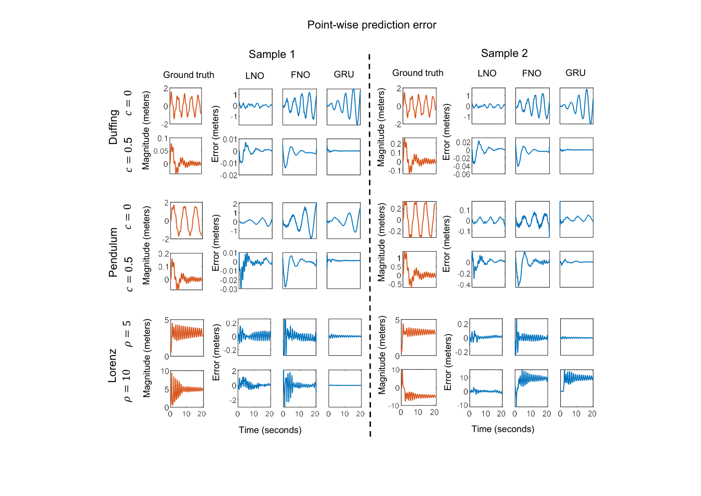
The results presented in Fig. 3 demonstrate that LNO approximates the test cases of scenarios $1$ and $2$ with overall high accuracy. The improvement of the prediction of LNO over FNO is more pronounced for oscillators without damping (Scenario $1$: the first column of Fig. 3). If the damping of a system is zero, there will always exist a transient response. The approximation accuracy of LNO is better than FNO because it can capture both steady-state and transient responses, although it has a higher standard deviation. LNO is more accurate than GRU when there is no damping, but GRU is more accurate than LNO when the damping term is introduced, $c=0.5$. The batch size used for LNO affects its results, so choosing an appropriate value is essential. Fig. 4 (first and second rows) presents the error plots of two representative test samples for each of the neural models. Additionally, a visual representation of the prediction of the solution obtained from the two neural operators for both scenarios is shown in Fig. 5. Figs. 5 (a) and (c) illustrate that the generalization gap of FNO (the difference between a model’s performance on training data and its performance on unseen data) is significantly higher than that of LNO.

In the next example, we consider a gravity pendulum subjected to an external force, $f(t)$. The equation which describes the motion of the pendulum is written as:

where $g$ is the magnitude of the gravitational field, $l$ is the length of the rod; $c$ is the damping due to friction; $x$ is the angle from the vertical to the pendulum; and $f(t)$ is the external force. For simplicity, we have chosen $g/l=1$ in this example, and the following two scenarios are also considered:

• 1.

  Scenario $1$: the pendulum does not include damping, i.e., $c=0$.

• 2.

  Scenario $2$: the pendulum includes a damping term with the coefficient $c=0.5$.

For the driven gravity pendulum model, we consider the same forcing functions for training, $f_{train}$, and testing, $f_{test}$ as used in Section 3.1. Thus, $N_{train}=200$, $N_{vali}=50$, and $N_{test}=130$. The corresponding responses, $x(t)$ are also computed by $\mathbf{ode45}$. We aim to learn the mapping from the external force to the motion of the pendulum, that is, $G_{\bm{\theta}}:f(t)\rightarrow x(t)$. The third and the fourth columns of Fig. 3 show the relative $\mathcal{L}_{2}$ errors of the predictions computed by the LNO, FNO, and GRU for both scenarios. As observed in the previous example, LNO can predict the results more accurately than FNO and GRU for the systems without damping. Fig. 4 (third and fourth rows) presents the error plots of two representative test samples for each of the neural models. Additionally, a visual representation of the prediction of the solution obtained from the two neural operators for both scenarios is shown in Fig. 6.

This example is the last ODE considered in this work. The Lorentz system is a mathematical model that simplifies many practical problems, including electric circuits, atmospheric convection, and forward osmosis. In this case, we are studying a forced Lorenz system, which has a forcing term and may be more practical. For instance, climate studies can use this system to model the temperature of the atmosphere and oceans as forcing terms shi2021analysis. The forced Lorenz system includes three ODEs defined as:

where $x$ is proportional to the rate of convection, $y$ is proportional to the horizontal temperature variation; $z$ is proportional to the vertical temperature variation. The terms $\sigma$, $\rho$, and $\beta$ are three constant parameters related to the Prandtl number, Rayleigh number, and specific physical dimensions of the layer, respectively. Even though the equations are simple, the Lorenz system has chaotic and unpredictable behavior, so it is highly sensitive to initial conditions. The initial conditions in this example are chosen slightly away from the state of no convection, that is $x(0)=1$, $y(0)=0$, $z(0)=0$. The $\sigma=10$ and $\beta=8/3$ are chosen in this example. We consider the following two scenarios:

• 1.

  Scenario $1$: Rayleigh number $\rho=5$.

• 2.

  Scenario $2$: Rayleigh number $\rho=10$.

The number of samples for training, testing, and validation is kept the same as in the previous two examples. We aim to learn the mapping from the source term, $f(t)$ to the system response, $x(t)$. The results presented in Fig. 3 (last two columns) demonstrate that LNO approximates the test cases of scenarios $1$ and $2$ with overall high accuracy. The improvement of the accuracy is more pronounced in the case of $\rho=10$, as we observe that the response has two patterns, which are shown in the ground truth of the last row of Fig. 4. Figs. 7 (a) and (c) illustrate that the generalization gap of FNO is significantly higher than that of LNO. Fig. 4 (last two rows) presents the error plots of two representative test samples for each of the neural models. Additionally, a visual representation of the prediction of the solution obtained from the two neural operators for both scenarios is shown in Fig. 7.

For a dynamic $1D$ Euler-Bernoulli beam, the Euler-Lagrange equation is written as:

where $y(x,t)$ is the deflection of the beam at the location $x$ and time $t$; $f(x,t)$ is the source term; $E$ and $I$ are the elastic modulus and the second moment of area of the cross-section of the beam, respectively; $\rho$ and $A$ are the material density and the area of the cross-section of the beam, respectively.

Here, our goal is to learn the operator of the system in Eq. 23, which maps the source, $f(x,t)$, to the steady-state response $y(x,t)$; that is, $\mathcal{G}_{\bm{\theta}}:f(x,t)\rightarrow y(x,t)$. To generate $N_{train}$ samples to train LNO, we consider a function, $f_{train}(x,t)=Ae^{-0.05x}(1-10^{2})sin(10t)$, where the amplitude $A\in[0.05,10]$ with an interval $\delta A=0.05$, therefore $N_{train}=200$. Each sample is discretized into $51\times 17$ temporal-spatial grid points such that the time interval, $\Delta t=0.02$ seconds, and the spatial interval, $\Delta x=0.1$ meters. For validating and testing the neural operator, a function, $f_{test}(x,t)=Ae^{-x}(1-10^{2})sin(10t)$, is considered, where the amplitude $A\in[1.24,10.19]$ and $N_{vali}=50$ and $N_{test}=130$. While the analytical particular solution of Eq. 23 to $f_{train}$ is $y_{train}(x,t)=Ae^{-0.05x}sin(10t)$, the analytical particular solution to $f_{test}$ is $y_{test}(x,t)=Ae^{-x}sin(10t)$.

The third column from the end in Fig. 3 illustrates that the results predicted by LNO have an overall high accuracy than FNO. Fig. 8 (first and second rows) presents the error plots of two representative test samples for each of the neural models. The errors of LNO are more than an order of magnitude smaller than those of FNO.

The diffusion equation is a PDE that is applied in many fields, such as information theory, material science, and biophysics. It is a special case of the convection-diffusion equation, which describes the macroscopic behavior of lots of micro-particles in Brownian motion. The equation is usually written as:

where $y(x,t)$ describes the density of the diffusing material at location $x$ and time $t$; $f(x,t)$ is the source term; $D$ is the collective diffusion coefficient for density $y$ at location $x$. In this case, $D=1$ is chosen. Thus, Eq. 24 is identical to the heat equation.

For learning the operator of the system in Eq. 24, we consider a function, $f_{train}(x,t)=Ae^{-0.05t}(1-\pi^{2})sin(\pi x)$, where the amplitude $A\in[0.05,10]$ with an interval $\delta A=0.05$, therefore $N_{train}=200$. Each sample is discretized into $25\times 80$ temporal-spatial grid points such that the time interval, $\Delta t=0.02$ seconds, and the spatial interval, $\Delta x=0.05$ meters. For validating and testing the neural operators, we generate a dataset considering the function, $f_{test}(x,t)=Ae^{-t}(1-\pi^{2})sin(\pi x)$, where the amplitude $A\in[1.24,10.19]$ and $N_{vali}=50$ and $N_{test}=130$. The analytical particular solutions of Eq. 24 to $f_{train}$ and $f_{test}$ are $y_{train}(x,t)=Ae^{-0.05t}sin(\pi x)$ and $y_{test}(x,t)=Ae^{-t}sin(\pi x)$, respectively.

The penultimate column in Fig. 3 indicates that the predictions made by LNO exhibit a higher level of accuracy than FNO overall. Fig. 8 (rows three and four) displays error plots for two representative test samples for each neural model. The errors of LNO are two orders of magnitude smaller than those of FNO. It is worth noting that both the Euler-Bernoulli beam and the diffusion equation are essentially learning linear operators. By utilizing the linear system to accurately represent the pole-residue formulation, the results obtained with LNO in these two cases are considerably superior to those achieved with FNO.

Reaction-diffusion systems describe the change in the concentration of chemical substances or particles in time and space, which can be found in chemistry, biology, geology, and physics. The diffusion-reaction equation can be represented as:

where $y(x,t)$ represents the concentration of chemical substances or particles at location $x$ and time $t$, $f(x,t)$ is the source term and $A$ is the amplitude of the source term. In this problem, the diffusion coefficient, $D=0.01$, and the reaction rate, $k=0.01$.

We utilize the neural operators LNO and FNO to learn the mapping from the source term, $f(x,t)$ to the steady-state response $y(x,t)$, denoted as $\mathcal{G}_{\bm{\theta}}:f(x,t)\rightarrow y(x,t)$. To generate $N_{train}$ samples for training LNO, we consider a function $f_{train}(x,t)=Ae^{-0.05t}(1-\pi^{2})sin(\pi x)+A^{2}e^{-0.1t}sin(\pi x)^{2}$, where $A\in[0.05,10]$ with an interval of $\delta A=0.05$, resulting in $N_{train}=200$ samples. Each sample is discretized into $20\times 40$ temporal-spatial grid points with a time interval of $\Delta t=0.0526$ seconds and a spatial interval of $\Delta x=0.0513$. For validation and testing of the neural operator, we use a function $f_{test}(x,t)=Ae^{-t}(1-\pi^{2})sin(\pi x)+A^{2}e^{-2t}sin(\pi x)^{2}$, where $A\in[0.14,9.09]$ with $N_{vali}=50$ validation samples and $N_{test}=130$ testing samples. The analytical particular solution of $f_{train}$ for Eq. 25 is $y_{train}(x,t)=Ae^{-0.05t}sin(\pi x)$, while the analytical particular solution for $f_{test}$ is $y_{test}(x,t)=Ae^{-t}sin(\pi x)$.

The final column of Fig. 3 shows that LNO produces more accurate results overall than FNO. Fig. 8 (last two rows) displays error plots of two typical test samples for each of the neural models. LNO has smaller errors than FNO, indicating that using the poles and residues of the system as network parameters aids in operator learning, even when dealing with the steady-state response of nonlinear systems.

This work was supported by the U.S. Department of Energy, Advanced Scientific Computing Research program, under the Scalable, Efficient and Accelerated Causal Reasoning Operators, Graphs and Spikes for Earth and Embedded Systems (SEA-CROGS) project, DE- SC0023191. The authors would like to acknowledge the computing support provided by the computational resources and services at the Center for Computation and Visualization (CCV), Brown University where all experiments were carried out.

References

- [1] L. Lu, P. Jin, G. Pang, Z. Zhang, G. Karniadakis, Learning nonlinear operators via DeepONet based on the universal approximation theorem of operators, Nature Machine Intelligence 3 (3) (2021) 218–229.
- [2] Z. Li, N. Kovachki, K. Azizzadenesheli, B. Liu, K. Bhattacharya, A. Stuart, A. Anandkumar, Fourier Neural Operator for Parametric Partial Differential Equations, arXiv preprint arXiv:2010.08895 (2020).
- [3] E. Kreyszig, Advanced engineering mathematics, John Wiley & Sons, 2010.
- [4] P. R. Vlachas, J. Pathak, B. R. Hunt, T. P. Sapsis, M. Girvan, E. Ott, P. Koumoutsakos, Forecasting of spatio-temporal chaotic dynamics with recurrent neural networks: A comparative study of reservoir computing and backpropagation algorithms, arXiv preprint arXiv:1910.05266 (2019) 42.
- [5] T. Chen, H. Chen, Universal approximation to nonlinear operators by neural networks with arbitrary activation functions and its application to dynamical systems, IEEE Transactions on Neural Networks 6 (4) (1995) 911–917.
- [6] Q. Cao, S.-L. James Hu, H. Li, Laplace-and frequency-domain methods on computing transient responses of oscillators with hysteretic dampings to deterministic loading, Journal of Engineering Mechanics 149 (3) (2023) 04023005.
- [7] S.-L. J. Hu, F. Liu, B. Gao, H. Li, Pole-residue method for numerical dynamic analysis, Journal of Engineering Mechanics 142 (8) (2016) 04016045.
- [8] A. Paszke, S. Gross, F. Massa, A. Lerer, J. Bradbury, G. Chanan, T. Killeen, Z. Lin, N. Gimelshein, L. Antiga, et al., PyTorch: An Imperative Style, High-Performance Deep Learning Library, Advances in neural information processing systems 32 (2019).
- [9] A. Agarwal, P. Barham, E. Brevdo, Z. Chen, C. Citro, Tensorflow: A system for large-scale machine learning, in: Proceedings of the 12th USENIX Conference on Operating Systems Design and Implementation, USENIX Association, 2016.
- [10] Y. Shi, Analysis on averaging Lorenz system and its application to climate, Ph.D. thesis, University of Minnesota (2021).