Robust two-degrees-of-freedom control of hydraulic drive with remote wireless operation
Abstract
In this paper, a controller design targeting the remotely operated hydraulic drive system is presented. A two-degrees-of-freedom PID position controller is used, which is designed so that to maximize the integral action under robust constraint. A linearized model of the system plant, affected by the parameters uncertainties such as variable communication time-delay and overall system gain, is formulated and serves for the control design and analysis. The performed control synthesis and evaluation are targeting the remote operation where the wireless communication channel cannot secure a deterministic real-time of the control loop. The provided analysis of uncertainties makes it possible to ensure system stability under proper conditions. The theoretically expected results are confirmed through laboratory experiments on the standard industrial hydraulic components.
Index Terms:
PID controller, robust control design, hydraulic system, communication delay, remote control, robust stabilityI Introduction
Remote wireless operation, with networked control systems, become more crucial in various industries, especially due to more and more spatially distributed sensors, actuators, and different-level controllers, see e.g. a survey provided in [1]. The associated communication constraints, often expressed in varying transmission delays, see e.g. [2], will remain one of the inevitable stumbling block on the way of guaranteeing the stability and desirable level of performance of the feedback control. The latter has to be robust to specific variations in the delays and transmission intervals. Already in early two-thousands, the practical investigations were made in remote control of the mechatronic systems over communication networks, see e.g. [3]. At the same time, one can notice the recent works e.g. [4] which prioritize a robust PID design over more sensitive (to uncertainties) compensators of the time-delays, like for example the Smith predictor. The hydraulic drives, often as integrated or even embedded mechatronic systems, are becoming frequently operated in the remote and distributed plants, also via teleoperation and networked control, see e.g. [5]. Having mostly a relatively high level of the process and measurement noise and, at the same time, being safety-critical for several (often outdoor and harsh-environment) applications, also with large forces and corresponding payloads, the hydraulic drives are particularly demanding for a stable operation under the control delays and uncertainties.
In this paper, one aims to investigate a robust two-degrees-of-freedom (2DOF) PID position controller, following the methodology provided in [6] and adapting it to a complex hydraulic drive system with substantial time-delays in the control loop. Here it is worth emphasizing that our goal is not to obtain the best implementation of the remote control, so that to reduce much as possible the RTT (round trip time) in the feedback loop. Instead, one is interested rather in setting up a remotely controlled system with relatively large and variable RTT that makes the system stability more challenging. Moreover, the hydraulic systems are subject to considerable nonlinearities, as it is well known from the subject literature, see e.g. in [7, 8]. This fact makes a robust linear control design particulary challenging and relevant for the practical applications. Here, one purposefully uses the simple 2DOF PID control structure, see e.g. [9], due to its wide spread and acceptance in industries. The recent work provides experimental tests in a laboratory setting, while real industrial hydraulic components like servo-valve and linear cylinder are in use. For more details on the experimental laboratory testbed, the reader is referred to [10, 11], while the preliminary and detailed results, which are building fundament for the present work, can be found in [12].
The rest of the paper is organized as follows. Section II provides the control-oriented system modeling while emphasizing: (i) the main steps of a system linearization, (ii) its most crucial uncertainties (including time-delays), and (iii) the resulted perturbed model serving the robust control design approach. Section III is dedicated to the 2DOF PID control design. The experimental results are reported in section IV, while the brief conclusions are drawn in section V.
II Control oriented system modeling
II-A Linearized model
First, one analyzes the hydraulic system at hand. Starting from the more physical constitutive equations, a control-oriented linear system model is obtained. The hydraulic system is composed of a directional control valve (DCV), i.e. servo-valve, and a cylinder. The DCV has a nonlinear behavior due to the dead-zone and saturation of the spool stroke. Also nonlinear friction force appears when moving the piston inside the cylinder chambers. The reduced-order nonlinear model, which results from the full-order nonlinear model (see [13] for details), constitutes the basis for system linearization.
From the reduced-order model of [13] one has the equivalent orifice equation
| (1) |
where is the volumetric flow rate of hydraulic medium, is the flow coefficient (i.e. which is a valve’s constant), is the supply pressure, is the system load pressure, and is an internal variable related to the controlled state of the DCV. Recall that is subject to the dead-zone and saturation nonlinearities. One linearizes (1) for the fixed using the chain rule. Following to that, one obtains
| (2) |
with
| (3) |
and
| (4) |
In Fig. 1, one can see the block diagram of the linearized system model, from the internal control state to the output speed of the cylinder rod.

In the block diagram of Fig. 1, the following transfer function is defined
| (5) |
where is the total moving mass, is the equivalent viscous friction coefficient, is the total oil volume flowing in the hydraulic circuit, is the bulk modulus, and is the mean area of the working piston surface of the hydraulic cylinder. Self-evident is that represents the complex Laplace variable. From the block diagram of Fig. 1, one can directly compute the transfer function from to as
| (6) |
Hence, the transfer function from to results in
| (7) |
Important to notice is that is used in (5) and (6) in order to describe the linear viscous friction behavior. An appropriate choice of appears relevant because the real frictional behavior is strongly nonlinear, as confirmed with identification data shown below. Indeed, one can recognize in the velocity-force coordinates in Fig. 2, the experimentally collected data points [10] for both motion directions. Note that the points are determined each from the steady-state measurement of relative velocity and load pressure at the unidirectional drive experiments with a nearly constant speed. Recall that at steady-state, the load pressure is proportional to the total resistive force, which is due to the total friction when no other forces are in balance. The experimental data are also fitted with the Stribeck friction model, see e.g. [14, eq. (2)], which is then used for the sake of a more accurate numerical simulation. The dashed line in Fig. 2 reflects the selected linear friction coefficient . This is chosen so that the linear model reaches the same friction force level towards the end of the considered velocity range. At the same time, for the maximal possible relative velocity , detected in the open-loop experiments, the constitutes a trade-off which minimizes an integral square error between the identified Stribeck and linear viscous friction model.

Now, the obtained linear model (7) is augmented by the overall communication time delay . Therefore, one derives the overall process transfer function, i.e. from the delayed control channel to the output position of interest , as
| (8) |
Since the overall plant model has two gaining factors related to the linearization, cf. (3), (4), and one weakly-known time delay factor, one has to deal with a nominal process transfer function, for which one fixes the nominal parameter values , , . Later, those parameters are considered as a source of uncertainties in the robust control design. The nominal process transfer function is given explicitly by
| (9) |
II-B Uncertainties analysis
As shown above, the linearized gaining factors and depend on the input and state operating points and , respectively. On the other hand, the communication delay can be of a purely stochastic nature, and the only upper bound can be assumed. In order to assign the nominal values of the uncertain parameters, consider the following.
- •
In Fig. 3, the surface is shown for the sake of visualization. Since the -surface is not uniformly distributed but symmetrical with respect to the -origin, one proper choice of the nominal value is the integral mean value over the whole operative ranges, i.e. and . As it is visible from eq. (4), , so that one can stop integration at e.g. 95 % of , which is an appropriate range for the load pressure . In a similar way as , one can then assert the value for .

Fig. 3: Variations of the gaining factor . - •
In order to analyze the (RTT) delay , more than 10 different communication experiments on the hardware of experimental testbed were performed. The spatial distance between the routers of a wireless network and the intensity of the exchanged data were varied. In Fig. 4, a typical distribution determined from the measurements of is shown. Note that the 0.01 [s] column-width of the histogram corresponds the 0.01 [s] quantization of , the latter due to the communication time period captured on side of the remote controller. As can be found in the literature, see e.g. [15], [3], an RTT model for TCP/IP communication often suggests the -distribution. From Fig. 4, one can recognize that the fitted -distribution is well in accord with the measurement. Based on the determined -distribution, the nominal value is calculated as average by evaluating the integral mean value.

Fig. 4: -distribution fit of the measured distribution.
II-C Perturbed system model
The perturbed system model is defined as following
| (10) |
where is a fixed stable transfer function for weighing the uncertainties, and is a variable stable transfer function satisfying . The complex number and angular frequency are denoted by and , correspondingly. The used structure model is very well known as multiplicative perturbation. Indeed, the transfer characteristics could additionally vary from the nominal one in a range defined by in the magnitude, and by in the phase. One chooses the multiplicative perturbation structure to represent the uncertain system because of the following reasoning. From eq. (9), one can recognize that the nominal transfer function has a pair of conjugate-complex poles and a free integrator. The transfer function parameters, related to the pole pair, are the gaining factor, natural frequency, and damping coefficient
| (11) |
| (12) |
| (13) |
respectively. Following to that, one can compute the maximum relative deviation for these three parameters, which are varying subject to linearization. This is done by iterative calculation of (11), (12), (13) over the range of possible values, followed by a comparison with the parameter values obtained for the nominal . This results in
| (14) |
One can recognize that the maximal possible deviation on is significantly larger comparing to the maximal deviations of and . Such dominance in the gain variation justifies the multiplicative perturbation assumption made for the present system.
A sufficient robust stability condition for the model with the multiplicative perturbation, following to e.g. [16], is
| (15) |
where is the closed-loop transfer function. One can easily see that the robust stability (15) depends on the weighting function . Since it has to satisfy the condition (10), one can write
| (16) |
Since the multiplicative perturbation differs the and transfer functions by exactly the gaining factor and time-delay element, the inequality (16) can be transformed into, cf. [16],
| (17) |
In order to satisfy (17) for all possible , , and in the range of variations, consider the available upper bounds and . Then, one needs to find a stable transfer function which can guarantee the inequality (17) holds for the pair, so that it remains valid also for all and . Assuming the second-order lead transfer function
| (18) |
as the weighting function for robust stability (15), the parameter values , , and are fitted by minimizing the square error between and the left-hand-side of (17) for a certain range of angular frequencies around both corner frequencies of the lead element (18).
III Control design
The control design follows the methodology provided in [9], [6]. The control objectives to be achieved are:
- 1.
fast load disturbance response;
- 2.
robustness against the model uncertainties;
- 3.
robustness against the measurement noise;
- 4.
set point response accuracy.
The control solution includes the following measures:
- 1.
maximize the integral action of the PID controller;
- 2.
define a robust constraint;
- 3.
apply the second-order filter to feedback;
- 4.
tune the set point parameter and filter .
III-A Robust feedback design
The applied design algorithm [9] maximizes the integral action of the standard PID feedback controller
| (19) |
satisfying the constraint
| (20) |
The inequality (20) guarantees that the open-loop transfer function lays outside the circle of the radius , which is centered in of the complex plane. Then, it is the Nyquist theorem which guarantees the stability of the closed-loop system under this condition. Therefore, the system remains stable until surrounds . The parameter describes the robustness of the system and (20) is called a robust constraint.
If looking at the definition of the infinite norm of the sensitivity function , cf. [17], which is the maximum absolute value of over all frequencies , i.e.
| (21) |
one can write . Then, one can choose a value of according to the robustness required from the feedback control system. One assumes , cf. [9], in accord with a relatively high level of perturbations in the system.
For the identified nominal process
| (22) |
one obtains the following control gains
| (23) |
by applying the maximization algorithm proposed in [9]. In Fig. 5, one can verify the Nyquist plot of the open-loop transfer function with respect to the above robust constraint. In particular, one can see that the algorithm maximizes the PID parameters until reaching the robust constraint, i.e. by touching the -circle at three points , , , i.e. at three different angular frequencies. The resulted robust feedback control, designed for the nominal process, can be further assessed on the robust stability (15). Here, the closed-loop transfer function is multiplied with , which is satisfying (17) for . Worth noting is that while , its upper bound , cf. Fig. 4, is still satisfying the robust stability (15).

III-B 2DOF control structure
In Fig. 6, the overall 2DOF control structure is shown with
| (24) |
| (25) |
which are the feed-forward and feed-back filters, respectively. Here is the set-point parameter to be tuned, and is the parameter of the noise cutoff frequency to be adjusted for having a suitable feedback response. is set as an appropriate value, cf. [6]. is the inverse map of the orifice dead-zone, cf. [10], which has to compensate the static non-linearity which was not considered in the nominal process .

Further, compute the pre-filter, cf. [6],
| (26) |
so as to guarantee that , where , and
| (27) |
This way, the overall closed-loop transfer function, from the reference position to the output rod position, will have , hence, ensuring no overshoot in the step response.
IV Experimental results
The robust 2DOF controller, developed according to sections II and III, is experimentally evaluated on the laboratory testbed [10].

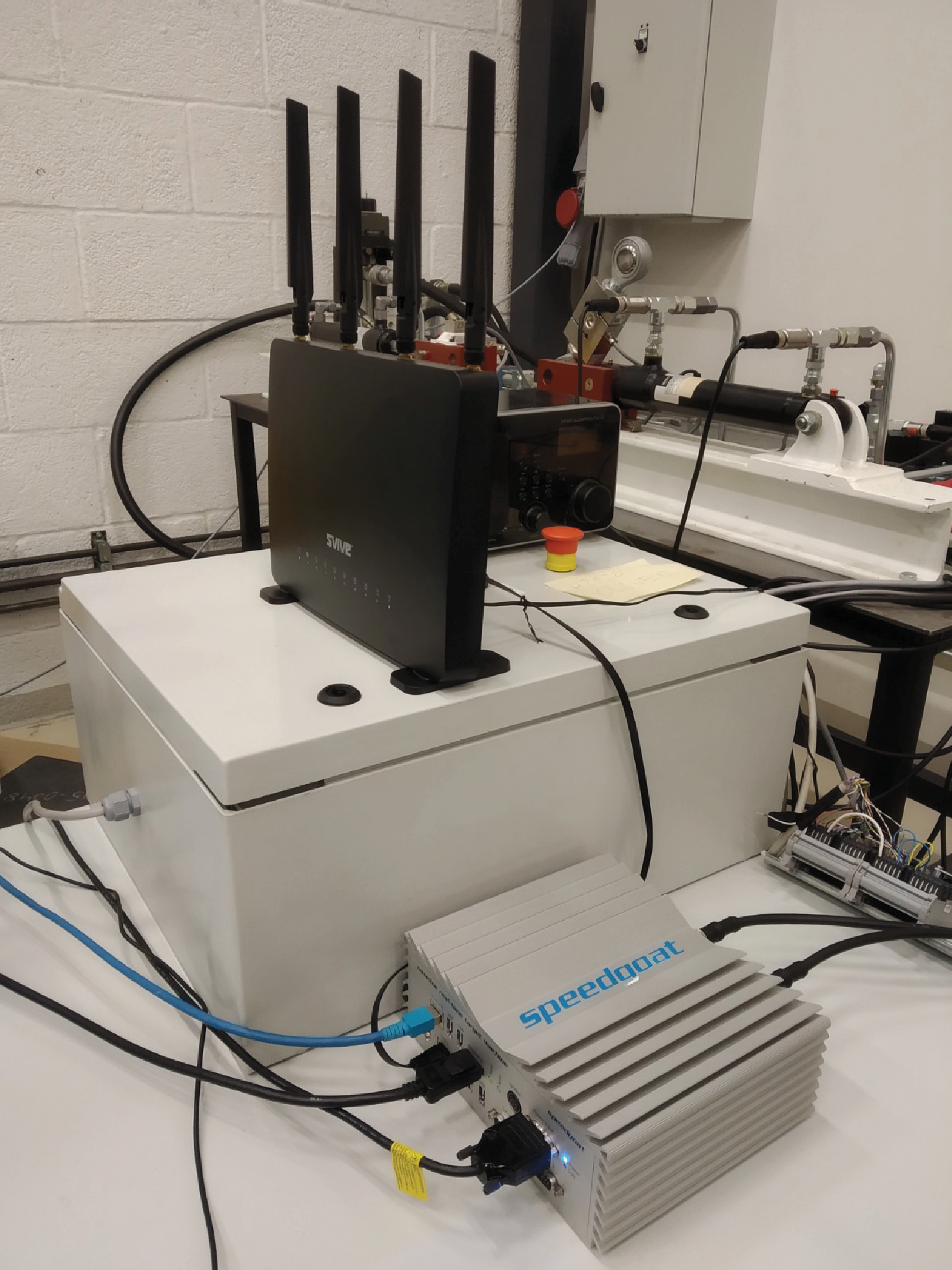
The used experimental setup is shown in Fig. 7. The real-time SpeedGoat board is controlling the power and sensor interfaces, with deterministic sampling time set to 0.0005 sec. The SpeedGoat board is connected to a standard WiFi router as a point-to-point TCP/IP communication, this way sending the measured output values, received from the sensor, and receiving the control values from a remote PC-based controller. The remote PC-based controller is realized on a standard conventional laptop computer. Due to non-real-time processes of the TCP/IP-based socket and implemented control on the running PC, the minimal possible time delay sec appears as a communication sample time.
Two communication scenarios have been evaluated: (i) the remote control communication performs via a point-to-point Ethernet connection between the real-time SpeedGoat and PC-based controller; (ii) the remote control communication performs via a wireless connection between the real-time SpeedGoat and PC-based controller by means of WiFi. Note that for (ii), various spatial distances between the WiFi communicating nodes were tested. In both communication scenarios, the RTT delay, which corresponds to the overall , was monitored and recorded in the feedback loop.


The results shown below visualize the reference and output position of the hydraulic cylinder, together with the recorded time delay in the upper plots, and the corresponding control signal in the lower plots. A series of square-pulse-shaped (with 0.1 m amplitude) positioning experiments are shown for communication scenario (i) in Fig. 8. Note that for time-delay values higher than 0.11 sec, cf. sections II and III, an instability can occur. Further it is noted that the smoothing set-point filter (26) is not applied at that stage. The same type positioning experiments for the communication scenario (ii) are shown in Fig. 9. Note that despite is transiently exceeding the value, the robustly designed 2DOF PID control maintains a stable and performant response, with solely shortcoming of transient oscillations.

In Fig. 10, the communication scenario (ii) is shown when additionally applying the set-point filter (26), cf. Fig. 6. This way, the square-pulse-shaped reference is additionally lagged, which slows down the overall output response but, in return, avoids the transient oscillations. Worth noting is that the increased spatial distance between the WiFi nodes led to the larger -variations in this case, with more frequent values closer to , cf. Figs. 8, 9, and 10.

V Conclusions
This paper shows the application of the linear 2DOF control methodology [9] to the nonlinear uncertain hydraulic drive system with significant time delays due to the wireless remote control. The robust constraint on the varying system gain and time delay parameters were specified and used for the feedback control design that meets the robust stability criteria for multiplicative disturbances. It is demonstrated in the laboratory experiments, accomplished on the standard industrial components, that the robust 2DOF PID control is well applicable to remotely operated hydraulic drives with only output measurement of the cylinder stroke.
References
- [1] P. Park, S. C. Ergen, C. Fischione, C. Lu, and K. H. Johansson, “Wireless network design for control systems: A survey,” IEEE Communications Surveys & Tutorials, vol. 20, no. 2, pp. 978–1013, 2017.
- [2] W. M. H. Heemels, A. R. Teel, N. Van de Wouw, and D. Nešić, “Networked control systems with communication constraints: Tradeoffs between transmission intervals, delays and performance,” IEEE Transactions on Automatic control, vol. 55, no. 8, pp. 1781–1796, 2010.
- [3] O. Roesch and H. Roth, “Remote control of mechatronic systems over communication networks,” in IEEE International Conference Mechatronics and Automation, 2005, pp. 1648–1653.
- [4] C. Grimholt and S. Skogestad, “Should we forget the smith predictor?” IFAC-PapersOnLine, vol. 51, no. 4, pp. 769–774, 2018.
- [5] V. Banthia, K. Zareinia, S. Balakrishnan, and N. Sepehri, “A Lyapunov stable controller for bilateral haptic teleoperation of single-rod hydraulic actuators,” Journal of Dynamic Systems, Measurement, and Control, vol. 139, no. 11, p. 111001, 2017.
- [6] H. Panagopoulos, K. Astrom, and T. Hagglund, “Design of PID controllers based on constrained optimisation,” IEE Proceedings – Control Theory and Applications, vol. 149, pp. 32–40, 2002.
- [7] H. Chaudhry, Applied Hydraulic Transients, 3rd ed. Springer, 2014.
- [8] N. Manring and R. Fales, Hydraulic Control Systems, 2nd ed. John Wiley and Sons, 2020.
- [9] K. J. Åström and T. Hägglund, Advanced PID Control. ISA - the instrumentation, systems, and automation society, 2006.
- [10] P. Pasolli and M. Ruderman, “Linearized piecewise affine in control and states hydraulic system: Modeling and identification,” in IEEE 44th Annual Conf. of Indust. Elect. Society (IECON), 2018, pp. 4537–4544.
- [11] P. Pasolli and M. Ruderman, “Hybrid position/force control for hydraulic actuators,” in IEEE 28th Mediterranean Conference on Control and Automation (MED), 2020, pp. 73–78.
- [12] R. Checchin, “Robust design of a remote motion control system for hydraulic mechatronic drive with wireless operation,” 2022, Master thesis. [Online]. Available: https://hdl.handle.net/11250/2985189
- [13] M. Ruderman, “Full- and reduced-order model of hydraulic cylinder for motion control,” in IEEE 43rd Annual Conference of the IEEE Industrial Electronics Society (IECON), 2017, pp. 7275–7280.
- [14] M. Ruderman, L. Fridman, and P. Pasolli, “Virtual sensing of load forces in hydraulic actuators using second-and higher-order sliding modes,” Control Engineering Practice, vol. 92, p. 104151, 2019.
- [15] A. Vespignani and R. Pastor-Satorras, Evolution and Structure of the Internet. Cambridge University Press, 2004.
- [16] J. Doyle, B. Francis, and A. Tannenbaum, Feedback Control Theory. Dover Publications Inc, 1990.
- [17] S. Skogestad and I. Postlethwaite, Multivariable feedback control: analysis and design, 2nd ed. John Wiley & sons, 2005.