LSwinSR: UAV Imagery Super-Resolution based on Linear Swin TransformerJournal: ISPRS Journal of Photogrammetry and Remote Sensing

Rui Li Email: rui.li.4@warwick.ac.uk Address: Intelligent Control & Smart Energy (ICSE) Research Group, School of Engineering, University of Warwick, Coventry, CV4 7AL, UK Xiaowei Zhao Email: xiaowei.zhao@warwick.ac.uk Address: Intelligent Control & Smart Energy (ICSE) Research Group, School of Engineering, University of Warwick, Coventry, CV4 7AL, UK Corresponding author: Corresponding author

Abstract

Super-resolution, which aims to reconstruct high-resolution images from low-resolution images, has drawn considerable attention and has been intensively studied in computer vision and remote sensing communities. The super-resolution technology is especially beneficial for Unmanned Aerial Vehicles (UAV), as the amount and resolution of images captured by UAV are highly limited by physical constraints such as flight altitude and load capacity. In the wake of the successful application of deep learning methods in the super-resolution task, in recent years, a series of super-resolution algorithms have been developed. In this paper, for the super-resolution of UAV images, a novel network based on the state-of-the-art Swin Transformer is proposed with better efficiency and competitive accuracy. Meanwhile, as one of the essential applications of the UAV is land cover and land use monitoring, simple image quality assessments such as the Peak-Signal-to-Noise Ratio (PSNR) and the Structural Similarity Index Measure (SSIM) are not enough to comprehensively measure the performance of an algorithm. Therefore, we further investigate the effectiveness of super-resolution methods using the accuracy of semantic segmentation. The code will be available at https://github.com/lironui/GeoSR.

Keywords:

Super-resolution , Transformer , Semantic segmentation , Deep learning , UAV

1 Introduction

With the continuous development in both hardware reliability and control strategy, Unmanned Aerial Vehicles (UAV) have been widely employed in more and more practical applications [1], such as atmosphere monitoring [2], tracking and surveillance [3] and land cover and land use monitoring [4]. However, limited by the physical characteristics of the UAV such as the flight altitude and load capacity, sometimes it is impractical to continuously obtain High-Resolution (HR) images through UAV, especially for those applications that need large-scale and long-duration UAV video data [5]. Super-resolution is a promising solution to alleviate this dilemma which can reconstruct high-resolution images from Low-Resolution (LR) observations [6]. Actually, the super-resolution technology particularly the deep-learning-based methods has already been widely applied for the processing of various kinds of images, such as natural images [7, 8], medical images [9, 10] and remote sensing images [11, 12, 13]. These works can not only enhance the image quality but also can further facilitate downstream applications [14, 15].

Nomenclature

$Abbreviations$
Chat-GPT

Chat Generative Pre-trained Transformer
CNN

Convolutional Neural Network
EDSR

Enhanced Deep Super-Resolution Network
FPS

Frames Per Second
GELU

Gaussian Error Linear Unit
HR

High-Resolution
LN

LayerNorm
LP-KPN

Laplacian Pyramid based Kernel Prediction Network
LR

Low-Resolution
LSTL

Linear Swin Transformer Layers
LSwinSR

Linear Swin Transformer for Super-Resolution
KA

Kernel Attention
MACs

Multiply-Accumulate Operations
MHKA

Multi-Head Kernel-Attention
MHSA

Multi-Head Self-Attention
NLP

Natural Language Processing
NLSA

Non-Local Sparse Attention
MLP

Multi-Layer Perceptron
PSNR

Peak-Signal-to-Noise Ratio
RLSTB

Residual Linear Swin Transformer Blocks
SR

Super-Resolution
SRCNN

Super-Resolution Convolutional Neural Network
SRGAN

Super-Resolution Generative Adversarial Network
SRResNet

Super-Resolution Residual Network
SSIM

Structural Similarity Index Measure
SwinIR

Swin Transformer for Image Restoration
UAV

Unmanned Aerial Vehicles
UNetFormer

UNet-like Transformer
VDSR

Very Deep Super Resolution network
ViT

Vision Transformer
W-MHSA

Window-based Multi-Head Self-Attention module
$Symbols$
$\boldsymbol{B}$

The relative position bias term
${C}_{DF}$

The convolutional layer in the deep feature extraction module
${C}_{RLSTB}$

The convolutional layer in the residual linear Swin Transformer block
${C}_{SF}$

The convolutional layer in the shallow feature extraction module
${D}$

The degradation mapping function
$E$

The expected loss
${F}$

The super-resolution model
$F_{DF}$

The deep features
$F_{SF}$

The shallow features
$M$

The side length of a local window
$I$

The number of image pairs
$\boldsymbol{I}_{LR}$

The low-resolution image
$\boldsymbol{I}_{HR}$

The high-resolution image
$\boldsymbol{I}_{SR}$

The super-resolution image
$L$

The loss function
${L}$

The linear Swin Transformer layer
$\boldsymbol{Q},\boldsymbol{K},\boldsymbol{V}$

The query, key and value matrices
$R$

The residual linear Swin Transformer block
${Re}$

The reconstruction module
$\Phi$

the regularization term
$\lambda$

the tradeoff parameter of $\Phi(\cdot)$
$\theta$

the parameters of the super-resolution model
$\delta$

the parameters of the degradation process
$\rho$

The normalization function

Among those revolutionary deep-learning-based super-resolution algorithms, most of them are constructed by the Convolutional Neural Network (CNN) [6, 16, 17]. However, as pointed out by [18], the utilization of CNN for super-resolution has two obvious drawbacks. First, as interactions between images and kernels are content-independent, using the same kernel to restore different image regions may not be the optimal solution. Second, as CNN is initially designed to focus on extracting local patterns, it lacks the capability for capturing long-range and non-local dependencies. By contrast, Transformer [19], a promising alternative to CNN, adopts the self-attention mechanism to capture global interactions between contexts, which has shown its great potential in boosting vision-related tasks [20, 21, 22, 23, 24].

For super-resolution, the interactions between images and self-attention blocks in the Vision Transformer (ViT) are content-adaptive as the attention weights are generated according to the relationship between contexts. Meanwhile, the shifted window mechanism embedded within the Transformer enables long-range dependency modelling. However, the utilization of the self-attention mechanism means significant memory and computational costs, which increases quadratically with the size of the input, i.e. $O(N^{2})$ complexity [25]. Even though the shifted window attention operation [21, 23] can partly alleviate the massive memory and computational requirements by only applying the attention operation on a small local window, the quadratic complexity of the self-attention mechanism itself is still a problematic issue of concern, which is especially true when we need a large local window.

Meanwhile, for most super-resolution studies, the performance of the algorithm is only evaluated by the image quality assessment metrics such as the Peak-Signal-to-Noise Ratio (PSNR) and the Structural Similarity Index Measure (SSIM). The image quality assessment metrics may be enough and appropriate for entertaining applications such as enhancing the resolution of antique digital photos. However, when it comes to task-oriented applications such as UAV-based land cover and land use monitoring, those metrics which only reflect the image quality are far from the practical requirements.

In this paper, based on our previous work on linearizing the complexity of the self-attention mechanism [25, 26, 27], we propose a novel shifted window attention with linear complexity by employing the kernel attention mechanism [25], thereby designing the Linear Swin Transformer for UAV Super-Resolution (LSwinSR). The experimental results show that the inference speed of the proposed LSwinSR is faster than the Swin Transformer for Image Restoration (SwinIR) [28] but with competitive accuracy. Meanwhile, we compare and evaluate the usability and dependability of the results generated by different super-resolution methods based on semantic segmentation accuracy, which further demonstrates the effectiveness of the proposed LSwinSR.

The remaining part of this paper is organized as follows: the related works are reviewed in Section 2. Then, the methodology is described in Section 3. Thereafter, the dataset, experimental setting and experimental result are reported and analyzed in Section 4. Finally, the conclusions are drawn in Section 5.

2 Related Work

2.1 Problem Definition

The super-resolution task aims at reconstructing the high-resolution images from the corresponding low-resolution inputs. Generally, the low-resolution image $\boldsymbol{I}_{LR}$ can be modelled as the output of the degradation process:

\boldsymbol{I}_{LR}={D}(\boldsymbol{I}_{HR};\delta)

(1)

where ${D}$ denotes a degradation mapping function, $\boldsymbol{I}_{HR}$ represents the corresponding high-resolution image and $\delta$ means the parameters of the degradation process. For real-world applications, the degradation process is normally unknown, while the target of the super-resolution model is to reverse the degradation thereby reconstructing the high-resolution image:

\boldsymbol{I}_{SR}={F}(\boldsymbol{I}_{LR};\theta)\approx{D}^{-1}(\boldsymbol{I}_{LR};\theta)

(2)

where $\boldsymbol{I}_{SR}$ is the image generated by the super-resolution model ${F}$ and $\theta$ indicates the parameters of the model ${F}$ . Hence, a super-resolution model ${F}$ is trained to narrow the gap between the approximation $\boldsymbol{I}_{SR}$ and the high-resolution reference $\boldsymbol{I}_{HR}$ as closely as possible by optimizing the parameters $\theta$ :

	$\displaystyle\theta^{*}=\mathop{\arg\min}\limits_{\theta}E(\theta)$
	$\displaystyle E(\theta)=\sum\nolimits_{i=1}^{I}L(\boldsymbol{I}_{HR},\boldsymbol{I}_{SR})+\lambda\Phi(\theta)$		(3)
	$\displaystyle L(\boldsymbol{I}_{HR},\boldsymbol{I}_{SR})=L(\boldsymbol{I}_{HR},{F}(\boldsymbol{I}_{LR};\theta))$

where $E(\theta)$ means the expected loss, the loss function $L(\boldsymbol{I}_{HR},\boldsymbol{I}_{SR})$ measures the disparity between the high-resolution references and the predicted results, $\Phi(\theta)$ is the regularization term weighted by the tradeoff parameter $\lambda$ , and $I$ represents the number of image pairs.

2.2 Super-Resolution

In recent years, benefitting from the significant advances of deep learning, a series of revolutionary methods have been proposed and verified for the super-resolution task. As a pioneering work, a Super-Resolution Convolutional Neural Network (SRCNN) was proposed by Dong et al. [6], demonstrating that the traditional sparse-coding-based super-resolution methods can be reformulated into a deep convolutional neural network. In the proposed pipeline, the low-resolution images were upsampled to the same size as the high-resolution references using the Bicubic interpolation whereafter the upsampled images were taken as the input of the network. With only three convolutional layers, the performance of SRCNN outperformed the Bicubic interpolation method by a large margin. However, the over-simplified structure of SRCNN severely limited its full potential for more complicated scenarios. To address this problem, a Very Deep Super Resolution (VDSR) [29] structure was developed with 20 convolutional layers to learn the deep features of the images. Meanwhile, Dong et al. [30] also further optimized and accelerated their SRCNN by deepening the layer of the network, taking the original low-resolution image as input and adding the deconvolution layer at the end to enlarge the feature map. As the deconvolution operations were prone to checkerboard artefacts, EnhanceNet [31] alleviated this problem by replacing the deconvolution layer with the subpixel convolution layer. Besides, the residual block [32] was also introduced to design super-resolution networks with deeper or wider structures. For example, a Super-Resolution Generative Adversarial Network (SRGAN) was proposed in [33] based on the designed 16 blocks deep Super-resolution ResNet (SRResNet). The SRResNet was further improved by the Enhanced Deep Super-Resolution (EDSR) network [34], which removed the batch normalization layers as they would get rid of the range flexibility from the network. Moreover, several studies attempted to combine the advantages of both deep learning and traditional image processing technologies. For example, the Laplacian Pyramid based Kernel Prediction Network (LP-KPN) [35] applied the Laplacian pyramid technology to enlarge the receptive field and reduce the computational cost, while the Non-Local Sparse Attention (NLSA) proposed by [36] embraced the benefits of sparse representation and non-local operation.

Refer to caption — Figure 1: The architecture of the proposed LSwinSR for UAV image super-resolution.

2.3 Vision Transformer

Originally, the Transformer [19] was designed for Natural Language Processing (NLP) applications, which has achieved state-of-the-art performance and become the de-facto standard solution for many NLP tasks [20], such as the cutting-edge and high-profile Chat Generative Pre-trained Transformer (ChatGPT) [37]. Inspired by the great success of the Transformer in NLP, the Vision Transformer (ViT), a variant of the Transformer designed specifically for image processing, has recently gained much popularity in the computer vision community [18, 38]. Different from the CNN structure, the ViT converts 2-D images into 1-D sequences first and then applies the self-attention mechanism for feature extraction. With strong capabilities to capture long-range dependencies and non-local relationships, the self-attention mechanism can capture complex global interactions between different areas of the image [25].

In the state-of-the-art ViT backbone, i.e. Swin Transformer [21, 23], the Window-based Multi-Head Self-Attention module (W-MHSA) splits the input features into nonoverlapping windows before performing the standard Multi-Head Self-Attention (MHSA) in each local window. Specifically, giving vector $\boldsymbol{X}$ as the features within a local window, the self-attention mechanism for each head can be defined as:

	$\displaystyle Attention(\boldsymbol{Q},\boldsymbol{K},\boldsymbol{V})=SoftMax(cos(\boldsymbol{Q},\boldsymbol{K}^{T})/\tau+\boldsymbol{B})\boldsymbol{V}$		(4)
	$\displaystyle\boldsymbol{Q=XW_{q}}\in\mathbb{R}^{M^{2}\times d}$
	$\displaystyle\boldsymbol{K=XW_{k}}\in\mathbb{R}^{M^{2}\times d}$		(5)
	$\displaystyle\boldsymbol{V=XW_{v}}\in\mathbb{R}^{M^{2}\times d}$

To calculate the attention map, the query matrix $\boldsymbol{Q}$ , key matrix $\boldsymbol{K}$ and value matrix $\boldsymbol{V}$ need to be generated first by applying three projected matrices $\boldsymbol{W}_{q}$ , $\boldsymbol{W}_{k}$ and $\boldsymbol{W}_{v}$ to the vector $\boldsymbol{X}$ , respectively. The generated matrice are all in the shape of $M^{2}\times d$ , where $M^{2}$ means the number of pixels in a window and $d$ indicates the query/key dimension. Thereafter, the SoftMax function is applied to each row of the similarity matrix $cos(\boldsymbol{Q},\boldsymbol{K}^{T})/\tau+\boldsymbol{B}$ . Here, the similarity matrix is in the shape of $M^{2}\times M^{2}$ , which models the relationship between each pair of pixels within the local window. For point $(i,j)$ in the similarity matrix, the value is computed by:

cos(\boldsymbol{q}_{i},\boldsymbol{k}_{j})+\boldsymbol{B}_{i,j}=(\frac{\boldsymbol{q}_{i}^{T}}{\parallel\boldsymbol{q}_{i}^{T}\parallel}_{2})\cdot(\frac{\boldsymbol{k}_{j}}{\parallel\boldsymbol{k}_{j}\parallel}_{2})+\boldsymbol{B}_{i,j}

(6)

where $\boldsymbol{B}_{i,j}$ is the relative position bias between pixel $i$ and $j$ . $\tau$ is a learnable scalar, non-shared across heads and layers. Finally, the obtained similarity matrix is multiplied by the value matrix $\boldsymbol{V}$ to yield the attention map. Compared with the conventional multi-head self-attention module which calculates the similarity matrix among the whole input image, the complexity is significantly reduced as the self-attention operation in Swin Transformer is only conducted within the local window range.

Benefitting from this design, the ViT-based algorithms have demonstrated obvious superiority over CNNs and obtained numerous breakthroughs in fundamental vision tasks, such as image classification [20, 21, 23], semantic segmentation [24, 39, 40] and super-resolution [18, 41, 28, 42].

3 Methodology

Although the complexity has been already decreased by the window-based multi-head self-attention module to a great extent, the computational and memory requirements for each self-attention operation are still quadratically related to the size of the window. Considering the large number of self-attention operations contained in the Swin Transformer, the optimization for the complexity of the self-attention operation still has considerable benefit in accelerating the inference speed and reducing the memory requirement, especially when we need a large window size to process images in large size.

3.1 Kernel Attention

Generally, the self-attention mechanism can be formalized as:

	$\displaystyle Attention(\boldsymbol{Q},\boldsymbol{K},\boldsymbol{V})$	$\displaystyle=SoftMax(\boldsymbol{Q}\boldsymbol{K}^{T})\boldsymbol{V}$		(7)
		$\displaystyle=\rho(\boldsymbol{Q}\boldsymbol{K}^{T})\boldsymbol{V}$		(7)

where $\rho$ represents the normalization function used to normalize the similarity matrix generated by the product of $\boldsymbol{Q}$ and $\boldsymbol{K}^{T}$ . If $\rho(\cdot)=SoftMax(\cdot)$ , the $i$ -th row of the attention map can be written as:

Attention(\boldsymbol{Q},\boldsymbol{K},\boldsymbol{V})_{i}=\frac{\sum_{j=1}^{M}e^{\boldsymbol{q}_{i}^{T}\cdot\boldsymbol{k}_{j}}\boldsymbol{v}_{j}}{\sum_{j=1}^{M}e^{\boldsymbol{q}_{i}^{T}\cdot\boldsymbol{k}_{j}}}

(8)

As can be drawn from Equation (8), the essence of the self-attention mechanism is to weigh the $\boldsymbol{v}_{j}$ by $e^{\boldsymbol{q}_{i}^{T}\cdot\boldsymbol{k}_{j}}$ , where $sim(\boldsymbol{q}_{i},\boldsymbol{k}_{j})=e^{\boldsymbol{q}_{i}^{T}\cdot\boldsymbol{k}_{j}}$ measures the similarity between the $\boldsymbol{q}_{i}$ and $\boldsymbol{k}_{j}$ . Therefore, Equation (8) can be rewritten as:

\begin{split}Attention(\boldsymbol{Q},\boldsymbol{K},\boldsymbol{V})_{i}=\frac{\sum_{j=1}^{M}{\rm sim}({\boldsymbol{q}_{i},\boldsymbol{k}_{j}})\boldsymbol{v}_{j}}{\sum_{j=1}^{M}{\rm sim}({\boldsymbol{q}_{i},\boldsymbol{k}_{j}})},where\\ {\rm sim}({\boldsymbol{q}_{i},\boldsymbol{k}_{j}})\geq 0\qquad\qquad\qquad\end{split}

(9)

Here, ${\rm sim}({\boldsymbol{q}_{i},\boldsymbol{k}_{j}})$ can be expanded as ${\rm sim}({\boldsymbol{q}_{i},\boldsymbol{k}_{j}})=\phi(\boldsymbol{q}_{i})^{T}\varphi(\boldsymbol{k}_{j})$ , thereby reforming Equation (8) as:

Attention(\boldsymbol{Q},\boldsymbol{K},\boldsymbol{V})_{i}=\frac{\sum_{j=1}^{M}\phi({\boldsymbol{q}_{i})^{T}\varphi(\boldsymbol{k}_{j}})\boldsymbol{v}_{j}}{\sum_{j=1}^{M}\phi({\boldsymbol{q}_{i})^{T}\varphi(\boldsymbol{k}_{j}})}

(10)

Attention(\boldsymbol{Q},\boldsymbol{K},\boldsymbol{V})_{i}=\frac{\phi({\boldsymbol{q}_{i})^{T}\sum_{j=1}^{M}\varphi(\boldsymbol{k}_{j}})\boldsymbol{v}_{j}^{T}}{\phi({\boldsymbol{q}_{i})^{T}\sum_{j=1}^{M}\varphi(\boldsymbol{k}_{j}})}

(11)

In particular, Equation (10) is identical to Equation (8), when ${\rm sim}({\boldsymbol{q}_{i},\boldsymbol{k}_{j}})=e^{\boldsymbol{q}_{i}^{T}\cdot\boldsymbol{k}_{j}}$ . Further, Equation (11) can be represented as the vectorized form:

Attention(\boldsymbol{Q},\boldsymbol{K},\boldsymbol{V})=\frac{{\rm\phi}(\boldsymbol{Q}){\rm\varphi}(\boldsymbol{K})^{T}\boldsymbol{V}}{{\rm\phi}(\boldsymbol{Q})\sum_{j}{{\rm\varphi}(\boldsymbol{K})_{i,j}^{T}}}

(12)

As the SoftMax function in Equation (12) is replaced by ${\rm sim}({\boldsymbol{q}_{i},\boldsymbol{k}_{j}})=\phi(\boldsymbol{q}_{i})^{T}\varphi(\boldsymbol{k}_{j})$ , the order of the operation can be altered. Specifically, we can compute the multiplication between ${\rm\varphi}(\boldsymbol{K})^{T}$ and $\boldsymbol{V}$ first and then multiply the result and ${\rm\phi}({\boldsymbol{Q}})$ , thereby avoiding the intensive computation and generation procedure of the matrix $\boldsymbol{Q}\boldsymbol{K}^{T}\in\mathbb{R}^{M^{2}\times M^{2}}$ . Especially, $\phi(\cdot)$ and $\varphi(\cdot)$ in Equation (11) can be considered as kernel smoothers [43]. In our previous work [25], we have shown that by selecting ${\rm sim}({\boldsymbol{q}_{i}\boldsymbol{k}_{j}})={\rm SoftPlus}(\boldsymbol{q}_{i})^{T}{\rm SoftPlus}(\boldsymbol{k}_{j})$ where ${\rm SoftPlus}(x)=\log(1+e^{x})$ , a revised self-attention mechanism (i.e. kernel attention [25]) with linear complexity can be achieved with competitive accuracy. For kernel attention, the Equation (11) and Equation (12) can be written as:

Attention(\boldsymbol{Q},\boldsymbol{K},\boldsymbol{V})_{i}=\frac{{\rm SoftPlus}(\boldsymbol{q}_{i})^{T}\sum_{j=1}^{M}{{\rm SoftPlus}(\boldsymbol{k}_{j})}\boldsymbol{v}_{j}^{T}}{{\rm SoftPlus}(\boldsymbol{q}_{i})^{T}\sum_{j=1}^{M}{{\rm SoftPlus}(\boldsymbol{k}_{j})}}

(13)

Attention(\boldsymbol{Q},\boldsymbol{K},\boldsymbol{V})=\frac{{\rm SoftPlus}(\boldsymbol{Q}){\rm SoftPlus}(\boldsymbol{K})^{T}\boldsymbol{V}}{{\rm SoftPlus}(\boldsymbol{Q})\sum_{j}{{\rm SoftPlus}(\boldsymbol{K})_{i,j}^{T}}}

(14)

3.2 LSwinSR

The proposed LSwinSR is based on the Swin Transformer [21] and SwinIR [28]. As can be seen from Fig. 1, similar to SwinIR [28], there are three components included in the LSwinSR, i.e. Shallow Feature Extraction, Deep Feature Extraction and Image Reconstruction.

3.2.1 Shallow Feature Extraction

Giving a low-resolution input image $\boldsymbol{I}_{LR}\in\mathbb{R}^{H\times W\times C}$ , a $3\times 3$ convolutional layer ${C}_{SF}$ is first applied to extract the shallow feature $\boldsymbol{F}_{SF}\in\mathbb{R}^{H\times W\times D}$ :

\boldsymbol{F}_{SF}={C}_{SF}(\boldsymbol{I}_{LR})

(15)

where $H$ , $W$ , $C$ and $D$ are the image height, image width, input channel number and feature channel number, respectively. As pointed out by [44], the utilization of the convolution layer at the early visual processing is beneficial for stable optimization and better results. Besides, the convolution operation allows mapping the input image space to a higher dimensional feature space in a simple way.

3.2.2 Deep Feature Extraction

After obtaining the shallow feature, the deep features are extracted sequentially by the deep feature extraction module with $H$ Residual Linear Swin Transformer Blocks (RLSTB) ${R}$ and a $3\times 3$ convolutional layer ${C}_{DF}$ :

	$\displaystyle\boldsymbol{F}_{DF}={C}_{DF}(\boldsymbol{F}_{H}),where$
	$\displaystyle\boldsymbol{F}_{i}={R}_{i}(\boldsymbol{F}_{i-1}),i=1,2,\ldots,H$		(16)
	$\displaystyle\boldsymbol{F}_{0}=\boldsymbol{F}_{SF}$

The convolutional layer at the end of the deep feature extraction module can provide the inductive bias to the Transformer-based network and pave a better way for the aggregation of shallow and deep features [28].

As can be seen from Fig. 1, a residual linear Swin Transformer block comprises $K$ Linear Swin Transformer Layers (LSTL) ${L}$ and a convolutional layer ${C}_{RLSTB}$ . Assuming the input feature maps of the $i$ -th RLSTB is $\boldsymbol{F}_{i,0}$ , then the output of the current RLSTB $\boldsymbol{F}_{i,out}$ can be represented as:

\begin{split}\boldsymbol{F}_{i,out}={C}_{RLSTB}(\boldsymbol{F}_{i,K})+(\boldsymbol{F}_{i,0}),where\\ \boldsymbol{F}_{i,j}={L}_{j}(\boldsymbol{F}_{i,j-1}),j=1,2,\ldots,K\quad\end{split}

(17)

Especially, the short identity-based connection provided by the residual connection enables the aggregation of different levels of features.

For each linear Swin Transformer layer, there exist two residual connections and four layers, i.e. a Multi-Head Kernel Attention (MHKA) operation, a Multi-Layer Perceptron (MLP) and two LayerNorm (LN) operations. The LSTL first reshapes the input from the size of $H\times W\times D$ to the $HW/M^{2}\times M^{2}\times D$ by partitioning the input into non-overlapping $M\times M$ local windows, where $HW/M^{2}$ equals the total number of windows. Then, the MHKA operation is applied separately for each window, while the technical details have been illustrated in Section 2.3 and Section 3.1. Thereafter, a MLP with two fully connected layers and a Gaussian Error Linear Unit (GELU) between them is employed for further feature transformations. Meanwhile, the LN layer and the residual connection are adopted for both MHKA and MLP. The whole process of the LSTL can be formulated as:

	$\displaystyle\boldsymbol{X}=MHKA(LN(\boldsymbol{X}))+\boldsymbol{X}$		(18)
	$\displaystyle\boldsymbol{X}=MLP(LN(\boldsymbol{X}))+\boldsymbol{X}$		(19)

Meanwhile, to provide connections across local windows, the regular and shifted window partitioning [21] is used which shifts the feature by $(M/2,M/2)$ pixels before partitioning.

3.2.3 Image Reconstruction

To reconstruct the high-resolution images $\boldsymbol{I}_{SR}$ , the shallow features $\boldsymbol{F}_{SF}$ and deep features $\boldsymbol{F}_{DF}$ are aggregated as:

\boldsymbol{I}_{SR}={Re}(\boldsymbol{F}_{SF}+\boldsymbol{F}_{DF})

(20)

where ${Re}$ is the reconstruction module. The reason why a long skip connection exists here is that deep features mainly focus on recovering high-frequencies while shallow features primarily centre on reconstructing low-frequencies [28]. With the long skip connection, the low-frequency information contained in shallow features can be directly fed into the reconstruction module, enabling the deep feature extraction module to mainly extract high-frequency information.

Table 1: Quantitative comparison including PSNR, SSIM (%) and MAE (%) with different methods on the training and validation sets for segmentation and the test set, where the best result is highlighted while the second best is underlined.

Models	Scale	Train			Validation			Test
Models	Scale	PSNR $\uparrow$	SSIM $\uparrow$	MAE $\downarrow$	PSNR $\uparrow$	SSIM $\uparrow$	MAE $\downarrow$	PSNR $\uparrow$	SSIM $\uparrow$	MAE $\downarrow$
Bicubic	$\times 2$	28.760	90.878	2.273	28.817	90.863	2.329	27.933	85.956	2.437
SRCNN [6]	$\times 2$	32.994	93.195	1.986	32.907	93.079	2.045	30.516	83.791	2.859
LP-KPN [35]	$\times 2$	33.782	93.719	1.832	33.722	93.579	1.891	31.089	87.668	2.551
NLSA [36]	$\times 2$	34.033	93.969	1.779	33.950	93.815	1.839	31.412	88.571	2.469
SwinIR [28]	$\times 2$	34.354	94.240	1.720	34.253	94.073	1.782	31.997	89.957	2.305
LSwinSR	$\times 2$	34.277	94.169	1.738	34.173	94.004	1.801	32.040	89.868	2.303
Bicubic	$\times 4$	22.915	66.157	4.862	22.904	66.022	4.991	23.967	69.091	3.815
SRCNN [6]	$\times 4$	25.296	67.972	4.250	25.275	67.671	4.388	24.938	54.851	8.662
LP-KPN [35]	$\times 4$	25.960	71.908	3.888	25.887	71.431	4.037	27.963	75.774	3.668
NLSA [36]	$\times 4$	26.117	72.182	3.914	26.013	71.628	4.069	27.524	73.330	4.212
SwinIR [28]	$\times 4$	26.338	73.563	3.731	26.253	73.040	3.872	28.150	76.505	3.628
LSwinSR	$\times 4$	26.227	73.075	3.777	26.134	72.558	3.928	27.975	76.202	3.687
Bicubic	$\times 8$	19.923	46.763	6.930	19.920	46.740	7.094	21.044	50.527	5.562
SRCNN [6]	$\times 8$	21.581	48.912	6.175	21.614	48.865	6.320	20.000	34.340	23.075
LP-KPN [35]	$\times 8$	22.151	51.735	5.653	22.159	51.538	5.819	25.787	67.759	5.124
NLSA [36]	$\times 8$	22.886	55.511	5.223	22.859	55.117	5.385	18.453	37.480	26.185
SwinIR [28]	$\times 8$	22.402	52.770	5.501	22.434	52.645	5.642	26.144	67.954	5.303
LSwinSR	$\times 8$	22.494	53.493	5.438	22.506	53.265	5.588	26.256	66.269	5.683

4 Results and discussions

4.1 Experimental Setting

4.1.1 Dataset

To compare the performance between different methods, we conduct a series of experiments based on a high-resolution UAV semantic segmentation dataset, i.e. the UAVid dataset [45]. The UAVid dataset focuses on urban street scenes with 4K resolutions ( $3840\times 2160$ or $4096\times 2160$ ) and eight classes. Both the super-resolution and segmentation of the UAVid dataset are extremely challenging because of the high resolution, heterogeneous spatial variation and generally complex scenes.

UAVid has 42 sequences with a total of 420 images in the dataset (10 images in each sequence), where 27 sequences are used for training and validation and 15 sequences are officially provided without publicly available labels for testing. In our experiments, 15 sequences in the test set are remained for testing the performance of both the super-resolution and the segmentation. For the training and validation set, the images within a sequence are divided into four parts: images with ID: 000000, 000200, 000400, 000600 and the image with ID: 000800 are used for training and validating the super-resolution model while images with ID: 000100, 000300, 000500, 000700 and the image with ID: 000900 are used for training and validating the segmentation model, respectively. In such a setting, the datasets for super-resolution and for segmentation are totally separated, thereby ensuring an independent and objective evaluation.

4.1.2 Model Training

Based on the UAVid dataset, the super-resolution for three kinds of upsampling scales, i.e. $\times 2$ , $\times 4$ and $\times 8$ , are carried out. For those three scales, the high-resolution images are first cropped into $256\times 256$ , $512\times 512$ or $1024\times 1024$ patches, respectively. Then, based on the resize function defined in the OpenCV [46], the cropped patches are downsampled to $1/2$ , $1/4$ or $1/8$ of the original sizes, i.e. the low-resolution images for three experiments are both in $128\times 128$ . Before the downsampling procedure of the test set, we apply the Gaussian Blur to raw high-resolution images first, in order to simulate the practical usage scenario where the degradation procedure of the test set is normally unknown and different from the experimental setting of the training set. Finally, the super-resolution models are trained to reconstruct the corresponding $\times 2$ , $\times 4$ or $\times 8$ high-resolution images. For model training, the $L_{1}$ pixel loss is selected as the loss function:

L(\boldsymbol{I}_{HR},\boldsymbol{I}_{SR})={\parallel\boldsymbol{I}_{HR}-\boldsymbol{I}_{SR}\parallel}_{1}

(21)

4.1.3 Model Evaluation

After training and validation, the super-resolution model is then employed to upsample the training, validation and test sets for segmentation. To evaluate the performance of the super-resolution results, three frequently-used metrics are adopted including the Peak-Signal-to-Noise Ratio (PSNR), the Structural Similarity Index Measure (SSIM) and the Mean Absolute Error (MAE). Thereafter, we train, validate and test a segmentation model, i.e. the UNet-like transformer (UNetFormer) [24] based on the upsampled images generated from different super-resolution algorithms. By observing, comparing and analysing the segmentation accuracy, a more application-oriented evaluation for super-resolution can be achieved.

4.2 Super-resolution Performance

In this section, the performance of six different super-resolution methods including Bicubic, SRCNN [6], LP-KPN [35], NLSA [36], SwinIR [28] and the proposed LSwinSR is evaluated based on the image quality assessments, i.e. PSNR, SSIM and MAE. Among these six methods, the SRCNN [6], LP-KPN [35] and NLSA [36] are CNN-based models, while the LP-KPN [35] and NLSA [36] enhance the model performance by combining the traditional image processing technologies. The SwinIR [28] and the proposed LSwinSR, by contrast, are both constructed based on the state-of-the-art Swin Transformer [21]. The SwinIR [28] and the proposed LSwinSR in this section are both based on the lightweight version. Please note that the training and validation sets in this section refer to the training and validation sets for the semantic segmentation which is totally separated from the training and validation sets for super-resolution.

4.2.1 Quantitative Results

As explained in Section 4.1.2, we add the Gaussian Blur to the test set before generating the low-resolution images. Therefore, the probability distributions between the training set and the test set are different, which means that untrained patterns exist when predicting the test set. This is part of the reason why the performance of SRCNN [6] is better than the Bicubic interpolation on the training and validation sets but worse on the test set. To be specific, the SRCNN [6] takes the Bicubic upsampled images as the input (i.e. pre-upsampling) and then processes the input based on only three convolutional layers. Thus, the errors that existed in the Bicubic upsampled images will be further enlarged by the post-processing procedures, which is especially true when considering that there are only three convolutional layers in the SRCNN [6] to process the upsampled images. By contrast, also as a pre-upsampling-based network, the enhanced post-processing procedures in the LP-KPN [35] guarantee a more stable and more robust performance on the untrained test set.

NLSA [36], SwinIR [28] and the proposed LSwinSR are all based on the mainstream post-upsampling structure, which extracts the feature maps in the low-resolution input and upsamples the features at the end. A significant advantage of the post-upsampling structure is the much lower computational cost as the feature extraction procedure is only conducted on the low-resolution space. Thus, the more complex and advanced structure becomes acceptable and practical. For example, the NLSA [36] holds better performance than the pre-upsampling-based network most of the time. However, for the $\times 8$ scale, a severe over-fitting problem occurs in the NLSA [36]. The accuracy of the NLSA [36] for $\times 8$ scale is the worst among all six methods, although with the best performance on both train and validation sets.

For Transformer-based methods, as shown in Table 1, the proposed LSwinSR holds a competitive performance with the SwinIR [28] for all three scales ( $\times 2$ , $\times 4$ and $\times 8$ ). Taking the $\times 2$ scale as an example, although the SwinIR [28] performs better on the training and validation sets, our LSwinSR delivers the best PSNR and MAE on the test set, demonstrating strong robustness and generalizability. More quantitative results for the super-resolution of the proposed LSwinSR can refer to 0.A.

4.2.2 Qualitative Comparisons

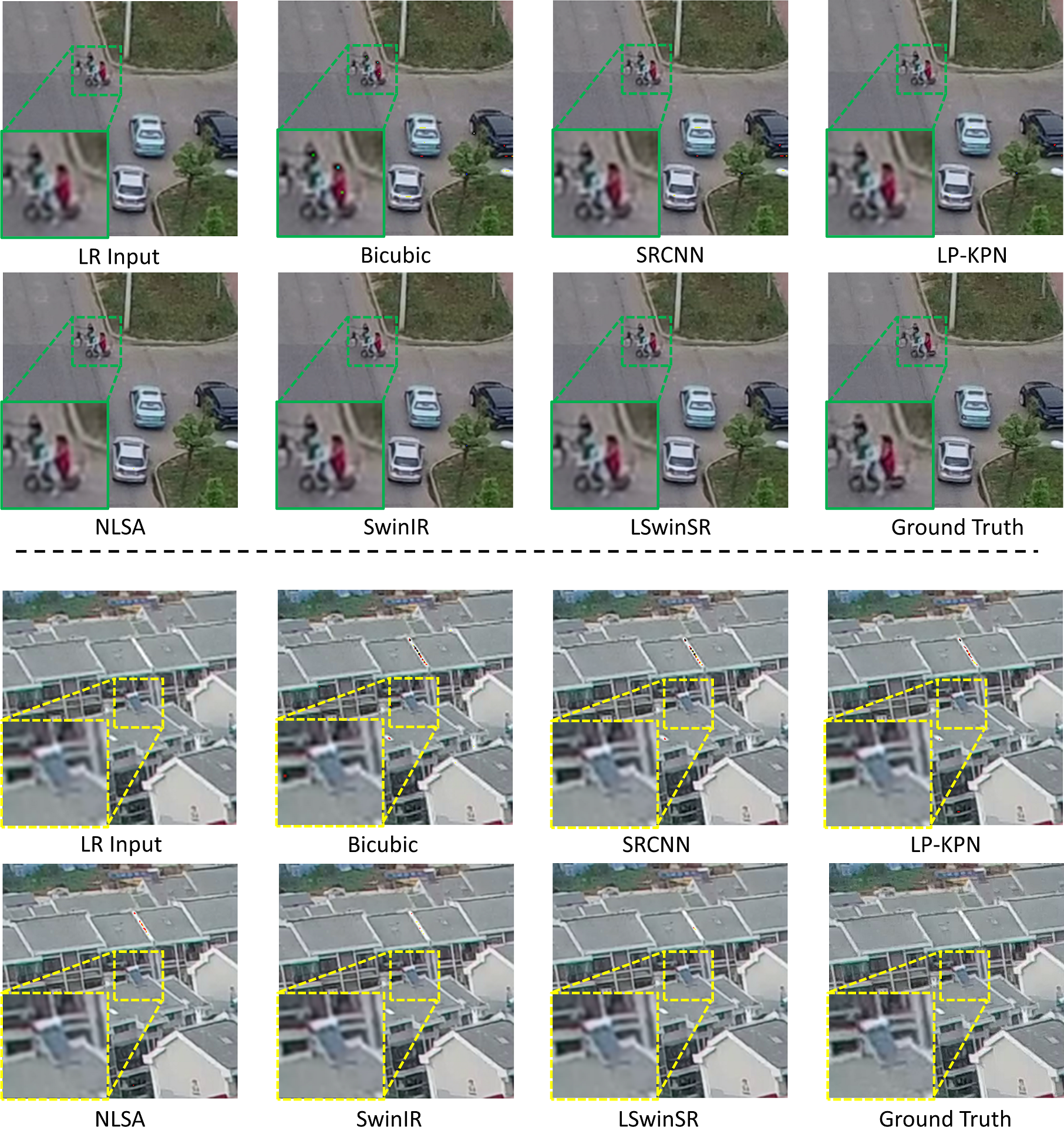
In addition to quantitative results, the qualitative comparison of the reconstructed results with different methods is also provided from Fig. 2 to Fig. 7, where an enlarged region is presented on the corner within each corresponding image for convenient comparison.

Obviously, a better reconstruction can be achieved on the lower super-resolution scale. For example, in Fig. 2, the e-bike riders (top) and the building contours (bottom) generated by different methods are all recognizable. However, the noises of images generated by the Bicubic, SRCNN [6], LP-KPN [35] and NLSA [36] are much clearer and more than those by the SwinIR [28] and the LSwinSR. For example, in the bottom part of Fig. 2, there exist dozens of obvious reddish and blackish noisy points on the white vertical ridge of the building in images predicted by the Bicubic and CNN-based methods. In contrast, for those images generated by Transformer-based methods, the existence of such severe noisy points is much less frequent. Specifically, images predicted by SwinIR [28] and LSwinSR contain only two and one such noisy points, respectively.

With the increase of the upsample scale, the available information for accurate reconstruction becomes more and more scarce, leading to great challenges for super-resolution algorithms. For example, in the top part of Fig. 4, only SwinIR [28] and the proposed LSwinSR provide smooth results for the text in the image when upsampling $\times 4$ scale. By comparison, the image generated by the Bicubic interpolation contains serious noises, while the image predicted by SRCNN [6] is more blurry than others. For LP-KPN [35] and NLSA [36], the problem is the unnecessary wrinkles in the reconstructed texts. When it comes to $\times 8$ super-resolution, the super-resolution algorithms can only rely on very limited input information. As shown in Fig. 7, the details of the building structure are nearly indistinguishable for all methods, but the Transformer-based methods still provide a clearer contour.

4.2.3 Inference Speed

Table 2: The comparison of complexity and inference speed between SwinIR [28] and LSwinSR under different window sizes. The complexity is measured by the Multiply-Accumulate Operations (MACs), while the inference speed, i.e. Frames Per Second (FPS), is evaluated based on the

4\times 3\times 128\times 128

input.

Window Size	Model	Complexity (G) $\downarrow$	Speed $\uparrow$
8	LSwinSR	15.3	14.2
8	SwinIR	16.8	13.5
16	LSwinSR	17.6	12.2
16	SwinIR	25.8	6.9
32	LSwinSR	26.6	6.7
32	SwinIR	62.0	2.1

As the proposed LSwinSR is an improved and simplified version of SwinIR [28], the complexity and the inference speed between the two models are compared. As can be seen in Table 2, the complexity and the inference speed of our LSwinSR are slightly better than SwinIR [28] when the window size is eight. The reason why the gap is so small is two-fold. First, the other operations except for the self-attention mechanism such as patch embedding, patch merging and MLP also occupy a large part of the network structure. Second, the complexity of the traditional self-attention mechanism increases quadratically with the size of the input, while the high computational requirement is not obvious for a small window size. Therefore, the complexity and inference speed gaps between the LSwinSR and SwinIR [28] are dramatically widened with the increase of window sizes. When the window size reaches 32, the inference speed of the LSwinSR is at least three times faster than the SwinIR [28].

Table 3: Quantitative comparison for segmentation based on super-resolution images generated by different methods on the test set. The results based on the original high-resolution images (HR) and the high-resolution image with Gaussian Blur (HR-Blur) are marked in light purple and light blue respectively, while the best result is highlighted and the second best is underlined.

Model	Scale	Clutter	Building	Road	Tree	Vegetation	Static Car	Moving Car	Human	mIoU
Bicubic	$\times 2$	0.592	0.825	0.761	0.749	0.577	0.417	0.661	0.229	0.601
SRCNN [6]	$\times 2$	0.602	0.814	0.766	0.734	0.575	0.360	0.661	0.244	0.595
LP-KPN [35]	$\times 2$	0.596	0.815	0.747	0.756	0.559	0.414	0.658	0.246	0.599
NLSA [36]	$\times 2$	0.599	0.817	0.761	0.754	0.583	0.440	0.656	0.257	0.608
SwinIR [28]	$\times 2$	0.617	0.828	0.771	0.757	0.599	0.441	0.683	0.265	0.620
LSwinSR	$\times 2$	0.605	0.821	0.756	0.774	0.602	0.469	0.686	0.273	0.623
[0.5pt/5pt] HR-Blur	$\times 2$	0.603	0.835	0.745	0.705	0.562	0.476	0.630	0.232	0.599
HR	$\times 2$	0.635	0.850	0.775	0.777	0.593	0.509	0.676	0.273	0.636
Bicubic	$\times 4$	0.594	0.812	0.755	0.757	0.580	0.427	0.648	0.187	0.595
SRCNN [6]	$\times 4$	0.593	0.813	0.743	0.759	0.587	0.392	0.643	0.203	0.592
LP-KPN [35]	$\times 4$	0.603	0.827	0.765	0.759	0.585	0.436	0.653	0.206	0.604
NLSA [36]	$\times 4$	0.585	0.816	0.755	0.759	0.582	0.399	0.645	0.202	0.593
SwinIR [28]	$\times 4$	0.607	0.829	0.768	0.756	0.579	0.483	0.655	0.202	0.610
LSwinSR	$\times 4$	0.603	0.824	0.761	0.757	0.586	0.486	0.657	0.213	0.611
[0.5pt/5pt] HR-Blur	$\times 4$	0.611	0.841	0.758	0.698	0.557	0.532	0.609	0.225	0.604
HR	$\times 4$	0.642	0.850	0.785	0.782	0.601	0.530	0.680	0.270	0.643
Bicubic	$\times 8$	0.553	0.774	0.732	0.726	0.562	0.322	0.588	0.007	0.533
SRCNN [6]	$\times 8$	0.446	0.677	0.640	0.602	0.464	0.036	0.150	0.000	0.377
LP-KPN [35]	$\times 8$	0.565	0.795	0.743	0.735	0.558	0.338	0.611	0.149	0.562
NLSA [36]	$\times 8$	0.572	0.793	0.748	0.730	0.565	0.376	0.611	0.145	0.567
SwinIR [28]	$\times 8$	0.573	0.791	0.751	0.744	0.576	0.330	0.637	0.173	0.572
LSwinSR	$\times 8$	0.590	0.803	0.753	0.748	0.572	0.321	0.640	0.159	0.573
[0.5pt/5pt] HR-Blur	$\times 8$	0.628	0.849	0.776	0.713	0.567	0.535	0.675	0.229	0.621
HR	$\times 8$	0.654	0.856	0.800	0.787	0.615	0.546	0.712	0.292	0.658

4.3 Semantic Segmentation Performance

As the image quality assessments such as PSNR and SSIM cannot directly reflect the reliability of the predicted images for practical applications, we further evaluate the robustness of the reconstructed images from different methods for semantic segmentation.

For each super-resolution method, the UNetFormer [24] is trained and validated using the upsampled training and validation sets for segmentation, whereafter the trained UNetFormer [24] is then used to predict the segmentation maps of the upsampled test set, i.e. the training, validation and test sets are all upsampled by each corresponding super-resolution method. As a reference, we train the model based on the original high-resolution images and report the segmentation accuracy based on the original test set (HR) and the test set after Gaussian Blur (HR-Blur). The visual comparisons between segmentation maps based on super-resolution images generated by different algorithms are provided from Fig. 8 to Fig. 10.

As can be seen from Table 3, due to the different probability distribution between the training set and test set, the accuracy of the test set with Gaussian Blur (HR-Blur) is obviously lower than the original test set (HR). Fortunately, this distributional difference can be offset by the super-resolution methods to a certain degree. For example, as shown in Table 3, the segmentation accuracy of the Bicubic interpolation for $\times 2$ scenario (mIoU: 0.601) is even better than the HR-Blur (mIoU: 0.599). We conjecture that the distributional difference gap between the training set and test set is narrowed after downsampling and upsampling operations, relieving the adverse impact caused by the Gaussian Blur. However, when it comes to the $\times 8$ scale, the accuracy of HR-Blur surpasses all super-resolution methods, even with a different probability distribution with the training set. The reason is that small objects such as humans and cars are hardly identifiable after downsampling to $1/8$ resolution, while such severe information loss cannot be totally recovered by the super-resolution methods. Therefore, the adverse impact caused by information loss overshadows the distributional difference, leading to the worse segmentation accuracy of super-resolution results.

Among five deep-learning-based methods, only the SwinIR [28] and the proposed LSwinSR can always deliver better results than the simple Bicubic interpolation for all three scales, demonstrating the reliability and robustness of the Transformer-based super-resolution methods on different scenarios. Meanwhile, what the segmentation accuracy can show is only the superiority rather than the full potential of the Transformer-based solution. For example, as shown in the enlarged region in Fig. 5, the cyclist can be clearly identified. However, only a small part of those pixels is correctly classified as Human in Fig. 9, even for the original high-resolution input. The reason is that the humans in the UAVid are very small and only occupy limited pixels in the high-resolution 4K images. Without enough training data, the segmentation model naturally lacks the ability to interpret those small objects. Actually, the best accuracy on the Human object for the UAVid dataset achieved by the state-of-the-art segmentation model is only 0.33 measured by mIoU. In other words, the capability of the segmentation model limits the full potential of the super-resolution results in segmentation performance. Thus, with the development of the segmentation model especially the optimization for the identification of small objects, we believe a much better segmentation accuracy can be achieved by the super-resolution results.

It is also noteworthy that the segmentation accuracy of NLSA [36] for $\times 8$ scale (mIoU: 0.567) is much higher than the SRCNN [6] (mIoU: 0.377), although the latter holds better image quality assessments, e.g. the PSNR of SRCNN is 20.000 while the one of the NLAS is 18.453. This phenomenon can illustrate two issues. First, the higher image quality metrics are not always connected with better reliability. Second, even though the over-fitting problem can cause an extremely low image quality assessment, a tolerable segmentation result can still be guaranteed so long as the model can narrow the probability distribution gap between the training set and test set.

5 Conclusions

In this work, a novel Linear Swin Transformer for Super-Resolution (LSwinSR) was proposed. The LSwinSR has addressed the high memory and computational requirements of the original Swin Transformer caused by the quadratic complexity of the embedded self-attention mechanism by introducing the kernel attention mechanism. The super-resolution experiments conducted on the large-scale UAVid dataset demonstrated that the proposed LSwinSR could provide competitive performance compared to the SwinIR [28] but with better efficiency. Furthermore, the experiments for semantic segmentation demonstrated that the super-resolution technology could indeed enhance the segmentation accuracy, where only two Transformer-based super-resolution methods could always deliver better performance than the simple Bicubic interpolation.

In the future, we will investigate the potential solution to integrate the super-resolution models and semantic segmentation models, thereby providing more accurate and reliable segmentation results based on super-resolution technology.

Declaration of Competing Interest

The authors declare that they have no known competing financial interests or personal relationships that could have appeared to influence the work reported in this paper.

CRediT authorship contribution statement

Rui Li: Formal analysis, Conceptualization, Investigation, Methodology, Project administration, Software, Validation, Visualization, Writing - original draft. Xiaowei Zhao: Conceptualization, Formal analysis, Investigation, Methodology, Project administration, Resources, Supervision, Writing - review and editing.

Acknowledgements

The authors acknowledge the support of the Scientific Computing Research Technology Platform (SCRTP) at the University of Warwick for providing High-Performance Computing resources.

Appendix 0.A Super-resolution performance on AID

To further demonstrate the effectiveness of the proposed LSwinSR, we conduct the experiment on the publicly available AID [47] dataset, which has been used for verifying the super-resolution performance. The AID dataset contains 10000 high-resolution images in the shape of $600\times 600$ with a 0.5m spatial resolution from 30 different types of remote sensing scenarios, such as airports, bridges and churches. For super-resolution, 7850 images are selected as the training set, 150 as the validation set and the remaining 2000 images are used as the test set. The experimental results are reported in Table A1. As shown in Table A1, in the large-scale and high-resolution remote sensing dataset, i.e. the AID [47], the proposed LSwinSR can still deliver competitive accuracy compared with the existing super-resolution algorithms.

Table A1: Quantitative comparison including PSNR and SSIM (%) with different methods on the AID dataset, where the best result is highlighted while the second best is underlined.

Model	Scale	PSNR $\uparrow$	SSIM $\uparrow$
Bicubic	$\times 2$	32.39	89.06
SRCNN [6]	$\times 2$	34.49	92.86
FSRCNN [30]	$\times 2$	34.73	93.30
VDSR [29]	$\times 2$	35.05	93.46
LGCNet [48]	$\times 2$	34.80	93.20
DCM [49]	$\times 2$	35.21	93.66
HSENet [50]	$\times 2$	35.24	93.68
LSwinSR	$\times 2$	35.29	93.75
Bicubic	$\times 3$	29.08	78.63
SRCNN [6]	$\times 3$	30.55	83.72
FSRCNN [30]	$\times 3$	30.98	84.00
VDSR [29]	$\times 3$	31.15	85.22
LGCNet [48]	$\times 3$	30.73	84.17
DCM [49]	$\times 3$	31.31	85.61
HSENet [50]	$\times 3$	31.39	85.72
LSwinSR	$\times 3$	31.41	85.83
Bicubic	$\times 4$	27.30	70.36
SRCNN [6]	$\times 4$	28.40	75.61
FSRCNN [30]	$\times 4$	28.77	77.20
VDSR [29]	$\times 4$	28.99	77.53
LGCNet [48]	$\times 4$	28.61	76.26
DCM [49]	$\times 4$	29.17	78.24
HSENet [50]	$\times 4$	29.21	78.50
LSwinSR	$\times 4$	29.23	78.52

References

[1] Q. Zhang, S. Zheng, C. Zhang, X. Wang, R. Li, Efficient large-scale oblique image matching based on cascade hashing and match data scheduling, Pattern Recognition 138 (2023) 109442.
[2] H. Yuan, C. Xiao, Y. Wang, X. Peng, Y. Wen, Q. Li, Maritime vessel emission monitoring by an uav gas sensor system, Ocean Engineering 218 (2020) 108206.
[3] S. Hu, W. Ni, X. Wang, A. Jamalipour, D. Ta, Joint optimization of trajectory, propulsion, and thrust powers for covert uav-on-uav video tracking and surveillance, IEEE Transactions on Information Forensics and Security 16 (2020) 1959–1972.
[4] J. Xie, L. Fang, B. Zhang, J. Chanussot, S. Li, Super resolution guided deep network for land cover classification from remote sensing images, IEEE Transactions on Geoscience and Remote Sensing 60 (2021) 1–12.
[5] P. Mao, J. Ding, B. Jiang, L. Qin, G. Y. Qiu, How can uav bridge the gap between ground and satellite observations for quantifying the biomass of desert shrub community?, ISPRS Journal of Photogrammetry and Remote Sensing 192 (2022) 361–376.
[6] C. Dong, C. C. Loy, K. He, X. Tang, Image super-resolution using deep convolutional networks, IEEE transactions on pattern analysis and machine intelligence 38 (2) (2015) 295–307.
[7] Z. Lu, J. Li, H. Liu, C. Huang, L. Zhang, T. Zeng, Transformer for single image super-resolution, in: Proceedings of the IEEE/CVF Conference on Computer Vision and Pattern Recognition, 2022, pp. 457–466.
[8] W. Zhang, Y. Liu, C. Dong, Y. Qiao, Ranksrgan: Super resolution generative adversarial networks with learning to rank, IEEE Transactions on Pattern Analysis and Machine Intelligence 44 (10) (2021) 7149–7166.
[9] Z. Chen, X. Guo, P. Y. Woo, Y. Yuan, Super-resolution enhanced medical image diagnosis with sample affinity interaction, IEEE Transactions on Medical Imaging 40 (5) (2021) 1377–1389.
[10] F. A. Dharejo, M. Zawish, F. Deeba, Y. Zhou, K. Dev, S. A. Khowaja, N. M. F. Qureshi, Multimodal-boost: Multimodal medical image super-resolution using multi-attention network with wavelet transform, IEEE/ACM Transactions on Computational Biology and Bioinformatics.
[11] M. T. Razzak, G. Mateo-García, G. Lecuyer, L. Gómez-Chova, Y. Gal, F. Kalaitzis, Multi-spectral multi-image super-resolution of sentinel-2 with radiometric consistency losses and its effect on building delineation, ISPRS Journal of Photogrammetry and Remote Sensing 195 (2023) 1–13.
[12] V. Vasilescu, M. Datcu, D. Faur, A cnn-based sentinel-2 image super-resolution method using multiobjective training, IEEE Transactions on Geoscience and Remote Sensing 61 (2023) 1–14.
[13] J. Wang, Z. Shao, X. Huang, T. Lu, R. Zhang, Y. Li, From artifact removal to super-resolution, IEEE Transactions on Geoscience and Remote Sensing 60 (2022) 1–15.
[14] C. Xiang, W. Wang, L. Deng, P. Shi, X. Kong, Crack detection algorithm for concrete structures based on super-resolution reconstruction and segmentation network, Automation in Construction 140 (2022) 104346.
[15] J. Jiang, J. Liu, J. Fu, W. Wang, H. Lu, Super-resolution semantic segmentation with relation calibrating network, Pattern Recognition 124 (2022) 108501.
[16] X. Wang, K. Yu, S. Wu, J. Gu, Y. Liu, C. Dong, Y. Qiao, C. Change Loy, Esrgan: Enhanced super-resolution generative adversarial networks, in: Proceedings of the European conference on computer vision (ECCV) workshops, 2018, pp. 0–0.
[17] Z. Li, J. Yang, Z. Liu, X. Yang, G. Jeon, W. Wu, Feedback network for image super-resolution, in: Proceedings of the IEEE/CVF conference on computer vision and pattern recognition, 2019, pp. 3867–3876.
[18] M. V. Conde, U.-J. Choi, M. Burchi, R. Timofte, Swin2sr: Swinv2 transformer for compressed image super-resolution and restoration, in: Computer Vision–ECCV 2022 Workshops: Tel Aviv, Israel, October 23–27, 2022, Proceedings, Part II, Springer, 2023, pp. 669–687.
[19] A. Vaswani, N. Shazeer, N. Parmar, J. Uszkoreit, L. Jones, A. N. Gomez, L. u. Kaiser, I. Polosukhin, Attention is all you need, in: Advances in Neural Information Processing Systems, Vol. 30, 2017.
[20] A. Dosovitskiy, L. Beyer, A. Kolesnikov, D. Weissenborn, X. Zhai, T. Unterthiner, M. Dehghani, M. Minderer, G. Heigold, S. Gelly, et al., An image is worth 16x16 words: Transformers for image recognition at scale, in: International Conference on Learning Representations, 2021.
[21] Z. Liu, Y. Lin, Y. Cao, H. Hu, Y. Wei, Z. Zhang, S. Lin, B. Guo, Swin transformer: Hierarchical vision transformer using shifted windows, in: Proceedings of the IEEE/CVF international conference on computer vision, 2021, pp. 10012–10022.
[22] X. Zhu, W. Su, L. Lu, B. Li, X. Wang, J. Dai, Deformable detr: Deformable transformers for end-to-end object detection, in: International Conference on Learning Representations, 2021.
[23] Z. Liu, H. Hu, Y. Lin, Z. Yao, Z. Xie, Y. Wei, J. Ning, Y. Cao, Z. Zhang, L. Dong, et al., Swin transformer v2: Scaling up capacity and resolution, in: Proceedings of the IEEE/CVF conference on computer vision and pattern recognition, 2022, pp. 12009–12019.
[24] L. Wang, R. Li, C. Zhang, S. Fang, C. Duan, X. Meng, P. M. Atkinson, Unetformer: A unet-like transformer for efficient semantic segmentation of remote sensing urban scene imagery, ISPRS Journal of Photogrammetry and Remote Sensing 190 (2022) 196–214.
[25] R. Li, S. Zheng, C. Zhang, C. Duan, J. Su, L. Wang, P. M. Atkinson, Multiattention network for semantic segmentation of fine-resolution remote sensing images, IEEE Transactions on Geoscience and Remote Sensing 60 (2021) 1–13.
[26] R. Li, S. Zheng, C. Duan, J. Su, C. Zhang, Multistage attention resu-net for semantic segmentation of fine-resolution remote sensing images, IEEE Geoscience and Remote Sensing Letters 19 (2021) 1–5.
[27] R. Li, S. Zheng, C. Zhang, C. Duan, L. Wang, P. M. Atkinson, Abcnet: Attentive bilateral contextual network for efficient semantic segmentation of fine-resolution remotely sensed imagery, ISPRS Journal of Photogrammetry and Remote Sensing 181 (2021) 84–98.
[28] J. Liang, J. Cao, G. Sun, K. Zhang, L. Van Gool, R. Timofte, Swinir: Image restoration using swin transformer, in: Proceedings of the IEEE/CVF international conference on computer vision, 2021, pp. 1833–1844.
[29] J. Kim, J. K. Lee, K. M. Lee, Accurate image super-resolution using very deep convolutional networks, in: Proceedings of the IEEE conference on computer vision and pattern recognition, 2016, pp. 1646–1654.
[30] C. Dong, C. C. Loy, X. Tang, Accelerating the super-resolution convolutional neural network, in: Computer Vision–ECCV 2016: 14th European Conference, Amsterdam, The Netherlands, October 11-14, 2016, Proceedings, Part II 14, Springer, 2016, pp. 391–407.
[31] M. S. Sajjadi, B. Scholkopf, M. Hirsch, Enhancenet: Single image super-resolution through automated texture synthesis, in: Proceedings of the IEEE international conference on computer vision, 2017, pp. 4491–4500.
[32] K. He, X. Zhang, S. Ren, J. Sun, Deep residual learning for image recognition, in: Proceedings of the IEEE conference on computer vision and pattern recognition, 2016, pp. 770–778.
[33] C. Ledig, L. Theis, F. Huszár, J. Caballero, A. Cunningham, A. Acosta, A. Aitken, A. Tejani, J. Totz, Z. Wang, et al., Photo-realistic single image super-resolution using a generative adversarial network, in: Proceedings of the IEEE conference on computer vision and pattern recognition, 2017, pp. 4681–4690.
[34] B. Lim, S. Son, H. Kim, S. Nah, K. Mu Lee, Enhanced deep residual networks for single image super-resolution, in: Proceedings of the IEEE conference on computer vision and pattern recognition workshops, 2017, pp. 136–144.
[35] J. Cai, H. Zeng, H. Yong, Z. Cao, L. Zhang, Toward real-world single image super-resolution: A new benchmark and a new model, in: Proceedings of the IEEE/CVF International Conference on Computer Vision, 2019, pp. 3086–3095.
[36] Y. Mei, Y. Fan, Y. Zhou, Image super-resolution with non-local sparse attention, in: Proceedings of the IEEE/CVF Conference on Computer Vision and Pattern Recognition, 2021, pp. 3517–3526.
[37] OpenAI, Gpt-4 technical report, 2023.
[38] L. Wang, S. Fang, X. Meng, R. Li, Building extraction with vision transformer, IEEE Transactions on Geoscience and Remote Sensing 60 (2022) 1–11.
[39] R. Strudel, R. Garcia, I. Laptev, C. Schmid, Segmenter: Transformer for semantic segmentation, in: Proceedings of the IEEE/CVF international conference on computer vision, 2021, pp. 7262–7272.
[40] L. Wang, R. Li, C. Duan, C. Zhang, X. Meng, S. Fang, A novel transformer based semantic segmentation scheme for fine-resolution remote sensing images, IEEE Geoscience and Remote Sensing Letters 19 (2022) 1–5.
[41] F. Yang, H. Yang, J. Fu, H. Lu, B. Guo, Learning texture transformer network for image super-resolution, in: Proceedings of the IEEE/CVF conference on computer vision and pattern recognition, 2020, pp. 5791–5800.
[42] S. Lei, Z. Shi, W. Mo, Transformer-based multistage enhancement for remote sensing image super-resolution, IEEE Transactions on Geoscience and Remote Sensing 60 (2021) 1–11.
[43] Y.-H. H. Tsai, S. Bai, M. Yamada, L.-P. Morency, R. Salakhutdinov, Transformer dissection: An unified understanding for transformer’s attention via the lens of kernel, in: Proceedings of the Conference on Empirical Methods in Natural Language Processing, 2019.
[44] T. Xiao, M. Singh, E. Mintun, T. Darrell, P. Dollár, R. Girshick, Early convolutions help transformers see better, Advances in Neural Information Processing Systems 34 (2021) 30392–30400.
[45] Y. Lyu, G. Vosselman, G.-S. Xia, A. Yilmaz, M. Y. Yang, Uavid: A semantic segmentation dataset for uav imagery, ISPRS journal of photogrammetry and remote sensing 165 (2020) 108–119.
[46] G. Bradski, The OpenCV Library, Dr. Dobb’s Journal of Software Tools.
[47] G.-S. Xia, J. Hu, F. Hu, B. Shi, X. Bai, Y. Zhong, L. Zhang, X. Lu, Aid: A benchmark data set for performance evaluation of aerial scene classification, IEEE Transactions on Geoscience and Remote Sensing 55 (7) (2017) 3965–3981.
[48] S. Lei, Z. Shi, Z. Zou, Super-resolution for remote sensing images via local–global combined network, IEEE Geoscience and Remote Sensing Letters 14 (8) (2017) 1243–1247.
[49] J. M. Haut, M. E. Paoletti, R. Fernández-Beltran, J. Plaza, A. Plaza, J. Li, Remote sensing single-image superresolution based on a deep compendium model, IEEE Geoscience and Remote Sensing Letters 16 (9) (2019) 1432–1436.
[50] S. Lei, Z. Shi, Hybrid-scale self-similarity exploitation for remote sensing image super-resolution, IEEE Transactions on Geoscience and Remote Sensing 60 (2021) 1–10.