A statistical framework for GWAS of high dimensional phenotypes using summary statistics, with application to metabolite GWAS

For $\bm{Z}\in\mathbb{R}^{n\times m}$, we let $\bm{Z}_{i*}\in\mathbb{R}^{m}$, $\bm{Z}_{*j}\in\mathbb{R}^{n}$, and $\bm{Z}_{ij}\in\mathbb{R}$ be the $i$th row, $j$th column, and $(i,j)$th element of $\bm{Z}$. We use standard matrix normal notation, i.e. for $\bm{M}\in\mathbb{R}^{n\times m}$, $\bm{U}\in\mathbb{R}^{n\times n}$, and $\bm{V}\in\mathbb{R}^{m\times m}$, $\bm{Z}\sim MN(\bm{M},\bm{U},\bm{V})$ if $\mvec(\bm{Z})\sim N(\mvec(\bm{M}),\bm{V}\otimes\bm{U})$. Vector $\bm{x}\sim(\bm{\mu},\bm{A})$ if $\mathbb{E}(\bm{x})=\bm{\mu}$ and $\V(\bm{x})=\bm{A}$.

Let $\bm{Y}\in\mathbb{R}^{N\times M}$ be the unobserved levels of $M$ phenotypes (metabolites) measured in $N$ unrelated individuals and $\bm{X}\in\mathbb{R}^{N\times S}$ be the unobserved genotypes at $S$ SNPs in the same individuals. Assume

The mean 0 and independence assumption are equivalent to mean-centering $\bm{X}$’s columns and pruning SNPs for linkage disequilibrium, where pruning helps avoid inferring redundant genetic effects. Figure 1 provides a graphical description of our model for the effect of genotypes on phenotypes, which decomposes the total effect into a direct effect and an indirect effect mediated by $K$ latent factors $\bm{C}\in\mathbb{R}^{N\times K}$, and is equivalent to the following model:

where $\bm{L}_{mk}$ is the effect of the $k$th latent factor on the $m$th phenotype and $\bm{G}_{sk}$ is the effect of the $s$th SNP on the $k$th factor. Under this model, $\bm{G}$, $\bm{L}$, and $\bm{\Delta}$ are the parameters of interest and $\mathbb{E}(\bm{Y}\mid\bm{X},\bm{G},\bm{L},\bm{\Delta})=\bm{X}(\bm{G}\bm{L}^{\top}+\bm{\Delta})$ is the total genetic effect, where $\bm{G}_{s*}^{\top}\bm{L}_{m*}$ and $\bm{\Delta}_{sm}$ are the indirect and direct effects of the $s$th SNP on the $m$th phenotype. The non-genetic covariance between phenotypes $\V(\bm{Y}_{i*}\mid\bm{X},\bm{G},\bm{L},\bm{\Delta})=\bm{L}\bm{\Psi}\bm{L}^{\top}+\diag(\sigma_{1}^{2},\ldots,\sigma_{M}^{2})$ is low rank plus diagonal, which is a standard assumption in metabolite, microbiome, and other multi-phenotype data (Sankaran & Holmes 2018; McKennan et al. 2020; Tanigawa et al. 2019). Since we propose a Bayesian method to infer $\bm{G}$, $\bm{L}$, and $\bm{\Delta}$, we explicitly condition on them in the above and below probability statements to avoid confusion.

Two features of (2.1) help motivate assumptions on $\bm{G}$ and $\bm{\Delta}$. First, the first term in the total genetic coefficient $\bm{G}\bm{L}^{\top}+\bm{\Delta}$ captures patterns of inter-phenotype and inter-SNP effect sharing, suggesting $\bm{\Delta}$ should reflect idiosyncratic genetic variation. Second, both $\bm{G}$ and $\bm{\Delta}$ represent direct effects of genotype on a set of phenotypes, and are consequently expected to be sparse with small non-zero entries (Zhang et al. 2018). We therefore assume throughout that

$\bm{\Delta}$’s entry-wise independence implies it captures idiosyncratic genetic variation which, along with its entries’ symmetric spike and slab distributions, are classic assumptions on genetic effects in GWAS with one and more than one phenotype (Zhou et al. 2013; Zhu & Stephens 2017; Ruffieux et al. 2017; Zhang et al. 2018; Turley et al. 2018; Majumdar et al. 2018). The mixture-normal slab is quite general and can approximate a large class of symmetric distributions (Stephens 2017). The parameters $\tau_{sma}$ determine the magnitude of $\bm{\Delta}$’s non-zero effects, where the conditions on $N^{1/2}\tau_{sma}$ and $N^{1/2}\bm{G}_{s*}$ reflect the observation that GWAS z-scores, whose magnitudes scale with $N^{1/2}$ times the SNPs’ effect sizes, are typically small to moderate in real data (Zhu & Stephens 2017; Zhang et al. 2018). Sparsity is implied by our condition on $\pi_{sm}$ in (a) and the sum of squares constraint in (b). It is important to note that while we assume $\bm{\Delta}$ is random, weak convergence results for all frequentist estimators in Section 3.4 are stated conditional on $\bm{\Delta}$. Assuming $\bm{\Delta}$ is random can be thought of as a way to only consider $\bm{\Delta}$’s likely to arise in genetic data and ignore unrealistic “corner cases”. We discuss assumptions for (2.1)’s remaining parameters in Section 3.4.

We assume the GWAS summary statistics $\hat{\beta}_{sm}=(\bm{X}_{*s}^{\top}\bm{X}_{*s})^{-1}\bm{X}_{*s}^{\top}\bm{Y}_{*m}$ from the regressions of the $m$th phenotype onto $s$th SNP’s genotype are observed by the user. We also assume $\bm{X}_{*s}^{\top}\bm{X}_{*s}$ is known, although this can be estimated from public data if unavailable (Auton et al. 2015). We define the observable matrix of standardized GWAS statistics $\hat{\bm{B}}\in\mathbb{R}^{S\times M}$ to be $\hat{\bm{B}}_{sm}=(\bm{X}_{*s}^{\top}\bm{X}_{*s})^{1/2}\hat{\beta}_{sm}$ which, for $\bm{D}=\diag\{(\bm{X}_{*1}^{\top}\bm{X}_{*1}),\ldots,(\bm{X}_{*S}^{\top}\bm{X}_{*S})\}$ and $\bm{R}=\bm{D}^{-1/2}\bm{X}^{\top}\bm{X}\bm{D}^{-1/2}$ (the in-sample correlation between SNPs), can be expressed as

Standardizing summary statistics by $(\bm{X}_{*s}^{\top}\bm{X}_{*s})^{1/2}$ is akin to working with z-scores and begets rows (SNPs) with identical covariances, where $\bm{D}^{1/2}\bm{G}$ and $\bm{D}^{1/2}\bm{\Delta}$ are the standardized analogues of $\bm{G}$ and $\bm{\Delta}$. Although the diagonal elements of $\bm{D}$ grow with the sample size, Assumption 2.2 implies $\bm{D}^{1/2}\bm{G}$ and $\bm{D}^{1/2}\bm{\Delta}$ are moderate. Evidently, $\hat{\bm{B}}$ depends on $\bm{D}^{1/2}\bm{G}$ and $\bm{D}^{1/2}\bm{\Delta}$ through $\bm{R}(\bm{D}^{1/2}\bm{G})$ and $\bm{R}(\bm{D}^{1/2}\bm{\Delta})$. However, since the off-diagonal elements of $\bm{R}$ are small under Assumption 2.1, the sparsity assumptions in Assumption 2.2 imply $\bm{R}(\bm{D}^{1/2}\bm{G})\approx\bm{D}^{1/2}\bm{G}$ and $\bm{R}(\bm{D}^{1/2}\bm{\Delta})\approx\bm{D}^{1/2}\bm{\Delta}$.

The parameters of interest $(\bm{G},\bm{L})$ in (2.2) are not identifiable, since $(\bm{G}\bm{A},\bm{L}\bm{A}^{-\top})$ will give an identical likelihood for any invertible $K\times K$ matrix $\bm{A}$. We address this with the following proposition.

We use the parametrization in (i) for the remainder of the manuscript, which is a classic way to identify components of factor models (McKennan & Nicolae 2019). The orthogonality of the columns of $\tilde{\bm{G}}$ and $\bm{L}$ also help motivate Algorithm 1 below, which uses singular value decomposition to derive estimates for $\bm{G}$, $\bm{L}$, and $\bm{\Delta}$. Part (ii) of Proposition 2.1 suggests that regardless of parametrization, $\tilde{\bm{G}}$ will never be sparse even if $\bm{G}$ is sparse. This follows because $\tilde{\bm{G}}$ in (2.2) is a noisy version of $\bm{G}$, whose error $\bm{D}^{-1/2}\bm{X}^{\top}\bm{\Xi}$ is dense. This is in stark contrast with existing methods that assume a sparse low rank structure on $\hat{\bm{B}}$ (Petti et al. 2022), suggesting they enforce non-existent sparsity.

Here we present a Bayesian method we call HiGSS (High Dimensional GWAS with Summary Statistics) in Algorithm 1 below to derive the posterior $\Bprob(\bm{G},\bm{L},\bm{\Delta}\mid\hat{\bm{B}},\bm{D})$ assuming the number of latent factors $K$ is known. To circumvent the computational and statistical issues that arise in Bayesian factor analysis, and as alluded to by Proposition 2.1, HiGSS first uses singular value decomposition to derive frequentist estimates for the parameters of interest and subsequently leverages the asymptotic theory developed Section 3.4 to calculate the posterior. HiGSS assumes the priors on $\bm{G}$, $\bm{L}$, and $\bm{\Delta}$ are independent.

The intuition for step 1 is if $\bm{\Delta}$ is sparse, (2.2) and the accuracy of singular value decomposition suggest $\hat{\bm{G}}\approx\tilde{\bm{G}}$, $\hat{\bm{L}}\approx\bm{L}$, and the residuals $\hat{\bm{\Delta}}$ should be approximately $\bm{D}^{1/2}\bm{\Delta}$ plus independent noise (McKennan & Nicolae 2019). The subscripts “$s$” and “$m$” in $\bm{G}$’s and $\bm{L}$’s prior distributions indicate these priors may depend on SNP $s$- and phenotype $m$-specific parameters, and we justify the likelihoods for $\hat{\bm{G}}$, $\hat{\bm{L}}$, and $\hat{\bm{\Delta}}$ from steps 2-4 in Section 3.4. Since $\bm{\Delta}$ contains $S\times M\gtrsim 10^{8}$ elements, computing its posterior is intractable unless an appropriate prior is chosen. The spike and mixture-normal slab prior in step 4, whose parameters’ definitions match those in Assumption 2.2, is conjugate and begets tractable computation. Its concordance with Assumption 2.2 is coincidental and is chosen to match the prevailing choices of priors in GWAS (Zhang et al. 2018).

Step 5 assumes the total posterior $\Bprob(\bm{G},\bm{L},\bm{\Delta}\mid\hat{\bm{B}},\bm{D})$ can be factored into the product of posteriors defined in the previous three steps. To see why this is appropriate, note $\{\hat{\bm{G}},\hat{\bm{L}},\hat{\bm{\Delta}}\}$ is a function of $\hat{\bm{B}}$ and $\hat{\bm{B}}=\hat{\bm{G}}\hat{\bm{L}}^{\top}+\hat{\bm{\Delta}}$, meaning the total posterior is equivalent to

Step 5 therefore follows provided $\hat{\bm{G}}$, $\hat{\bm{L}}$, and $\hat{\bm{\Delta}}$ are independent conditional on $\{\bm{G},\bm{L},\bm{\Delta},\bm{D}\}$, which we prove is true asymptotically in Section 3.4.

Perhaps the most unexpected component of Algorithm 1 is $\hat{\bm{L}}$’s likelihood in step 3. Since $\hat{\bm{B}}$ has $S$ rows, existing singular value decomposition results suggest $\hat{\bm{L}}_{m*}$’s asymptotic variance should be $S^{-1}\hat{\sigma}_{m}^{2}I_{K}$ because $\hat{\bm{L}}_{m*}$ is ostensibly estimated on $S$ degrees of freedom (McKennan & Nicolae 2019). This is quite different from the variance in step 3 which, because $N$ is typically smaller than $S$, is closer to $N^{-1}\hat{\sigma}_{m}^{2}I_{K}$ than $S^{-1}\hat{\sigma}_{m}^{2}I_{K}$. This is sensible because $\hat{\bm{B}}$ in (2.2) is obtained by projecting the $N$ samples up to the space of $S$ SNPs, implying $\hat{\bm{L}}_{m*}$ is actually estimated on something closer to $N$ degrees of freedom. Theorem 3.2 and Corollary 3.1 in Section 3.4 below, which prove the veracity of $\hat{\bm{L}}$’s likelihood, are to our knowledge the first results of their kind and, as we show in Section 5, are critical to the fidelity of inference on $\bm{L}$.

Algorithm 1 is general in that the likelihoods in steps 2-4 and form for the posterior in step 5 are the same regardless of the phenotypes being analyzed. However, the choice of priors will likely depend on the type of phenotypes. For example, the set of priors chosen in metabolomic applications may be different that those in microbiome data. We therefore provide general recommendations for how to choose priors for $\bm{G}$ and $\bm{L}$ and $\bm{\Delta}$’s hyperparameters in Section 3.2.

First, recall $\bm{G}$ is the effect of genotype on a small number ($K$) of latent phenotypes. Since $\hat{\bm{G}}$’s likelihood is normal in Algorithm 1, we can either treat $\bm{G}$’s $K$ columns as independent and use the many single-phenotype GWAS priors designed for and normal data (e.g. Zhu & Stephens 2017 and Zhang et al. 2018), or model $\bm{G}$’s columns dependencies using recent methods designed multi-phenotype GWAS (Turley et al. 2018; Majumdar et al. 2018). We take the former approach in our metabolomic application.

The likelihoods for $\hat{\bm{L}}$ and $\hat{\bm{\Delta}}$ in Algorithm 1 suggest the simplest approach would be to treat estimating $\bm{L}$ and $\bm{\Delta}$ as a normal means problem and use empirical Bayes to derive column-specific and matrix-wide priors, respectively, which can be done efficiently using Stephens 2017. An alternative would be to incorporate prior knowledge on the relationships between the $M$ phenotypes into the prior on $\bm{L}$ and $\bm{\Delta}$’s hyperparameters. For example, it is straightforward to incorporate phylogenetics in $\bm{L}$’s prior using the methods discussed in Zhang et al. 2021, and we show in Section 4 how to leverage metabolic pathways in our prior on $\bm{L}$ and $\bm{\Delta}$’s hyperparameters.

The likelihoods for $\hat{\bm{G}}$ and $\hat{\bm{L}}$ in Algorithm 1 can be written as a product of likelihoods across their $K$ columns. Consequently, provided their priors also factor across their columns, posterior computation on $\bm{G}$ and $\bm{L}$ can be done in parallel across their columns, which is not true for traditional Bayesian or recent empirical Bayes-based factor analysis methods (Zhong et al. 2020; Wang & Stephens 2021).

Estimating $K$ is critical, since underestimating it can cause one to miss important genetic variation and overestimating it by too much can invalidate statistical guarantees. Given $\hat{\bm{B}}$’s model in (2.2), it is tempting to reason that because the off-diagonals of $\bm{R}$ (the in-sample correlation between SNPs) are approximately zero, one can treat the entries of the error matrix $\tilde{\bm{E}}$ as independent and use one of the many estimators designed for omic data with independent errors (Owen & Wang 2016; Dobriban & Owen 2018; Dobriban 2020; Ke et al. 2021). Unfortunately, as shown in Section 5, ignoring the dependencies produced by $\bm{R}$’s off-diagonal elements causes these methods to fail.

One way to address the abovementioned issues could be to use McKennan & Nicolae 2022, which explicitly models the dependence. However, applying their method in this setting would require knowing $\bm{R}$, which is unobservable. A second option might be to use methods whose theoretical results allow $\tilde{\bm{E}}$’s entries be dependent, such as Bai & Ng 2002, Ahn & Horenstein 2013, or Onatski 2010. However, the former two require factor loadings be unrealistically large (i.e. satisfy the pervasive factor assumption) and the latter patently fails in simulated and real omic data (McKennan 2020). To address these deficiencies, note that if we assume for simplicity that $\bm{\Delta}$ in (2.2) is 0,

Consequently, any of $\hat{\bm{B}}$’s singular values that exceed those in a pure noise model must have arisen from the low rank signal. This suggests that if we knew $\tilde{\bm{E}}$’s maximum singular value $s_{\max}$, a natural estimator for $K$ is the number of $\hat{\bm{B}}$’s singular values that exceed $s_{\max}$. We use this reasoning to motivate our novel method dBEMA (dependent Bulk Eigenvalue Matching), which models $\hat{\bm{B}}$’s bulk spectrum to predict $\tilde{\bm{E}}$’s maximum singular value. We describe dBEMA below.

Our method is an extension of Ke et al. 2021 to the setting where $\tilde{\bm{E}}$ has dependent rows. To be consistent with Section 2, we assume throughout that $\bm{E}$ in (2.1), and therefore $\tilde{\bm{E}}$ in (2.2), is Gaussian. However, the universality theory of eigenvalues implied by Onatski 2010 indicates we can relax this to only require $\bm{E}$’s entries satisfy weaker moment conditions.

To motivate the method, suppose $S=S(N)$ and $M=M(N)$ such that $S/N\to\gamma_{S}\in(0,\infty)$ and $M/N\to\gamma_{M}\in(0,\infty)$, and let $F_{R,N}$ and $F_{\sigma^{2},N}$ be the empirical distributions of $\bm{R}$’s $S$ eigenvalues and $\{\sigma_{m}^{2}\}_{m\in[M]}$, respectively. If the distributions $\lim_{N\to\infty}F_{R,N}=F_{R}$ and $\lim_{N\to\infty}F_{\sigma^{2},N}=F_{\sigma^{2}}$ exist and are supported on compact intervals, Lemmas 1 and 3 in Onatski 2010 imply $F_{R}$ and $F_{\sigma^{2}}$ determine the behavior of $\tilde{\bm{E}}$’s bulk and largest singular values. The problem therefore boils down to estimating $F_{R}$ and $F_{\sigma^{2}}$, since this will allow us to predict $\tilde{\bm{E}}$’s maximum singular value.

First, Assumption 2.1 implies $F_{R}$ is exactly the Marchenko–Pastur distribution (Marčenko & Pastur 1967), which for $x\geq 0$, $\lambda_{-}=(1-\sqrt{\gamma_{S}})^{2}$, and $\lambda_{+}=(1+\sqrt{\gamma_{S}})^{2}$ takes the form

Unlike $F_{R}$, $F_{\sigma^{2}}$ is unknown and must be estimated from the data. Following Ke et al. 2021, we model $F_{\sigma^{2}}$ as a gamma distribution and use $\hat{\bm{B}}$’s bulk singular values to estimate its parameters. Briefly, let $\hat{s}_{\min(N,M,S)}\leq\cdots\leq\hat{s}_{1}$ be $\hat{\bm{B}}$’s non-zero singular values and define $\mathcal{B}=\{\hat{s}_{\lfloor(\alpha/2)\min(N,M,S)\rfloor},\ldots,\hat{s}_{\lfloor(1-\alpha/2)\min(N,M,S)\rfloor}\}$ for some $\alpha\in(0,1)$ to be $\hat{\bm{B}}$’s bulk singular values. Since $\mathcal{B}$ excludes $\hat{\bm{B}}$’s $K$ largest singular values for sufficiently large $N$, $\mathcal{B}$’s elements are approximately the inner $1-\alpha$ fraction of $\tilde{\bm{E}}$’s singular values. Consequently, these can be predicted given $F_{R}$ and the rate and scale parameters that parameterize $F_{\sigma^{2}}$. We therefore minimize the difference between $\mathcal{B}$’s elements and their predicted values as a function of the rate and scale parameters to estimate $F_{\sigma^{2}}$. Equipped with $F_{R}$ and an estimate for $F_{\sigma^{2}}$, we lastly determine $\hat{F}_{s_{max}}$, an estimate for the distribution of $\tilde{\bm{E}}$’s maximum singular value, and define our estimate for the number of factors to be the number $\hat{\bm{B}}$’s singular values that exceed the $1-\beta$ quantile of $\hat{F}_{s_{max}}$ for some user-specified $\beta\in(0,1)$. The algorithm is given in Section A1.

As mentioned above, the theoretical work used to motivate dBEMA requires $F_{\sigma^{2}}$ have bounded support, i.e. $\min\{x\in\mathbb{R}\cup\{\infty\}:F_{\sigma^{2}}(x)=1\}<\infty$, which belies our decision to model $F_{\sigma^{2}}$ as a gamma distribution. We use simulated data in Section 5 to show dBEMA performs well despite this.

Here we provide a theoretical justification for the likelihoods for $\hat{\bm{G}}$, $\hat{\bm{L}}$, and $\hat{\bm{\Delta}}$ used in Algorithm 1. Theory for the consistency of our estimate for $K$ proposed in Section 3.3 will appear in a subsequent version of this manuscript. We first present an assumption on the parameters in (2.1).

We assume $N$, $M$, and $S$ are comparable in (a) to be consisted with ‘omic’ and biobank data. The requirement that $\mathbb{E}(S^{-1}\tilde{\bm{G}}^{\top}\tilde{\bm{G}}\mid\bm{G})=I_{K}$ and $M^{-1}\bm{L}^{\top}\bm{L}$ be diagonal with decreasing diagonal elements is without loss of generality by Proposition 2.1, where our condition on the ratio of successive diagonal elements is a standard eigengap assumption and ensures we can identify the columns of $\bm{L}$ and $\bm{G}$ up to sign (McKennan & Nicolae 2019). The parameter $\lambda_{k}$ is the average sum of squares of the $k$th loading $\bm{L}_{*k}$ and is interpretable as the $k$th latent factor’s signal strength, where the “pervasive factor assumption” is satisfied if $\lambda_{1},\ldots,\lambda_{K}\asymp 1$ (Fan et al. 2021). While common in the literature, the pervasive factor assumption is patently violated in ‘omic’ data, where methods that utilize it often cannot recover non-pervasive, but critical, sources of omic variation (McKennan 2020). This is especially important in our data application whose most genetically regulated factors are weaker. We therefore allow $\lambda_{k}$ to be large ($\lambda_{k}\asymp 1$, pervasive) or moderate to small ($\lambda_{k}<<1$, non-pervasive) to ensure we can perform inference on as many types of factors as possible.

We first justify $\hat{\bm{G}}^{\prime}s$ likelihood in step 2 of Algorithm 1. We define $\mathscr{C}_{d}$ and $\Phi_{d}$ to be the set of all convex sets and the distribution function for the standard normal in $\mathbb{R}^{d}$, respectively, for the remainder of the section.

Since the sign multipliers $a_{1},\ldots,a_{K}$ are the same for each SNP $s$, this shows we can estimate each column of $\bm{G}$ up to sign. Theorem 3.1 also justifies treating $\hat{\bm{G}}$’s rows in Algorithm 1 as independent standard normals. We next justify step 3 of Algorithm 1.

Results (i) and (ii) imply $\hat{\sigma}_{m}^{2}$ in step 3 of Algorithm 1 is consistent for $\sigma_{m}^{2}$ and we can infer indirect effects $\bm{G}_{s*}^{\top}\bm{L}_{m*}$. The condition $N^{1/2}\lVert\bm{L}_{m*}\rVert_{2}\to\infty$ will hold if phenotype $m$ is non-trivially affected by at least one latent factor, and appears to be satisfied for nearly all $m$ in our data application. Result (iii) implies $\hat{\bm{L}}_{m*}$ is asymptotically normal with asymptotic variance as given in step 3. However, $\hat{\bm{L}}_{m*}$’s asymptotic distribution is centered around $\bm{A}\bm{L}_{m*}$ rather than $\diag(a_{1},\ldots,a_{K})\bm{L}_{m*}$, which is a standard property of singular value decomposition-based estimates (Wang et al. 2017). Although their difference is small, it may not be small enough to guarantee we can infer $\bm{L}_{m*}$’s sparsity patterns, since $(\bm{A}\bm{L}_{m*})_{k}$ may be larger than its estimate’s standard deviation even if $\bm{L}_{mk}=0$. This is especially important when data contain both pervasive and non-pervasive factors, since $\bm{A}$’s off-diagonal elements risk contaminating sparser, non-pervasive factor loadings with dense pervasive factor loadings. Corollary 3.1 below shows that no such contamination occurs.

The expression for $\bm{A}$ implies we need not worry about the abovementioned contamination, which gives rise to the subsequent result stating the asymptotic distributions for non-pervasive factor loadings are, up to sign, centered around their true loadings. While this is not necessarily true for pervasive factor loadings, it has a negligible effect on inference because contamination will only trivially impact their large non-zero entries and, as illustrated in our data example, pervasive factors are more likely to reflect non-genetic variation. We lastly consider steps 4 and 5 of Algorithm 1.

Part (i) justifies $\hat{\bm{\Delta}}$’s likelihood in Algorithm 1, which assumes its entries are independent and normally distributed. The asymptotic independence of the z-statistics in part (ii), which are the standardized equivalents of $\hat{\bm{G}}$, $\hat{\bm{L}}$, and $\hat{\bm{\Delta}}$, justifies step 5.

Indirect effects of genotype on metabolite levels are parametrized by $\bm{G}$ and $\bm{L}$. Our prior on $\bm{G}$ follows Section 3.2’s discussion and assumes each column’s entries are drawn from a spike and slab:

which is conjugate under $\hat{\bm{G}}$’s normal likelihood in Algorithm 1. Standardizing by $\bm{D}_{ss}$ implies standardized effects $\bm{D}_{ss}^{1/2}\bm{G}_{sk}$ are identically distributed across SNPs $s$ and reflects the observation that genetic effects are typically inversely proportional to minor allele frequency (Park et al. 2011). We estimate $\pi_{G_{k}},\tau_{G_{k}}^{2}$ via empirical Bayes.

Our prior on $\bm{L}$ incorporates metabolic pathway information and is constructed to reflect the following observations from Figure 2(b) and inference goals. First, metabolite loadings from the same sub-pathway appear to be drawn from the same distribution, where sub-pathway distributions within a super-pathway are more similar than those from different super-pathways. Second, Figure 2(b) suggests many sub-pathways have identical loading distributions. For example, the first two orange and green lipid sub-pathways may have the same distributions. Our prior should therefore facilitate a clustering on sub-pathways, which couples biological processes to beget more interpretable inference. Third, it is expected that some metabolites behave as “outliers” because they were incorrectly partitioned or do not follow their sub-pathways’ distributions.

To accommodate these observations, we use a hierarchical Dirichlet process (Teh et al. 2006) to model sub-pathway distribution parameters. This begets a clustering over sub-pathways, where two sub-pathways from the same super-pathway are a priori more likely to lie in the same cluster than sub-pathways from different super-pathways. Metabolite loadings are then either drawn from their sub-pathway’s distribution or, to accommodate the above third observation, an “outlier” distribution. Mathematically, let $p\in[P]$ index super-pathways, $b\in[B_{p}]$ index constituent sub-pathways, and $m\in[M_{pb}]$ index constituent metabolites. We assume $\bm{L}$ has independent columns and, to simplify notation, suppress any dependence on the factor number. As such, we let $\bm{L}_{pbm}\in\mathbb{R}$ be a factor’s loading for the $m$th metabolite in the $b$th and $p$th sub- and super-pathway for the remainder of Section 4.1. Then for concentration parameters $\gamma,\alpha_{0}>0$ and probability measure $H$ on $\mathbb{R}\times\mathbb{R}_{\geq 0}$,

Figure 3(a) provides a graphical description of this prior. Assuming for the moment that $\pi_{\outlier}=0$, $\bm{L}_{pbm}$ is drawn from a hierarchical Dirichlet process mixture model, where mixture components (clusters) are defined by the unique values of $\{(\mu_{pb},\phi^{2}_{pb})\}_{p\in[P];b\in[B_{p}]}$ (Teh et al. 2006). Briefly, the probability measure $F_{0}$ is first drawn from a Dirichlet process with baseline measure $H$ and, with probability one, takes the form $\sum_{j=1}^{\infty}\beta_{0,j}\delta_{(\mu_{j},\phi^{2}_{j})}$ for some probability weights $\beta_{0,j}$ and $(\mu_{j},\phi^{2}_{j})\in\mathbb{R}\times\mathbb{R}_{\geq 0}$. Each $F_{p}$ is subsequently drawn from another Dirichlet process with baseline measure $F_{0}$, meaning $F_{p}$ can also be expressed as $\sum_{j=1}^{\infty}\beta_{p,j}\delta_{(\mu_{j},\phi^{2}_{j})}$ for some probability weights $\beta_{p,j}$. The third line in (4.2) implies sub-pathways within a super-pathway are assigned to clusters based on their parameters $(\mu_{pb},\phi^{2}_{pb})$, where sub-pathways that share parameters fall in the same cluster. However, since the $F_{p}$’s share atoms, sub-pathways from different super-pathways can be assigned to the same cluster, where larger values of $\alpha_{0}$ increase the probability of this occurring.

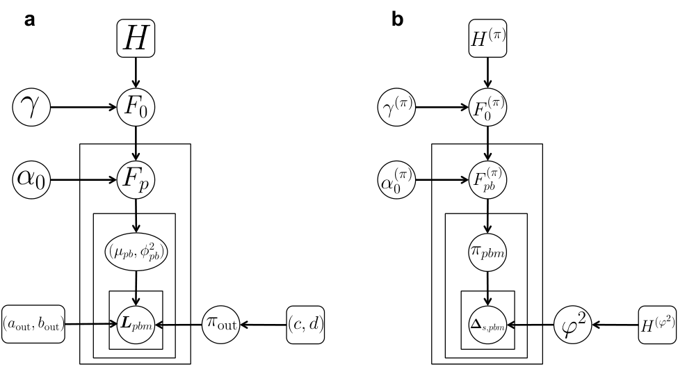
The parameter $\pi_{\outlier}$ in (4.2) is the fraction of all metabolites that are “outliers”, i.e. metabolites whose loadings do not follow the hierarchical Dirichlet process mixture model. Since we assume their loadings can take any value with equal probability, we treat them as uniformly distributed and set $a_{\outlier},b_{\outlier}$ so $[a_{\outlier},b_{\outlier}]$ contains all observed loadings. We let $\pi_{\outlier}\sim\text{Beta}(c,d)$ so as to allow the data to help dictate outlier frequency, and set $c=1/5,d=999/5$ so that out of 1,000 metabolites, we a priori expect one outlier and no more than five outliers with probability 0.95.

Similar to Teh et al. 2006, we place diffuse priors on $\gamma$ and $\alpha_{0}$. We set the base distribution $H$ so that $\mathbb{P}\{(\mu_{pb},\phi_{pb}^{2})=(0,0)\mid H\}>0$ and $\mu_{pb}\perp\!\!\!\perp\phi_{pb}^{2}\mid\{H,(\mu_{pb},\phi_{pb}^{2})\neq(0,0)\}$. The former reflects our belief that some sub-pathways will have loadings exactly equal to 0 and we let $\mu_{pb}\mid\{H,(\mu_{pb},\phi_{pb}^{2})\neq(0,0)\}$ follow a spike and mixture-normal slab to ensure conjugacy, where the slab is chosen to approximate the horseshoe prior (Carvalho et al. 2009). We let $\phi_{pb}^{2}\mid\{H,(\mu_{pb},\phi_{pb}^{2})\neq(0,0)\}$ be a densely discretized gamma distribution, where discretizing facilitates faster computation by letting us to integrate out $\bm{L}$ in our Gibbs sampler. Section A2 provides additional details and describes our Gibbs sampler, which utilizes the Chinese restaurant franchise parametrization of the hierarchical Dirichlet process to efficiently sample from the posterior.

References

- Uffelmann et al. (2021) Emil Uffelmann, Qin Huang, Nchangwi Munung, Jantina de Vries, Yukinori Okada, Alicia. Martin, Hilary. Martin, Tuuli Lappalainen and Danielle Posthuma “Genome-wide association studies” In Nature Reviews Methods Primers 1.1, 2021, pp. 59
- Tanigawa et al. (2019) Yosuke Tanigawa et al. “Components of genetic associations across 2,138 phenotypes in the UK Biobank highlight adipocyte biology” In Nature Communications 10.1, 2019, pp. 4064
- Elliott et al. (2018) Lloyd. Elliott, Kevin Sharp, Fidel Alfaro-Almagro, Sinan Shi, Karla. Miller, Gwenaëlle Douaud, Jonathan Marchini and Stephen. Smith “Genome-wide association studies of brain imaging phenotypes in UK Biobank” In Nature 562.7726, 2018, pp. 210–216
- Yin et al. (2022) Xianyong Yin et al. “Genome-wide association studies of metabolites in Finnish men identify disease-relevant loci” In Nature Communications 13.1, 2022, pp. 1644
- Kurilshikov et al. (2021) Alexander Kurilshikov et al. “Large-scale association analyses identify host factors influencing human gut microbiome composition” In Nature Genetics 53.2, 2021, pp. 156–165
- Yin et al. (2022a) Xianyong Yin et al. “Integrating transcriptomics, metabolomics, and GWAS helps reveal molecular mechanisms for metabolite levels and disease risk” In The American Journal of Human Genetics 109.10 Elsevier BV, 2022, pp. 1727–1741 DOI: 10.1016/j.ajhg.2022.08.007
- Karjalainen et al. (2022) Minna. Karjalainen et al. “Genome-wide characterization of circulating metabolic biomarkers reveals substantial pleiotropy and novel disease pathways” Cold Spring Harbor Laboratory, 2022 DOI: 10.1101/2022.10.20.22281089
- McKennan et al. (2020) Chris McKennan, Carole Ober and Dan Nicolae “Estimation and inference in metabolomics with nonrandom missing data and latent factors” In The Annals of Applied Statistics 14.2, 2020 DOI: 10.1214/20-aoas1328
- Qi & Chatterjee (2018) Guanghao Qi and Nilanjan Chatterjee “Heritability informed power optimization (HIPO) leads to enhanced detection of genetic associations across multiple traits” In PLoS Genetics 14.10, 2018, pp. e1007549
- Dai et al. (2019) Mingwei Dai, Xiang Wan, Hao Peng, Yao Wang, Yue Liu, Jin Liu, Zongben Xu and Can Yang “Joint analysis of individual-level and summary-level GWAS data by leveraging pleiotropy” In Bioinformatics 35.10, 2019, pp. 1729–1736
- Liu et al. (2017) Jin Liu, Xiang Wan, Chaolong Wang, Chao Yang, Xiaowei Zhou and Can Yang “LLR: a latent low-rank approach to colocalizing genetic risk variants in multiple GWAS” In Bioinformatics 33, 2017, pp. 3878–3886
- Lu et al. (2022) Yihao Lu, Meritxell Oliva, Brandon Pierce, Jin Liu and Lin Chen “Integrative cross-omics and cross-context analysis elucidates molecular links underlying genetic effects on complex traits”, 2022 DOI: 10.21203/rs.3.rs-2137179/v1
- Wu (2020) Chong Wu “Multi-trait Genome-Wide Analyses of the Brain Imaging Phenotypes in UK Biobank” In Genetics 215.4 Oxford University Press (OUP), 2020, pp. 947–958 DOI: 10.1534/genetics.120.303242
- Wang et al. (2023) Meida Wang, Xuewei Cao, Shuanglin Zhang and Qiuying Sha “A clustering linear combination method for multiple phenotype association studies based on GWAS summary statistics” In Scientific Reports 13.1, 2023, pp. 3389
- Petti et al. (2022) Samantha Petti, Gautam Reddy and Michael. Desai “Inferring sparse structure in genotype-phenotype maps” In bioRxiv Cold Spring Harbor Laboratory, 2022 DOI: 10.1101/2022.09.27.509675
- Hall et al. (2017) Andrew Hall, Andrew. Tolonen and Ramnik. Xavier “Human genetic variation and the gut microbiome in disease” In Nature Reviews Genetics 18.11, 2017, pp. 690–699
- Zhang et al. (2021) Liangliang Zhang, Yushu Shi, Robert. Jenq, Kim-Anh Do and Christine. Peterson “Bayesian compositional regression with structured priors for microbiome feature selection” In Biometrics 77.3, 2021, pp. 824–838
- Sidén et al. (2017) Per Sidén, Anders Eklund, David Bolin and Mattias Villani “Fast Bayesian whole-brain fMRI analysis with spatial 3D priors” In NeuroImage 146, 2017, pp. 211–225
- Sankaran & Holmes (2018) Kris Sankaran and Susan Holmes “Latent variable modeling for the microbiome” In Biostatistics 20.4, 2018, pp. 599–614 DOI: 10.1093/biostatistics/kxy018
- Zhang et al. (2018) Yan Zhang, Guanghao Qi, Ju-Hyun Park and Nilanjan Chatterjee “Estimation of complex effect-size distributions using summary-level statistics from genome-wide association studies across 32 complex traits” In Nature Genetics 50.9, 2018, pp. 1318–1326
- Zhou et al. (2013) Xiang Zhou, Peter Carbonetto and Matthew Stephens “Polygenic Modeling with Bayesian Sparse Linear Mixed Models” In PLoS Genetics 9.2, 2013, pp. e1003264–
- Zhu & Stephens (2017) Xiang Zhu and Matthew Stephens “Bayesian large-scale multiple regression with summary statistics from genome-wide association studies” In The Annals of Applied Statistics 11.3 NIH Public Access, 2017, pp. 1561
- Ruffieux et al. (2017) Helene Ruffieux, Anthony. Davison, Jorg Hager and Irina Irincheeva “Efficient inference for genetic association studies with multiple outcomes” In Biostatistics 18.4, 2017, pp. 618–636 DOI: 10.1093/biostatistics/kxx007
- Turley et al. (2018) Patrick Turley et al. “Multi-trait analysis of genome-wide association summary statistics using MTAG” In Nature Genetics 50.2, 2018, pp. 229–237
- Majumdar et al. (2018) Arunabha Majumdar, Tanushree Haldar, Sourabh Bhattacharya and John. Witte “An efficient Bayesian meta-analysis approach for studying cross-phenotype genetic associations” In PLoS Genetics 14.2, 2018, pp. e1007139–
- Stephens (2017) Matthew Stephens “False discovery rates: a new deal” In Biostatistics 18.2 Oxford University Press, 2017, pp. 275–294
- Auton et al. (2015) Adam Auton et al. “A global reference for human genetic variation” In Nature 526.7571, 2015, pp. 68–74
- McKennan & Nicolae (2019) Chris McKennan and Dan Nicolae “Accounting for unobserved covariates with varying degrees of estimability in high-dimensional biological data” In Biometrika 106.4, 2019, pp. 823–840 DOI: 10.1093/biomet/asz037
- Zhong et al. (2020) Xinyi Zhong, Chang Su and Zhou Fan “Empirical Bayes PCA in high dimensions” In Journal of the Royal Statistical Society: Series B (Statistical Methodology) 84, 2020, pp. 853–878
- Wang & Stephens (2021) Wei Wang and Matthew Stephens “Empirical Bayes Matrix Factorization” In Journal of Machine Learning Research 22.120, 2021, pp. 1–40 URL: http://jmlr.org/papers/v22/20-589.html
- Owen & Wang (2016) Art Owen and Jingshu Wang “Bi-cross-validation for factor analysis” In Statistical Science 31.1 Institute of Mathematical Statistics, 2016, pp. 119–139
- Dobriban & Owen (2018) Edgar Dobriban and Art. Owen “Deterministic parallel analysis: an improved method for selecting factors and principal components” In Journal of the Royal Statistical Society: Series B (Statistical Methodology) 81.1 Oxford University Press (OUP), 2018, pp. 163–183 DOI: 10.1111/rssb.12301
- Dobriban (2020) Edgar Dobriban “Permutation methods for factor analysis and PCA” In The Annals of Statistics 48.5 Institute of Mathematical Statistics, 2020 DOI: 10.1214/19-aos1907
- Ke et al. (2021) Zheng Ke, Yucong Ma and Xihong Lin “Estimation of the number of spiked eigenvalues in a covariance matrix by bulk eigenvalue matching analysis” In Journal of the American Statistical Association Taylor & Francis, 2021, pp. 1–19
- McKennan & Nicolae (2022) Chris McKennan and Dan Nicolae “Estimating and Accounting for Unobserved Covariates in High-Dimensional Correlated Data” In Journal of the American Statistical Association 117.537 Taylor & Francis, 2022, pp. 225–236
- Bai & Ng (2002) Jushan Bai and Serena Ng “Determining the number of factors in approximate factor models” In Econometrica 70.1 Wiley Online Library, 2002, pp. 191–221
- Ahn & Horenstein (2013) Seung. Ahn and Alex. Horenstein “Eigenvalue Ratio Test for the Number of Factors” In Econometrica 81.3, 2013, pp. 1203–1227
- Onatski (2010) Alexei Onatski “Determining the number of factors from empirical distribution of eigenvalues” In The Review of Economics and Statistics 92.4 The MIT Press, 2010, pp. 1004–1016
- McKennan (2020) Chris McKennan “Factor analysis in high dimensional biological data with dependent observations”, 2020 eprint:arXiv:2009.11134
- Marčenko & Pastur (1967) V Marčenko and L Pastur “Distribution of eigenvalues for some sets of random matrices” In Mathematics of the USSR-Sbornik 1.4 IOP Publishing, 1967, pp. 457–483 DOI: 10.1070/sm1967v001n04abeh001994
- Fan et al. (2021) Jianqing Fan, Kaizheng Wang, Yiqiao Zhong and Ziwei Zhu “Robust High-Dimensional Factor Models with Applications to Statistical Machine Learning” In Statistical Science 36.2 Institute of Mathematical Statistics, 2021 DOI: 10.1214/20- sts785
- Wang et al. (2017) Jingshu Wang, Qingyuan Zhao, Trevor Hastie and Art. Owen “Confounder adjustment in multiple hypothesis testing” In The Annals of Statistics 45.5, 2017, pp. 1863–1894
- Park et al. (2011) Ju-Hyun Park, Mitchell. Gail, Clarice. Weinberg, Raymond. Carroll, Charles. Chung, Zhaoming Wang, Stephen. Chanock, Joseph. Fraumeni and Nilanjan Chatterjee “Distribution of allele frequencies and effect sizes and their interrelationships for common genetic susceptibility variants” In Proceedings of the National Academy of Sciences 108.44, 2011, pp. 18026–18031
- Teh et al. (2006) Yee Teh, Michael Jordan, Matthew Beal and David Blei “Hierarchical Dirichlet Processes” In Journal of the American Statistical Association 101.476, 2006, pp. 1566–1581
- Carvalho et al. (2009) Carlos. Carvalho, Nicholas. Polson and James. Scott “Handling sparsity via the horseshoe” In Proceedings of the Twelth International Conference on Artificial Intelligence and Statistics 5, Proceedings of Machine Learning Research, 2009, pp. 73–80
- Leek & Storey (2007) Jeffrey Leek and John Storey “Capturing Heterogeneity in Gene Expression Studies by Surrogate Variable Analysis” In PLOS Genetics 3.9, 2007, pp. e161–
- Benjamini & Hochberg (1995) Yoav Benjamini and Yosef Hochberg “Controlling the False Discovery Rate: A Practical and Powerful Approach to Multiple Testing” In Journal of the Royal Statistical Society: Series B 57.1 Wiley, 1995, pp. 289–300 DOI: 10.1111/j.2517-6161.1995.tb02031.x
- Villani et al. (2008) Maristella Villani, Marimuthu Subathra, Yeong-Bin Im, Young Choi, Paola Signorelli, Maurizio Del and Chiara Luberto “Sphingomyelin synthases regulate production of diacylglycerol at the Golgi” In Biochemical Journal 414.1, 2008, pp. 31–41 DOI: 10.1042/bj20071240
- Brouwers et al. (2015) Martijn… Brouwers, Chantal Jacobs, Aalt Bast, Coen.. Stehouwer and Nicolaas. Schaper “Modulation of Glucokinase Regulatory Protein: A Double-Edged Sword?” In Trends in Molecular Medicine 21.10, 2015, pp. 583–594
- Hopper et al. (2020) Christopher. Hopper, Ladie De, Kristin. Lyles, Lauren. Wareham, Jack. Gilbert, Zehava Eichenbaum, Marcin Magierowski, Robert. Poole, Jakob Wollborn and Binghe Wang “Role of Carbon Monoxide in Host–Gut Microbiome Communication” In Chemical Reviews 120.24, 2020, pp. 13273–13311
- Hellmuth et al. (2016) Christian Hellmuth, Franca Kirchberg, Nina Lass, Ulrike Harder, Wolfgang Peissner, Berthold Koletzko and Thomas Reinehr “Tyrosine Is Associated with Insulin Resistance in Longitudinal Metabolomic Profiling of Obese Children” In Journal of Diabetes Research 2016, 2016, pp. 1–10 DOI: 10.1155/2016/2108909
- Hernandez-Hernandez et al. (2022) Maria Hernandez-Hernandez, Enrique Torres-Rasgado, Patricia Pulido-Perez, Leticia Nicolás-Toledo, Margarita Martínez-Gómez, Jorge Rodríguez-Antolín, Ricardo Pérez-Fuentes and Jose. Romero “Disordered Glucose Levels Are Associated with Xanthine Oxidase Activity in Overweight Type 2 Diabetic Women” In International Journal of Molecular Sciences 23.19, 2022, pp. 11177 DOI: 10.3390/ijms231911177
- Sankella et al. (2017) Shireesha Sankella, Abhimanyu Garg and Anil. Agarwal “Activation of Sphingolipid Pathway in the Livers of Lipodystrophic Agpat2-/- Mice” In Journal of the Endocrine Society 1.7 The Endocrine Society, 2017, pp. 980–993 DOI: 10.1210/js.2017-00157
- Cho et al. (2014) Eunpi Cho, R. Montgomery and Elahe. Mostaghel “Minireview: SLCO and ABC Transporters: A Role for Steroid Transport in Prostate Cancer Progression” In Endocrinology 155.11, 2014, pp. 4124–4132 DOI: 10.1210/en.2014-1337
- Wu et al. (2018) Xiangyu Wu et al. “Associations of the SLCO1B1 Polymorphisms With Hepatic Function, Baseline Lipid Levels, and Lipid-lowering Response to Simvastatin in Patients With Hyperlipidemia” In Clinical and Applied Thrombosis/Hemostasis 24.9_suppl, 2018, pp. 240S–247S DOI: 10.1177/1076029618805863
- Gromovsky et al. (2018) Anthony. Gromovsky et al. “-5 Fatty Acid Desaturase FADS1 Impacts Metabolic Disease by Balancing Proinflammatory and Proresolving Lipid Mediators” In Arteriosclerosis, Thrombosis, and Vascular Biology 38.1, 2018, pp. 218–231
- Simon et al. (2019) Jorge Simon, Alberto Ouro, Lolia Ala-Ibanibo, Natalia Presa, Teresa Delgado and María Martínez-Chantar “Sphingolipids in Non-Alcoholic Fatty Liver Disease and Hepatocellular Carcinoma: Ceramide Turnover” In International Journal of Molecular Sciences 21.1 MDPI AG, 2019, pp. 40 DOI: 10.3390/ijms21010040
- Bettini et al. (2021) Silvia Bettini et al. “Liver Fibrosis and Steatosis in Alström Syndrome: A Genetic Model for Metabolic Syndrome” In Diagnostics 11.5 MDPI AG, 2021, pp. 797 DOI: 10.3390/diagnostics11050797
- Yang et al. (2021) Chaojie Yang et al. “Impact of Amerind ancestry and FADS genetic variation on omega-3 deficiency and cardiometabolic traits in Hispanic populations” In Communications Biology 4.1, 2021, pp. 918
- Xiang et al. (2009) Xiaoqiang Xiang, Yi Han, Mikko Neuvonen, Marja. Pasanen, Annikka Kalliokoski, Janne. Backman, Jouko Laitila, Pertti. Neuvonen and Mikko Niemi “Effect of SLCO1B1 polymorphism on the plasma concentrations of bile acids and bile acid synthesis marker in humans” In Pharmacogenetics and Genomics 19.6 Ovid Technologies (Wolters Kluwer Health), 2009, pp. 447–457 DOI: 10.1097/fpc.0b013e32832bcf7b
- Puri et al. (2017) Puneet Puri et al. “The presence and severity of nonalcoholic steatohepatitis is associated with specific changes in circulating bile acids” In Hepatology 67.2 Ovid Technologies (Wolters Kluwer Health), 2017, pp. 534–548 DOI: 10.1002/hep.29359
- Jin et al. (2012) Guangfu Jin et al. “Genome-wide association study identifies a new locus JMJD1C at 10q21 that may influence serum androgen levels in men” In Human Molecular Genetics 21.23, 2012, pp. 5222–5228 DOI: 10.1093/hmg/dds361
Appendix for “A statistical framework for GWAS of high dimensional phenotypes using summary statistics, with application to metabolite GWAS”
A1 The dBEMA algorithm
Here we present our algorithm dBEMA, which we described in Section 3.3 and mirrors Algorithm 2 in Ke et al. 2021. The data matrix input is as defined in (2.2). To be consistent with Ke et al. 2021, we parameterize the gamma distribution as .
Assume , , , and , and let and be as defined in Section 3.3. In what follows, we let be the empirical distribution of the non-zero eigenvalues of assuming the atoms of were drawn from a . We note that will converge to a limiting distribution whose Stieltjes transform is given in Lemma 1 of Onatski 2010 if we assume the atoms of are drawn from a truncated gamma distribution. This is the same assumption made in Ke et al. 2021.
Algorithm A1 (dBEMA)
Input data: Standardized GWAS estimates , sample size , parameters , grid , and .
Output: An estimate for , .
- 1.
Define and to be the non-zero eigenvalues of . Estimate and using the following steps:
- (i)
For each and , determine , an estimate of the th quantile of .
- (ii)
Let for all .
- (iii)
Define and , .
- 2.
Estimate the distribution of ’s maximum eigenvalue using the following steps:
Let , where and are diagonal matrices whose elements are sampled from and , respectively.
Let be the largest eigenvalue of .
Repeat steps (i)-(ii) and for .
- 3.
Let be the number of eigenvalues of that exceed the quantile of .
In all simulations and our data application we let , , and . Instead of specifying a grid , we estimated (and subsequently ) using a line search with lower and upper end points equal to 0.1 and 5. Lastly, we determined the quantiles using a modified version of Algorithm 3 in Ke et al. 2021, which consisted of running step 2 but replacing the with and with , the th largest eigenvalue of . We defined .
A2 Gibbs sampling using the Chinese restaurant franchise
To perform inference on the parameters in model (4.2), we use a Gibbs sampler based on the Chinese restaurant franchise (CRF). We start with an analog of the CRF process. Each pair of parameters corresponds to a dish, a superpathway corresponds to a restaurant, a subpathway corresponds to a customer. Here, each customer is a group of metabolites who usually show the same preference for a dish at a table except for a few outliers. We use to denote the number of customers sitting at table in restaurant and to denote the number of tables serving dish in restaurant . Let , and . We use to denote the table a subpathway of superpathway sits at. denotes the dish index table in restaurant serves.
Our base model described in Section 4.1 is