跳到论文正文
W Papers独立论文阅读器 arXiv:2303.10212 论文正文 计算阅读时间 · 0%
引用这篇论文根据当前论文元数据生成,正式投稿前建议核对。


License: CC BY 4.0
arXiv:2303.10212v1 [cond-mat.str-el] 17 Mar 2023

Pairing of Composite-Electrons and Composite-Holes in νT=1\nu_{T}=1 Quantum Hall Bilayers

Luca Rüegg Email: lr537@cam.ac.uk Address: TCM Group, Cavendish Laboratory, University of Cambridge, J. J. Thomson Avenue, Cambridge CB3 0HE, United Kingdom    Gaurav Chaudhary Email: gc674@cam.ac.uk Address: TCM Group, Cavendish Laboratory, University of Cambridge, J. J. Thomson Avenue, Cambridge CB3 0HE, United Kingdom    Robert-Jan Slager Address: TCM Group, Cavendish Laboratory, University of Cambridge, J. J. Thomson Avenue, Cambridge CB3 0HE, United Kingdom
August 11, 2026
Abstract

Motivated by recent experimental indications of preformed electron-hole pairs in νT=1\nu_{T}=1 quantum Hall bilayers at relatively large separation, we formulate a Chern-Simons (CS) theory of the coupled composite electron liquid (CEL) and composite hole liquid (CHL). We show that the effective action of the CS gauge field fluctuations around the saddle-point leads to stable pairing between CEL and CHL. We find that the CEL-CHL pairing theory leads to a dominant ss-wave channel in contrast to the dominant pp-wave channel found in the CEL-CEL pairing theory. Moreover, the CEL-CHL pairing is generally stronger than the CEL-CEL pairing across the whole frequency spectrum. Finally, we discuss possible differences between the two pairing mechanisms that may be probed in experiments.

Introduction.— Quantum Hall (QH) bilayers exhibit many phenomena that are absent in the QH monolayers Eisenstein et al. 1992; Eisenstein 2014. At the total filling fraction νT=ν++ν−=1\nu_{T}=\nu_{+}+\nu_{-}=1 (+/−+/- refer to the upper/lower layer), when the two layers have almost equal carrier densities and small layer separation dd (characterised by the ratio: d/ℓd/\ell, where ℓ=ℏ/(e​B)\ell=\sqrt{\hbar/(eB)} is the magnetic length), the system exhibits a remarkable exciton condensate (XC) phase Spielman et al. 2000; Eisenstein and MacDonald 2004. This superfluid phase of excitons was first observed in a Josephson-like zero-bias peak of the tunneling current between the two layers Spielman et al. 2000, and was later confirmed by a vanishing counterflow Hall resistance Kellogg et al. 2004 and a perfect Coulomb drag Nandi et al. 2012.

In the d→0d\rightarrow 0 limit, the system can be viewed as a two-component monolayer QH system, which is an incompressible state described by the Halperin (1,1,1)(1,1,1) wavefunction Halperin 1983. The enriched physics associated with the layer degree of freedom is manifested in a broken symmetry Fertig 1989 and spontaneous interlayer phase coherence Wen and Zee 1992; Wen and Zee 1993; Eisenstein and MacDonald 2004. In the opposite limit of large interlayer separation, the two layers can be described by a compressible state of decoupled composite Fermi liquids (CFLs) Halperin et al. 1993. The intermediate layer separation, where the possible transition between the two phases occurs is not entirely understood. There exist many different possibilities: a potential phase transition Shibata and Yoshioka 2006; Zhu et al. 2017, a composite boson (CB) exciton condensate Lian and Zhang 2018, phase coexistence between CBs and CFs Simon et al. 2003, and several interlayer pairing instabilities Morinari 1999; Kim et al. 2001; Möller et al. 2008; Sodemann et al. 2017; Bonesteel 1993; Bonesteel et al. 1996; Cipri and Bonesteel 2014; Isobe and Fu 2017; Wagner et al. 2021.

More insight into the intermediate region is provided by two recent experiments Eisenstein et al. 2019; Liu et al. 2022. In an interlayer tunneling experiment, Eisenstein et. al. Eisenstein et al. 2019 report that the tunneling pseudogap in widely separated layers is suppressed at interlayer distance larger than what is expected for the transition to the XC phase. In a temperature dependent Coulomb drag and counter-flow experiment on QH bilayers of graphene, Liu et. al. Liu et al. 2022 report that a significant fraction of excitons are present at temperatures higher than the transition temperature TcT_{c} associated with the formation of the XC phase. The main features of these experiments indicate a region of preformed pairs of electrons and holes which go over a smooth BCS-BEC-like crossover to the XC phase. The BCS-BEC crossover picture is also supported by a large overlap between numerical exact-diagonalization and a trial BCS wave function for interlayer CF electron-hole pairs Wagner et al. 2021.

Refer to caption
Figure 1: (a) Schematic of the CEL-CHL bilayer system. The solid spheres with arrows are the CEs and the void spheres are CHs. The dashed arrows stand for the gauge fluctuations a~s\tilde{a}^{s}. (b) Feynman diagram for the effective interaction between CEs and CHs mediated by the effective gauge propagator.

In this Letter, we formulate a CS theory of a bilayer of CEL in one layer and CHL in the other as schematically shown in Fig. 1 (a). Microscopically, the two layers are coupled by Coulomb interactions of bare particles. Starting from a large separation limit, within the random-phase-approximation (RPA) Bohm and Pines 1953; Fetter et al. 1991, we arrive at an effective action for the fluctuations of the CS gauge fields around their mean-field value. The CS gauge fields mediate the effective interactions between the CFs in the two layers as shown in Fig. 1 (b). This approach was previously used for the bilayers where both layers are a CEL Bonesteel 1993; Bonesteel et al. 1996; Cipri and Bonesteel 2014; Isobe and Fu 2017, and emergence of pairing instabilities between the two CELs was predicated. We show that in the CEL-CHL theory the effective interactions also lead to an interlayer pairing instability (albeit in the CE-CH channel) and facilitate the formation of interlayer “composite excitons (CX)". These CXs are thus expected to start forming at large layer separation and can be thought of as the particles that undergo the BCS-BEC crossover as the layers are brought closer. We also show that the dominant pairing occurs in the ss-wave channel of the CXs, thus theoretically justifies the picture in Ref. Wagner et al. 2021. This is in contrast to the CEL-CEL theory where pp-wave pairing instability is favoured Möller et al. 2008; Möller et al. 2009; Isobe and Fu 2017. This difference is rooted in the density-current coupling, which in the CEL-CEL theory breaks time reversal symmetry (TRS) to favour a particular pp-wave channel. In our CEL-CHL theory, the density-current coupling has opposite sign in the two layers and drops out in the Cooper channel, leading to an effective TRS.

Finally, we show that when the full frequency dependence of the effective interactions is taken into account, the ss-wave CEL-CHL pair is more tightly bound than the pp-wave CEL-CEL pair, thus favouring a BCS-BEC crossover picture in this theory. Furthermore, when the two layers have slightly mismatched densities, i.e. νT=(12−δ)+(12+δ)\nu_{T}=(\frac{1}{2}-\delta)+(\frac{1}{2}+\delta), the two theories have different pair-breaking mechanisms, which also favours larger pair binding energies in the CEL-CHL theory. These can be possibly used in experiments to further confirm BCS-BEC crossover of CXs.

CS Theory.— For the CEL-CHL CS theory, we first need to consider the theory of holes in the lowest Landau level (LLL). For our purpose, we consider the Lagrangian theory of holes in the LLL formulated in Ref. Barkeshli et al. 2015 (after setting ℏ=c=e=1\hbar=c=e=1):

ℒhole=h†(i∂t−At+μh)h−12​mhh†(i∇−𝑨)2h−V(h)+12​πAt∇∧𝑨,\displaystyle\begin{split}\mathcal{L}_{\text{hole}}=\,&h^{\dagger}\left(i\partial_{t}-A_{t}+\mu_{h}\right)h-\frac{1}{2m_{h}}h^{\dagger}\left(i\boldsymbol{\nabla}-\boldsymbol{A}\right)^{2}h\\ &-V(h)+\frac{1}{2\pi}A_{t}\boldsymbol{\nabla}\wedge\boldsymbol{A},\end{split} (1)

with the Coulomb interaction potential

V⁡(h)=12​∫d2​𝒚​h†​h​1|𝒙−𝒚|​h†​h,V(h)=\frac{1}{2}\int d^{2}\boldsymbol{y}\,h^{\dagger}h\frac{1}{|\boldsymbol{x}-\boldsymbol{y}|}h^{\dagger}h, (2)

where hh is the hole field, ee is the elementary charge, AA is the external vector potential, μh\mu_{h} is the hole chemical potential, and mhm_{h} is the hole effective mass. Importantly, the hole field has opposite charge in the external gauge field AA compared to the electron field. The CS term associated with the external field in the Lagrangian incorporates the effects of the filled LLL. Functional variation of the action with respect to the external field AA yields

ne+nh\displaystyle n_{e}+n_{h} =B2​π,\displaystyle=\frac{B}{2\pi}, (3)
(𝒋e)i+(𝒋h)i\displaystyle(\boldsymbol{j}_{e})_{i}+(\boldsymbol{j}_{h})_{i} =ϵi​j2​π​Ej,\displaystyle=\frac{\epsilon_{ij}}{2\pi}E_{j}, (4)

where ϵi​j\epsilon_{ij} is the Levi-Civita symbol. The first equation means that electrons plus holes fill the LLL. The second equation is the Hall conductivity. While, at the level of the Hamiltonian, the hole theory in the LLL can be obtained by a simple particle-hole transformation on the electron theory, in the Lagrangian incorporation of the extra CS term above puts important physical constraints. This extra CS term does not change the Hamiltonian Lopez and Fradkin 1991.

We transform the holes hh into composite holes (CHs) χ\chi by attaching two magnetic flux quanta to each [see Fig. 1 (a)]. In the Lagrangian, this is achieved by including the dynamical gauge field aa Barkeshli et al. 2015:

ℒCH=χ†(i∂t+at−At+μχ)χ−V(χ)−12​mχχ†(i∇+𝒂−𝑨)2χ+12​πAt∇∧𝑨−14​πat∇∧𝒂,\displaystyle\begin{split}\mathcal{L}_{\text{CH}}=\,&\chi^{\dagger}\left(i\partial_{t}+a_{t}-A_{t}+\mu_{\chi}\right)\chi-V(\chi)\\ -\frac{1}{2m_{\chi}}&\chi^{\dagger}\left(i\boldsymbol{\nabla}+\boldsymbol{a}-\boldsymbol{A}\right)^{2}\chi+\frac{1}{2\pi}A_{t}\boldsymbol{\nabla}\wedge\boldsymbol{A}-\frac{1}{4\pi}a_{t}\boldsymbol{\nabla}\wedge\boldsymbol{a},\end{split} (5)

where the interaction potential is the same as above since the density of holes and CHs is the same. The equation of motion of the dynamical gauge field stems from the second CS term and reads: ∇∧𝒂=4​π​χ†​χ\boldsymbol{\nabla}\wedge\boldsymbol{a}=4\pi\chi^{\dagger}\chi; which again has opposite sign compared to the case of the CF field ψ\psi and its associated dynamical gauge field: ∇∧𝒂=−4​π​ψ†​ψ\boldsymbol{\nabla}\wedge\boldsymbol{a}=-4\pi\psi^{\dagger}\psi. The Halperin-Lee-Read theory and hence the CF Lagrangian break the particle-hole symmetry Halperin et al. 1993. The CHL theory described by the above Lagrangian cannot be obtained by a simple particle-hole transformation of the CEL Lagrangian. Instead, as argued in Ref. Barkeshli et al. 2015, this CHL at ν=1/2\nu=1/2 is a topologically distinct state to the CEL at ν=1/2\nu=1/2. Pairing between these two topologically distinct CFLs is our main motivation.

For our bilayer system, we take CFs as the degrees of freedom in one layer and CHs in the other; and accordingly denote ψ+/−=ψ/χ\psi_{+/-}=\psi/\chi. The total Euclidean Lagrangian is sup

ℒ=∑s=+/−[ψ†s(∂τ+iasτ+siAτ−μs)ψs+12​msψ†s(i∇+𝒂s+s𝑨)2ψs+s​i4​πasτ∇∧𝒂s+V(as)]+i2​πAτ∇∧𝑨+V+⁣−(a+,a−),\displaystyle\begin{split}\mathcal{L}=\,&\sum_{s=+/-}\bigg[\psi^{\dagger}_{s}\left(\partial_{\tau}+ia^{s}_{\tau}+siA_{\tau}-\mu_{s}\right)\psi_{s}\\ &+\frac{1}{2m_{s}}\psi^{\dagger}_{s}\left(i\boldsymbol{\nabla}+\boldsymbol{a}^{s}+s\boldsymbol{A}\right)^{2}\psi_{s}+\frac{si}{4\pi}a^{s}_{\tau}\boldsymbol{\nabla}\wedge\boldsymbol{a}^{s}\\ &+V(a^{s})\bigg]+\frac{i}{2\pi}A_{\tau}\boldsymbol{\nabla}\wedge\boldsymbol{A}+V_{+-}(a^{+},a^{-}),\end{split} (6)

with the interactions

V⁡(as)\displaystyle V(a^{s}) =12∫d2​𝒚(4​π)2∇∧𝒂s1|𝒙−𝒚|∇∧𝒂s,\displaystyle=\,\frac{1}{2}\int\frac{d^{2}\boldsymbol{y}}{(4\pi)^{2}}\,\boldsymbol{\nabla}\wedge\boldsymbol{a}^{s}\frac{1}{|\boldsymbol{x}-\boldsymbol{y}|}\boldsymbol{\nabla}\wedge\boldsymbol{a}^{s}, (7)
V+⁣−​(a+,a−)\displaystyle V_{+-}(a^{+},a^{-}) =∫d2​𝒚(4​π)2∇∧𝒂+1|𝒙−𝒚|2+d2∇∧𝒂−.\displaystyle=\int\frac{d^{2}\boldsymbol{y}}{(4\pi)^{2}}\,\boldsymbol{\nabla}\wedge\boldsymbol{a}^{+}\frac{1}{\sqrt{|\boldsymbol{x}-\boldsymbol{y}|^{2}+d^{2}}}\boldsymbol{\nabla}\wedge\boldsymbol{a}^{-}. (8)

In the expressions for the interactions above we already enforce the equations of motion for the dynamical gauge fields.

Effective Interaction.— The Lagrangian in Eq. (6) possesses the mean-field solution as=−s​Aa^{s}=-sA. We denote fluctuations in the dynamical gauge fields around this saddle-point as a~s\tilde{a}^{s}. Furthermore, in the Coulomb gauge, the spatial part can be written as 𝒂~​(𝒒,i​ωm)=a~1​(𝒒,i​ωm)​z^∧𝒒^\boldsymbol{\tilde{a}}(\boldsymbol{q},i\omega_{m})=\tilde{a}_{1}(\boldsymbol{q},i\omega_{m})\hat{z}\wedge\boldsymbol{\hat{q}}, where ωm=2​π​m​T\omega_{m}=2\pi mT is a bosonic Matsubara frequency. Within the RPA, the effective action for the CS gauge field fluctuations up to second order is Bonesteel 1993; Bonesteel et al. 1996; Cipri and Bonesteel 2014; Isobe and Fu 2017; sup

Seff=T2∑ωm∫d2​𝒒(2​π)2∑μ​ν,s​s′a~μs​(𝒒,i​ωm)​Dμ​ν,s​s′−1​(q,i​ωm)​a~νs′​(−𝒒,−i​ωm),\displaystyle\begin{split}S_{\text{eff}}=\,&\frac{T}{2}\sum_{\omega_{m}}\int\frac{d^{2}\boldsymbol{q}}{(2\pi)^{2}}\sum_{\mu\nu,ss^{\prime}}\\ &\tilde{a}_{\mu}^{s}(\boldsymbol{q},i\omega_{m})D_{\mu\nu,ss^{\prime}}^{-1}(q,i\omega_{m})\tilde{a}_{\nu}^{s^{\prime}}(-\boldsymbol{q},-i\omega_{m}),\end{split} (9)

where D⁡(q,i​ωm)D(q,i\omega_{m}) is the gauge propagator and μ,ν\mu,\nu are temporal and spatial coordinates denoted by 00 and 11 respectively. We are interested in the low-energy, long-wavelength modes, i.e. the regime ωmϵF≪q2kF2≪1\frac{\omega_{m}}{\epsilon_{F}}\ll\frac{q^{2}}{k_{F}^{2}}\ll 1 and q​d≪1qd\ll 1. The most singular terms in the gauge propagator are then sup

D11,s​s​(q,i​ωm)≈−1χ​q3​(m+​m−2​π​(4​π)2​q+m+​m−​kF(2​π)3​|ωm|q),D11,s⁡(−s)​(q,i​ωm)≈1χ​q3​m+​m−2​π​(4​π)2​q,\displaystyle\begin{split}&D_{11,ss}(q,i\omega_{m})\approx-\frac{1}{\chi q^{3}}\left(\frac{m_{+}m_{-}}{2\pi(4\pi)^{2}}q+\frac{m_{+}m_{-}k_{F}}{(2\pi)^{3}}\frac{|\omega_{m}|}{q}\right),\\ &D_{11,s(-s)}(q,i\omega_{m})\approx\frac{1}{\chi q^{3}}\frac{m_{+}m_{-}}{2\pi(4\pi)^{2}}q,\end{split} (10)

where χ=m+​m−​kF2​(2​π)4​|ωm|q3+(m++m−192​π4+2​d​m+​m−(4​π)4)\chi=\frac{m_{+}m_{-}k_{F}}{2(2\pi)^{4}}\frac{|\omega_{m}|}{q^{3}}+\left(\frac{m_{+}+m_{-}}{192\pi^{4}}+\frac{2dm_{+}m_{-}}{(4\pi)^{4}}\right). These are interpreted as current-current correlations. Importantly, the intra- and interlayer terms are equally singular.

After summing over the spatio-temporal indices, the CS gauge field mediates an effective interaction within the CEL/CHL, and between the CEL and the CHL, given by their respective matrix elements  Isobe and Fu 2017; sup

Vs​s′eff​(𝒌,𝒌′,𝒒,i​ωm)=−s​s′​(𝒒^∧𝒌)​(𝒒^∧𝒌′)2​ms​ms′×[q2​(m++m−6​π​m+​m−+d4​π)+|ωm|q​kFπ]−1.\displaystyle\begin{split}V_{ss^{\prime}}^{\text{eff}}(\boldsymbol{k},\boldsymbol{k}^{\prime},\boldsymbol{q},i\omega_{m})=-ss^{\prime}\frac{(\boldsymbol{\hat{q}}\wedge\boldsymbol{k})(\boldsymbol{\hat{q}}\wedge\boldsymbol{k}^{\prime})}{2m_{s}m_{s^{\prime}}}\\ \times\left[q^{2}\left(\frac{m_{+}+m_{-}}{6\pi m_{+}m_{-}}+\frac{d}{4\pi}\right)+\frac{|\omega_{m}|}{q}\frac{k_{F}}{\pi}\right]^{-1}.\end{split} (11)

The dominant contribution in the interlayer Cooper channel Vc​(𝒌,𝒒,i​ωm)=V+⁣−eff​(𝒌,−𝒌−𝒒,𝒒,i​ωm)+V−⁣+eff​(𝒌,−𝒌−𝒒,𝒒,i​ωm)V_{c}(\boldsymbol{k},\boldsymbol{q},i\omega_{m})=V_{+-}^{\text{eff}}(\boldsymbol{k},-\boldsymbol{k}-\boldsymbol{q},\boldsymbol{q},i\omega_{m})+V_{-+}^{\text{eff}}(\boldsymbol{k},-\boldsymbol{k}-\boldsymbol{q},\boldsymbol{q},i\omega_{m}) is attractive. Thus,to this point, the pairing instability in the CEL-CHL theory is similar to the one obtained for the CEL-CEL pairing theory Bonesteel 1993; Bonesteel et al. 1996; Cipri and Bonesteel 2014; Isobe and Fu 2017. Our starting theory in Eq. (6) differs from the CEL-CEL theory, not only via the additional CS term of the external gauge field, but also regarding the charges of the CFs. However in the mean-field solution, the attached flux cancels the external field for the electrons and holes alike. The remaining fluctuations near the mean-field take both positive and negative values. Thus,the electrons and holes experience like charges in their respective CS gauge field fluctuations and resultant like charge currents. Since the dominant pairing contributions stem from the current-current coupling, to this level, there is yet no difference between CEL-CEL and CEL-CHL pairing. Further analysis shows that this attraction can be associated with the out-of-phase interlayer current fluctuations b1−=a~1+−a~1−2b_{1}^{-}=\frac{\tilde{a}^{+}_{1}-\tilde{a}^{-}_{1}}{\sqrt{2}} sup. As we will see below, the difference between the two theories appears in the density-current coupling of the CS gauge fields, which leads to different pairing symmetries.

Pairing Symmetry.— Within Eliashberg theory Marsiglio 2020, the inverse Green’s function in the Nambu space spanned by (ψ+​(𝒌),ψ−​(𝒌),ψ+†​(−𝒌),ψ−†​(−𝒌))⊺(\psi_{+}(\boldsymbol{k}),\psi_{-}(\boldsymbol{k}),\psi^{\dagger}_{+}(-\boldsymbol{k}),\psi^{\dagger}_{-}(-\boldsymbol{k}))^{\intercal} is

G−1​(𝒌,i​ϵn)=((i​ϵn​Zns−ξ𝒌s)​δs​s′ϕ^n​(𝒌)ϕ^n​(𝒌)†(i​ϵn​Zns+ξ𝒌s)​δs​s′),\displaystyle G^{-1}(\boldsymbol{k},i\epsilon_{n})=\begin{pmatrix}(i\epsilon_{n}Z_{n}^{s}-\xi_{\boldsymbol{k}}^{s})\delta_{ss^{\prime}}&\hat{\phi}_{n}(\boldsymbol{k})\\ \hat{\phi}_{n}(\boldsymbol{k})^{\dagger}&(i\epsilon_{n}Z^{s}_{n}+\xi_{\boldsymbol{k}}^{s})\delta_{ss^{\prime}}\end{pmatrix}, (12)

with ZnsZ_{n}^{s} the quasiparticle residue, ϕ^n​(𝒌)\hat{\phi}_{n}(\boldsymbol{k}) the anomalous self-energy, ξ𝒌s=𝒌22​ms−μs\xi_{\boldsymbol{k}}^{s}=\frac{\boldsymbol{k}^{2}}{2m_{s}}-\mu_{s}, and ϵn=2​π​(n+1)​T\epsilon_{n}=2\pi(n+1)T a fermionic Matsubara frequency. ZnsZ_{n}^{s} and ϕ^n​(𝒌)\hat{\phi}_{n}(\boldsymbol{k}) get corrections from the exchange and Cooper channel interaction respectively. Going beyond the dominant current-current terms, these are written as Isobe and Fu 2017; sup

Ve​x(𝒌,𝒒,iωm)=−12∑μ​ν,s​s′(1−i​𝒒^∧𝒌ms′i​𝒒^∧𝒌ms(𝒒^∧𝒌)2ms​ms′)μ​νDμ​ν,s​s′​(q,i​ωm)​[δs,+​δs′,++δs,−​δs′,−],\displaystyle\begin{split}&V_{ex}(\boldsymbol{k},\boldsymbol{q},i\omega_{m})=-\frac{1}{2}\sum_{\mu\nu,ss^{\prime}}\begin{pmatrix}1&-i\frac{\boldsymbol{\hat{q}}\wedge\boldsymbol{k}}{m_{s^{\prime}}}\\ i\frac{\boldsymbol{\hat{q}}\wedge\boldsymbol{k}}{m_{s}}&\frac{(\boldsymbol{\hat{q}}\wedge\boldsymbol{k})^{2}}{m_{s}m_{s^{\prime}}}\end{pmatrix}_{\mu\nu}\\ &D_{\mu\nu,ss^{\prime}}(q,i\omega_{m})\left[\delta_{s,+}\delta_{s^{\prime},+}+\delta_{s,-}\delta_{s^{\prime},-}\right],\end{split} (13)

and

Vc​(𝒌,𝒒,i​ωm)=12​∑μ​ν,s​s′(1i​𝒒^∧𝒌ms′i​𝒒^∧𝒌ms−(𝒒^∧𝒌)2ms​ms′)μ​νDμ​ν,s​s′​(q,i​ωm)​[δs,+​δs′,−+δs,−​δs′,+].\displaystyle\begin{split}&V_{c}(\boldsymbol{k},\boldsymbol{q},i\omega_{m})=\frac{1}{2}\sum_{\mu\nu,ss^{\prime}}\begin{pmatrix}1&i\frac{\boldsymbol{\hat{q}}\wedge\boldsymbol{k}}{m_{s^{\prime}}}\\ i\frac{\boldsymbol{\hat{q}}\wedge\boldsymbol{k}}{m_{s}}&-\frac{(\boldsymbol{\hat{q}}\wedge\boldsymbol{k})^{2}}{m_{s}m_{s^{\prime}}}\end{pmatrix}_{\mu\nu}\\ &D_{\mu\nu,ss^{\prime}}(q,i\omega_{m})\left[\delta_{s,+}\delta_{s^{\prime},-}+\delta_{s,-}\delta_{s^{\prime},+}\right].\end{split} (14)

The interlayer density-current interactions determine whether the ±l\pm l pair angular momentum states are degenerate as they are the only terms sensitive to the direction of the inserted flux quanta Isobe and Fu 2017; sup. Their contribution to the Cooper channel

i2𝒒^∧𝒌[D10,+−(q,iωm)+D01,−+(q,iωm)m++D10,−+(q,iωm)+D01,+−(q,iωm)m−]\displaystyle\begin{split}\frac{i}{2}\boldsymbol{\hat{q}}\wedge\boldsymbol{k}\bigg[\frac{D_{10,+-}(q,i\omega_{m})+D_{01,-+}(q,i\omega_{m})}{m_{+}}\\ +\frac{D_{10,-+}(q,i\omega_{m})+D_{01,+-}(q,i\omega_{m})}{m_{-}}\bigg]\end{split} (15)

vanishes in the low-energy regime because the density-current couplings have opposite signs in the two layers sup. The density-current term originates from the CS term because it couples the spatial and the temporal components of the gauge field. Since the CEL and the CHL have the same charge with respect to their respective gauge fluctuations, they have the same charge current in response to the gauge fluctuations. However, since the CEL and the CHL have mean-field charge densities of opposite sign, the density-current correlators in the two layers have equal and opposite contributions which cancel to restore an effective TRS. This effective TRS ultimately leads to the degenerate ±l\pm l pairing channels. This is in contrast to the CEL-CEL theory. In the CEL-CEL pairing scenario, since the charge-density as well as the charge currents in the two identical CFLs have the same sign, they add up to break the TRS Isobe and Fu 2017.

Having shown that ±l\pm l channels are degenerate in the CEL-CHL pairing, we next analyse the relative strength of different |l||l| channels. For this purpose, we make the effective mass approximation m+=m−=m∗m_{+}=m_{-}=m^{*} which stands on good theoretical Barkeshli et al. 2015 and experimental Pan et al. 2020 footing. We expect our main results to be unchanged by small variations in the effective masses. Under this approximation, Eq. (15) vanishes for any momentum and frequency sup. To assess the stability of the pairing we consider the effective coupling constants

λZ,m=∫d2​𝒒(2​π)2​δ​(ξ𝒌+𝒒)​Ve​x​(𝒌,𝒒,i​ωm),λϕ,m(l)=∫d2​𝒒(2​π)2​δ​(ξ𝒌+𝒒)​Vc​(𝒌,𝒒,i​ωm)​(1+qkF​ei​l​(θ𝒒−θ𝒌))l,\displaystyle\begin{split}\lambda_{Z,m}&=\int\frac{d^{2}\boldsymbol{q}}{(2\pi)^{2}}\delta(\xi_{\boldsymbol{k}+\boldsymbol{q}})V_{ex}(\boldsymbol{k},\boldsymbol{q},i\omega_{m}),\\ \lambda_{\phi,m}^{(l)}&=\int\frac{d^{2}\boldsymbol{q}}{(2\pi)^{2}}\delta(\xi_{\boldsymbol{k}+\boldsymbol{q}})V_{c}(\boldsymbol{k},\boldsymbol{q},i\omega_{m})\left(1+\frac{q}{k_{F}}e^{il(\theta_{\boldsymbol{q}}-\theta_{\boldsymbol{k}})}\right)^{l},\end{split} (16)

where θ𝒒\theta_{\boldsymbol{q}} is the polar angle of 𝒒\boldsymbol{q}, and we assumed that the pairing happens only at the Fermi surface, i.e. |𝒌|=kF|\boldsymbol{k}|=k_{F}. In the limit of zero frequency and long-wavelengths, the effective couplings are approximated by their singular terms Isobe and Fu 2017; sup

λZ,0≈m∗kF​∫02​kFd​q(2​π)2​(kF216​π3​q2​χ0+kF212​π3​m∗​χ0−kF2​χ′16​π3​χ02q),λϕ,0(l)≈m∗kF​∫02​kFd​q(2​π)2​(−kF216​π3​q2​χ0+d​kF216​π3​χ0+kF2​χ′16​π3​χ02q),\displaystyle\begin{split}\lambda_{Z,0}&\approx\frac{m^{*}}{k_{F}}\int_{0}^{2k_{F}}\frac{dq}{(2\pi)^{2}}\left(\frac{k_{F}^{2}}{16\pi^{3}q^{2}\chi_{0}}+\frac{\frac{k_{F}^{2}}{12\pi^{3}m^{*}\chi_{0}}-\frac{k_{F}^{2}\chi^{\prime}}{16\pi^{3}\chi_{0}^{2}}}{q}\right),\\ \lambda_{\phi,0}^{(l)}&\approx\frac{m^{*}}{k_{F}}\int_{0}^{2k_{F}}\frac{dq}{(2\pi)^{2}}\left(-\frac{k_{F}^{2}}{16\pi^{3}q^{2}\chi_{0}}+\frac{\frac{dk_{F}^{2}}{16\pi^{3}\chi_{0}}+\frac{k_{F}^{2}\chi^{\prime}}{16\pi^{3}\chi_{0}^{2}}}{q}\right),\end{split} (17)

with χ0=m∗96​π4+2​d​(m∗)2(4​π)4\chi_{0}=\frac{m^{*}}{96\pi^{4}}+\frac{2d(m^{*})^{2}}{(4\pi)^{4}} and χ′=1144​π4−2​(m∗)2​d2(4​π)4\chi^{\prime}=\frac{1}{144\pi^{4}}-\frac{2(m^{*})^{2}d^{2}}{(4\pi)^{4}}. Because the leading term in the anomalous self-energy is negative the CEL-CHL pairing is stable. This attractive interaction is mediated via the out-of-phase current fluctuations. The next order term corresponds to the repulsive in-phase current-current interactions Isobe and Fu 2017; sup.

The terms distinguishing the different pairing channels enter only at q0q^{0} order:

λϕ,0(l)−λϕ,0(0)≈m∗kF​∫02​kFd​q(2​π)2​4​l2128​π3​χ0.\lambda_{\phi,0}^{(l)}-\lambda_{\phi,0}^{(0)}\approx\frac{m^{*}}{k_{F}}\int_{0}^{2k_{F}}\frac{dq}{(2\pi)^{2}}\,\frac{4l^{2}}{128\pi^{3}\chi_{0}}. (18)

It is immediately clear from this that the favoured pairing happens in the ss-wave channel. This can be explained by the fact that the Cooper channel interactions are isotropic. Using analytic expressions for the propagators Cipri and Bonesteel 2014; Isobe and Fu 2017 and numerically performing the integrals in Eq. (16) sup, we obtain the effective couplings [see Fig. 2 (a)]. It is obvious that l=0l=0 is the strongest pairing channel for all frequencies.

CEL-CHL vs. CEL-CEL Pairing.— Next, we compare the relative stability of the pairs in the two theories, i.e. ss-wave CEL-CHL pairs (CXs) to the CEL-CEL Cooper pairs. In Fig. 2 (b), we therefore consider the difference between the leading CEL-CHL coupling λϕ,mC​E​L−C​H​L​(0)\lambda_{\phi,m}^{CEL-CHL(0)} and the three strongest CEL-CEL couplings λϕ,mC​E​L−C​E​L​(l=0,1,2)\lambda_{\phi,m}^{CEL-CEL(l=0,1,2)}. The CEL-CHL ss-wave channel dominates at all frequencies. Thus,after performing the Matsubara frequency sum, the CEL-CHL pairing theory leads to CXs that are more tightly bound than the Cooper pairs in the CEL-CEL theory. This suggests that CXs are more likely to preform in a large region before the exciton condensation Eisenstein et al. 2019; Liu et al. 2022. Thus, this theory has stronger tendency to undergo BCS-BEC crossover than the CEL-CEL theory. The CEL-CEL theory possibly has stronger tendency towards a first order phase transition Schliemann et al. 2001; Zou et al. 2010. However, the contrary opinions also exist for the CEL-CEL theory Sodemann et al. 2017. We mention in passing that at zero-frequency the coupling constants for the dominant l=1l=1 CEL-CEL pairing channel are degenerate with the l=0l=0 channel of CXs.

We also compare the response of the two theories to a slight density mismatch in the two layers, while keeping the total filling factor fixed, i.e. when the filling factors are νT=(1/2−δ)+(1/2+δ)\nu_{T}=(1/2-\delta)+(1/2+\delta). Since each bare particle is attached to two fluxes, in each layer the external field is not exactly cancelled by the flux when it is moved away from half filling of the LLL. This remnant field is often interpreted to lead to a new set of Landau levels to explain the fractionalization (“Λ\Lambda-levels" of the composite fermions)Jain 1989. Apart from the Λ\Lambda-levels, the density imbalance also changes the Fermi wave vector of the CFL (kF=4​π​nk_{F}=\sqrt{4\pi n}) Halperin et al. 1993. In the following discussion, we assume that density imbalance is small enough that the individual layer is still away from a fractional state. Thus, we can ignore the effect of Λ\Lambda-levels and in the isolated CFL, the change in the kFk_{F} remains the only effect of density imbalance. In the CEL-CEL theory, while one of the layers is depleted, the density in the other layer increases, as a result kFk_{F} also decreases in one layer and increases in the other layer. This leads to pair-breaking phenomena similar to the Pauli-pair breaking in conventional superconductors, where the difference in the energy of the two opposite spin electrons that form the pairs leads to eventual suppression of the superconductivity when the magnetisation energy overcomes the condensation energy Chandrasekhar 1962; Clogston 1962.

Refer to caption
Figure 2: (a) Effective couplings λϕ,m(l)\lambda_{\phi,m}^{(l)} as functions of the frequency. The integrals in Eq. (16) diverge for small qq both for zero and finite frequencies. This is cured by introducing the cutoff qc=10−5​kFq_{c}=10^{-5}k_{F}. We set kF​d=1k_{F}d=1. (b) Difference between the effective couplings for CEL-CEL and CEL-CHL pairing Δ​λϕ,m(l)=λϕ,mC​E​L−C​H​L​(0)−λϕ,mC​E​L−C​E​L​(l)\Delta\lambda_{\phi,m}^{(l)}=\lambda_{\phi,m}^{CEL-CHL(0)}-\lambda_{\phi,m}^{CEL-CEL(l)}, with kF​d=1k_{F}d=1. (c) Effective coupling λϕ,m(0)\lambda_{\phi,m}^{(0)} when varying the Fermi wavevector kFk_{F} and keeping distance dd, effective mass m∗m^{*}, and frequency ωm\omega_{m} constant parametrised by α=2​m∗​ωm​d2\alpha=2m^{\ast}\omega_{m}d^{2}.

In contrast, in the CEL-CHL theory, the layer with the increased electron density is described by the CHL Barkeshli et al. 2015. Thus, the CH and CE densities are equal sup. As a result, the density imbalance of bare particle leads to identical depletion of the two layers in the CF description. Thus, Pauli-like pair breaking phenomena are absent in this theory. However, since kFk_{F} decreases with the density depletion, the effective coupling constants λϕ,m(l)\lambda_{\phi,m}^{(l)} usually decrease for small frequencies [see Fig. 2 (c)]. This can lead to a different mechanism for the suppression of CX formation with respect to the density imbalance. Notice in the CEL-CEL theory, this mechanism is also present along with the the Pauli pair breaking. Thus,the CXs are also more robust to small density imbalances compared to the CEL-CEL Cooper pairs. Thus, detailed experimental study with density-imbalanced states can be used to further verify CX formation.

Conclusions.— We have studied the pairing of CEL and CHL in the quantum Hall bilayer at νT=12+12\nu_{T}=\frac{1}{2}+\frac{1}{2} by analysing fluctuations in the CS gauge field around the mean-field solution within the RPA. These fluctuations mediate interactions between the CEL and the CHL. In the interlayer Cooper channel, these interactions are attractive and lead to a stable CEL-CHL pairing with l=0l=0 symmetry due to an effective TRS. This yields a microscopic understanding for numerical results Wagner et al. 2021, where an ss-wave CEL-CHL pairing trial wavefunction was found to have the best overlap with exact diagonalization results. The CXs in our theory are formed in the large layer separation limit, which appears to be in agreement with the experimental findings of preformed pairs before the transition to the XC Eisenstein et al. 2019; Liu et al. 2022. However, the pairs in our theory are pairs of CEs and CHs, which must be contrasted with the pairs of bare electrons and holes. It is the latter that condense to form an XC in closely separated bilayers. We leave this relation between the condensate of CXs and the bare excitons, along with the theory of the full BCS-BEC crossover regime for future investigations.

Acknowledgements.
R. J. S and G. C. acknowledge funding from a New Investigator Award, EPSRC grant EP/W00187X/1. R. J. S also acknowledges funding from Trinity College, University of Cambridge. L. R. and R. J. S acknowledge funding provided by the Winton programme and the Schiff foundation.

References

  • Eisenstein et al. (1992) J. P. Eisenstein, G. S. Boebinger, L. N. Pfeiffer, K. W. West, and Song He, “New fractional quantum hall state in double-layer two-dimensional electron systems,” Phys. Rev. Lett. 68, 1383–1386 (1992).
  • Eisenstein (2014) J.P. Eisenstein, “Exciton condensation in bilayer quantum hall systems,” Annual Review of Condensed Matter Physics 5, 159–181 (2014).
  • Spielman et al. (2000) I. B. Spielman, J. P. Eisenstein, L. N. Pfeiffer, and K. W. West, “Resonantly enhanced tunneling in a double layer quantum hall ferromagnet,” Phys. Rev. Lett. 84, 5808 (2000).
  • Eisenstein and MacDonald (2004) J. P. Eisenstein and A. H. MacDonald, “Bose–einstein condensation of excitons in bilayer electron systems,” Nature 432, 691–694 (2004).
  • Kellogg et al. (2004) M. Kellogg, J. P. Eisenstein, L. N. Pfeiffer, and K. W. West, “Vanishing hall resistance at high magnetic field in a double-layer two-dimensional electron system,” Phys. Rev. Lett. 93, 036801 (2004).
  • Nandi et al. (2012) D. Nandi, A. D. K. Finck, J. P. Eisenstein, L. N. Pfeiffer, and K. W. West, “Exciton condensation and perfect coulomb drag,” Nature 488, 481 (2012).
  • Halperin (1983) B. I. Halperin, “Theory of the quantized hall conductance,” Helvetica Physica Acta 56, 75 (1983).
  • Fertig (1989) H. A. Fertig, “Energy spectrum of a layered system in a strong magnetic field,” Phys. Rev. B 40, 1087 (1989).
  • Wen and Zee (1992) X.-G. Wen and A. Zee, “Neutral superfluid modes and “magnetic” monopoles in multilayered quantum hall systems,” Phys. Rev. Lett. 69, 1811 (1992).
  • Wen and Zee (1993) X.-G. Wen and A. Zee, “Tunneling in double-layered quantum hall systems,” Phys. Rev. B 47, 2265 (1993).
  • Halperin et al. (1993) B. I. Halperin, Patrick A. Lee, and Nicholas Read, “Theory of the half-filled landau level,” Phys. Rev. B 47, 7312–7343 (1993).
  • Shibata and Yoshioka (2006) Naokazu Shibata and Daijiro Yoshioka, “Ground state of ν=1\nu=1 bilayer quantum hall systems,” Journal of the Physical Society of Japan 75, 043712 (2006).
  • Zhu et al. (2017) Zheng Zhu, Liang Fu, and D. N. Sheng, “Numerical study of quantum hall bilayers at total filling νT=1{\nu}_{T}=1: A new phase at intermediate layer distances,” Phys. Rev. Lett. 119, 177601 (2017).
  • Lian and Zhang (2018) Biao Lian and Shou-Cheng Zhang, “Wave function and emergent su(2) symmetry in the νT=1{\nu}_{T}=1 quantum hall bilayer,” Phys. Rev. Lett. 120, 077601 (2018).
  • Simon et al. (2003) Steven H. Simon, E. H. Rezayi, and Milica V. Milovanovic, “Coexistence of composite bosons and composite fermions in ν=12+12\nu=\frac{1}{2}+\frac{1}{2} quantum hall bilayers,” Phys. Rev. Lett. 91, 046803 (2003).
  • Morinari (1999) Takao Morinari, “Composite-fermion pairing in bilayer quantum hall systems,” Phys. Rev. B 59, 7320–7322 (1999).
  • Kim et al. (2001) Yong Baek Kim, Chetan Nayak, Eugene Demler, N. Read, and S. Das Sarma, “Bilayer paired quantum hall states and coulomb drag,” Phys. Rev. B 63, 205315 (2001).
  • Möller et al. (2008) G. Möller, S. H. Simon, and E. H. Rezayi, “Paired composite fermion phase of quantum hall bilayers at ν=12+12\nu=\frac{1}{2}+\frac{1}{2},” Phys. Rev. Lett. 101, 176803 (2008).
  • Sodemann et al. (2017) Inti Sodemann, Itamar Kimchi, Chong Wang, and T. Senthil, “Composite fermion duality for half-filled multicomponent landau levels,” Phys. Rev. B 95, 085135 (2017).
  • Bonesteel (1993) N. E. Bonesteel, “Compressible phase of a double-layer electron system with total landau-level filling factor 1/2,” Phys. Rev. B 48, 11484–11487 (1993).
  • Bonesteel et al. (1996) N. E. Bonesteel, I. A. McDonald, and C. Nayak, “Gauge fields and pairing in double-layer composite fermion metals,” Phys. Rev. Lett. 77, 3009–3012 (1996).
  • Cipri and Bonesteel (2014) R. Cipri and N. E. Bonesteel, “Gauge fluctuations and interlayer coherence in bilayer composite fermion metals,” Phys. Rev. B 89, 085109 (2014).
  • Isobe and Fu (2017) Hiroki Isobe and Liang Fu, “Interlayer pairing symmetry of composite fermions in quantum hall bilayers,” Phys. Rev. Lett. 118, 166401 (2017).
  • Wagner et al. (2021) Glenn Wagner, Dung X. Nguyen, Steven H. Simon, and Bertrand I. Halperin, “ss-wave paired electron and hole composite fermion trial state for quantum hall bilayers with ν=1\nu=1,” Phys. Rev. Lett. 127, 246803 (2021).
  • Eisenstein et al. (2019) J. P. Eisenstein, L. N. Pfeiffer, and K. W. West, “Precursors to exciton condensation in quantum hall bilayers,” Phys. Rev. Lett. 123, 066802 (2019).
  • Liu et al. (2022) Xiaomeng Liu, J. I. A. Li, Kenji Watanabe, Takashi Taniguchi, James Hone, Bertrand I. Halperin, Philip Kim, and Cory R. Dean, “Crossover between strongly coupled and weakly coupled exciton superfluids,” Science 375, 205–209 (2022).
  • Bohm and Pines (1953) David Bohm and David Pines, “A collective description of electron interactions: Iii. coulomb interactions in a degenerate electron gas,” Phys. Rev. 92, 609–625 (1953).
  • Fetter et al. (1991) A.L. Fetter, C.B. Hanna, and R.B. Laughlin, “Anyons and superconductivity: Random phase approximation,” International Journal of Modern Physics B 05, 2751–2790 (1991), https://doi.org/10.1142/S0217979291001097 .
  • Möller et al. (2009) G. Möller, S. H. Simon, and E. H. Rezayi, “Trial wave functions for ν=12+12\nu=\frac{1}{2}+\frac{1}{2} quantum hall bilayers,” Phys. Rev. B 79, 125106 (2009).
  • Barkeshli et al. (2015) Maissam Barkeshli, Michael Mulligan, and Matthew P. A. Fisher, “Particle-hole symmetry and the composite fermi liquid,” Phys. Rev. B 92, 165125 (2015).
  • Lopez and Fradkin (1991) A. Lopez and E. Fradkin, “Fractional quantum hall effect and chern-simons gauge theories,” Phys. Rev. B 44, 5246 (1991).
  • (32) “See supplementary material,” .
  • Marsiglio (2020) F. Marsiglio, “Eliashberg theory: A short review,” Annals of Physics 417, 168102 (2020), eliashberg theory at 60: Strong-coupling superconductivity and beyond.
  • Pan et al. (2020) W. Pan, W. Kang, M. P. Lilly, J. L. Reno, K. W. Baldwin, K. W. West, L. N. Pfeiffer, and D. C. Tsui, “Particle-hole symmetry and the fractional quantum hall effect in the lowest landau level,” Phys. Rev. Lett. 124, 156801 (2020).
  • Schliemann et al. (2001) J. Schliemann, S. M. Girvin, and A. H. MacDonald, “Strong correlation to weak correlation phase transition in bilayer quantum hall systems,” Phys. Rev. Lett. 86, 1849 (2001).
  • Zou et al. (2010) Y. Zou, G. Refael, A. Stern, and J. P. Eisenstein, “Clausius-clapeyron relations for first-order phase transitions in bilayer quantum hall systems,” Phys. Rev. B 81, 205313 (2010).
  • Jain (1989) J. K. Jain, “Composite-fermion approach for the fractional quantum hall effect,” Phys. Rev. Lett. 63, 199–202 (1989).
  • Chandrasekhar (1962) B. S. Chandrasekhar, “A note on the maximum critical field of high-field superconductors,” Appl. Phys. Lett. 1, 7 (1962).
  • Clogston (1962) A. M. Clogston, “Upper limit for the critical field in hard superconductors,” Phys. Rev. Lett. 9, 266 (1962).
  • Zhang et al. (1989) S. C. Zhang, T. H. Hansson, and S. Kivelson, “Effective-field-theory model for the fractional quantum hall effect,” Phys. Rev. Lett. 62, 82–85 (1989).

Appendix A CEL-CHL CS Theory

We set ℏ=c=e=1\hbar=c=e=1. The Schrödinger Lagrangian density for a spin-polarised electron field cc in a background gauge field AA is Barkeshli et al. 2015

ℒel=c†(i∂t+At+μe)c−12​mec†(i∇+𝑨)2c−V(c),\displaystyle\begin{split}\mathcal{L}_{\text{el}}=c^{\dagger}\left(i\partial_{t}+A_{t}+\mu_{e}\right)c-\frac{1}{2m_{e}}c^{\dagger}\left(i\boldsymbol{\nabla}+\boldsymbol{A}\right)^{2}c-V(c),\end{split} (19)

where the Coulomb interaction term is

V⁡(c)=12​∫d2​𝒚​c†​c​1|𝒙−𝒚|​c†​c.V(c)=\frac{1}{2}\int d^{2}\boldsymbol{y}\,c^{\dagger}c\frac{1}{|\boldsymbol{x}-\boldsymbol{y}|}c^{\dagger}c. (20)

In the CEL picture, we take the CE field ψ\psi as the underlying degree of freedom. The transformed Lagrangian is Zhang et al. 1989

ℒCEL=ψ†(i∂t+at+At+μψ)ψ−12​mψψ†(i∇+𝒂+𝑨)2ψ−V(ψ)+14​πat∇∧𝒂,\displaystyle\begin{split}\mathcal{L}_{\text{CEL}}=\psi^{\dagger}\left(i\partial_{t}+a_{t}+A_{t}+\mu_{\psi}\right)\psi-\frac{1}{2m_{\psi}}\psi^{\dagger}\left(i\boldsymbol{\nabla}+\boldsymbol{a}+\boldsymbol{A}\right)^{2}\psi-V(\psi)+\frac{1}{4\pi}a_{t}\boldsymbol{\nabla}\wedge\boldsymbol{a},\end{split} (21)

where aa is the dynamical gauge field. The CS term yields the equation of motion ∇∧𝒂=−4​π​ψ†​ψ\boldsymbol{\nabla}\wedge\boldsymbol{a}=-4\pi\psi^{\dagger}\psi, which is the attachment of the two flux quanta to the CEs.

The νT=1\nu_{T}=1 charge-balanced bilayer CEL Lagrangian is

ℒCEL-CEL=∑s=+/−[ψ†s(i∂t+ats+At+μψ)ψs−12​mψψ†s(i∇+𝒂s+𝑨)2ψs−V(ψs)+14​πats∇∧𝒂s]−V+⁣−(ψ+,ψ−).\displaystyle\begin{split}\mathcal{L}_{\text{CEL-CEL}}=\sum_{s=+/-}\bigg[\psi^{\dagger}_{s}\left(i\partial_{t}+a_{t}^{s}+A_{t}+\mu_{\psi}\right)\psi_{s}-\frac{1}{2m_{\psi}}\psi^{\dagger}_{s}\left(i\boldsymbol{\nabla}+\boldsymbol{a}^{s}+\boldsymbol{A}\right)^{2}\psi_{s}-V(\psi_{s})+\frac{1}{4\pi}a_{t}^{s}\boldsymbol{\nabla}\wedge\boldsymbol{a}^{s}\bigg]-V_{+-}(\psi_{+},\psi_{-}).\end{split} (22)

The Coulomb interaction between layers separated by a distance dd is

V+⁣−​(ψ+,ψ−)=∫d2​𝒚​ψ+†​ψ+​1|𝒙−𝒚|2+d2​ψ−†​ψ−.V_{+-}(\psi_{+},\psi_{-})=\int d^{2}\boldsymbol{y}\,\psi^{\dagger}_{+}\psi_{+}\frac{1}{\sqrt{|\boldsymbol{x}-\boldsymbol{y}|^{2}+d^{2}}}\psi^{\dagger}_{-}\psi_{-}. (23)

Both intra- and interlayer interactions can also be written in terms of the spatial parts of the dynamical gauge fields by enforcing their equations of motion

V⁡(as)\displaystyle V(a^{s}) =121(4​π)2∫d2𝒚∇∧𝒂s1|𝒙−𝒚|∇∧𝒂s,\displaystyle=\,\frac{1}{2}\frac{1}{(4\pi)^{2}}\int d^{2}\boldsymbol{y}\,\boldsymbol{\nabla}\wedge\boldsymbol{a}^{s}\frac{1}{|\boldsymbol{x}-\boldsymbol{y}|}\boldsymbol{\nabla}\wedge\boldsymbol{a}^{s}, (24)
V+⁣−​(a+,a−)\displaystyle V_{+-}(a^{+},a^{-}) =1(4​π)2∫d2𝒚∇∧𝒂+1|𝒙−𝒚|2+d2∇∧𝒂−.\displaystyle=\,\frac{1}{(4\pi)^{2}}\int d^{2}\boldsymbol{y}\,\boldsymbol{\nabla}\wedge\boldsymbol{a}^{+}\frac{1}{\sqrt{|\boldsymbol{x}-\boldsymbol{y}|^{2}+d^{2}}}\boldsymbol{\nabla}\wedge\boldsymbol{a}^{-}. (25)

We now want to describe the −- layer in terms of CHs. The non-interacting part is the same as in Eq. (5) and was derived in Ref. Barkeshli et al. 2015. The intralayer interaction is the same as before. The interlayer interaction, however, obtains a minus sign when expressed in terms of the CE and CH fields, which cancels when expressing it in terms of the dynamical gauge fields:

V+⁣−​(ψ+,ψ−)=∫d2​𝒚​ψ+†​ψ+​−1|𝒙−𝒚|2+d2​ψ−†​ψ−,V+⁣−​(a+,a−)=1(4​π)2∫d2𝒚∇∧𝒂+1|𝒙−𝒚|2+d2∇∧𝒂−.\displaystyle\begin{split}V_{+-}(\psi_{+},\psi_{-})&=\,\int d^{2}\boldsymbol{y}\,\psi^{\dagger}_{+}\psi_{+}\frac{-1}{\sqrt{|\boldsymbol{x}-\boldsymbol{y}|^{2}+d^{2}}}\psi^{\dagger}_{-}\psi_{-},\\ V_{+-}(a^{+},a^{-})&=\frac{1}{(4\pi)^{2}}\int d^{2}\boldsymbol{y}\,\boldsymbol{\nabla}\wedge\boldsymbol{a}^{+}\frac{1}{\sqrt{|\boldsymbol{x}-\boldsymbol{y}|^{2}+d^{2}}}\boldsymbol{\nabla}\wedge\boldsymbol{a}^{-}.\end{split} (26)

Hence, the total CEL-CHL Lagrangian is

ℒCEL-CHL=∑s=+/−[ψ†s(i∂t+ats+sAt+μs)ψs−12​msψ†s(i∇+𝒂s+s𝑨)2ψs−V(as)+s4​πats∇∧𝒂s]−V+⁣−(a+,a−)+12​πAt∇∧𝑨.\displaystyle\begin{split}\mathcal{L}_{\text{CEL-CHL}}=&\sum_{s=+/-}\bigg[\psi^{\dagger}_{s}\left(i\partial_{t}+a_{t}^{s}+sA_{t}+\mu_{s}\right)\psi_{s}-\frac{1}{2m_{s}}\psi^{\dagger}_{s}\left(i\boldsymbol{\nabla}+\boldsymbol{a}^{s}+s\boldsymbol{A}\right)^{2}\psi_{s}-V(a^{s})+\frac{s}{4\pi}a_{t}^{s}\boldsymbol{\nabla}\wedge\boldsymbol{a}^{s}\bigg]\\ &-V_{+-}(a^{+},a^{-})+\frac{1}{2\pi}A_{t}\boldsymbol{\nabla}\wedge\boldsymbol{A}.\end{split} (27)

In finite-temperature imaginary-time formalism, the above Lagrangian becomes (τ=it,∂t=i∂τ,dt=−idτ,At=−iAτ\tau=it,\partial_{t}=i\partial_{\tau},dt=-id\tau,A_{t}=-iA_{\tau})

ℒCEL-CHL=∑s=+/−[ψ†s(∂τ+iaτs+siAτ−μs)ψs+12​msψ†s(i∇+𝒂s+s𝑨)2ψs+V(as)+s​i4​πaτs∇∧𝒂s]+V+⁣−(a+,a−)+i2​πAτ∇∧𝑨.\displaystyle\begin{split}\mathcal{L}_{\text{CEL-CHL}}=&\sum_{s=+/-}\bigg[\psi^{\dagger}_{s}\left(\partial_{\tau}+ia_{\tau}^{s}+siA_{\tau}-\mu_{s}\right)\psi_{s}+\frac{1}{2m_{s}}\psi^{\dagger}_{s}\left(i\boldsymbol{\nabla}+\boldsymbol{a}^{s}+s\boldsymbol{A}\right)^{2}\psi_{s}+V(a^{s})+\frac{si}{4\pi}a_{\tau}^{s}\boldsymbol{\nabla}\wedge\boldsymbol{a}^{s}\bigg]\\ &+V_{+-}(a^{+},a^{-})+\frac{i}{2\pi}A_{\tau}\boldsymbol{\nabla}\wedge\boldsymbol{A}.\end{split} (28)

Appendix B Saddle-Point Approximation and Effective Action

The CEL-CHL Lagrangian possesses a mean-field solution as=−s​Aa^{s}=-sA exactly analogous to the one for the monolayer CEL where the external flux is cancelled out. Going beyond this, we want to take fluctuations a~s=as+s×A\tilde{a}^{s}=a^{s}+s\times A around the saddle-point into account. The Lagrangian in terms of the fluctuations becomes

ℒCEL-CHL=∑s=+/−[ψ†s(∂τ+ia~τs−μs)ψs+12​msψ†s(i∇+𝒂~𝒔)2ψs+V(a~s)+s​i4​πa~τs∇∧𝒂~𝒔]+V+⁣−(a~+,a~−),\displaystyle\begin{split}\mathcal{L}_{\text{CEL-CHL}}=&\sum_{s=+/-}\bigg[\psi^{\dagger}_{s}\left(\partial_{\tau}+i\tilde{a}_{\tau}^{s}-\mu_{s}\right)\psi_{s}+\frac{1}{2m_{s}}\psi^{\dagger}_{s}\left(i\boldsymbol{\nabla}+\boldsymbol{\tilde{a}^{s}}\right)^{2}\psi_{s}+V(\tilde{a}^{s})+\frac{si}{4\pi}\tilde{a}_{\tau}^{s}\boldsymbol{\nabla}\wedge\boldsymbol{\tilde{a}^{s}}\bigg]+V_{+-}(\tilde{a}^{+},\tilde{a}^{-}),\end{split} (29)

where we could replace the dynamical gauge field in the interaction terms with its fluctuations because only terms quadratic in the fluctuations will contribute in the effective action (c.f. Eq. (9)); similarly, only quadratic terms from the CS terms were kept. We write our fields now as functions of momenta 𝒒\boldsymbol{q} and bosonic/fermionic Matsubara frequencies ωm=2​m​π​T/ϵn=2​(n+1)​π​T\omega_{m}=2m\pi T/\epsilon_{n}=2(n+1)\pi T. Assuming the Coulomb gauge ∇∧𝒂~𝒔=0\boldsymbol{\nabla}\wedge\boldsymbol{\tilde{a}^{s}}=0, we can reduce the spatial components of the fluctuations of the dynamical gauge field to its transverse part a~1\tilde{a}_{1}:

a~1​(𝒒,i​ωm)=𝒒^∧𝒂~​(𝒒,i​ωm),𝒂~​(𝒒,i​ωm)=a~1​(𝒒,i​ωm)​z^∧𝒒^.\tilde{a}_{1}(\boldsymbol{q},i\omega_{m})=\boldsymbol{\hat{q}}\wedge\boldsymbol{\tilde{a}}(\boldsymbol{q},i\omega_{m}),\quad\boldsymbol{\tilde{a}}(\boldsymbol{q},i\omega_{m})=\tilde{a}_{1}(\boldsymbol{q},i\omega_{m})\hat{z}\wedge\boldsymbol{\hat{q}}. (30)

We will denote the imaginary time component with the index 00 from now on.

The Lagrangian in momentum-frequency space is

ℒCEL-CHL=∑s=+/−[−ψ†s(𝒒,iϵn)iϵψs(𝒒,iϵn)+ψ†s(𝒌+𝒒,iϵn+iωm)ia~0s(𝒒,iωm)ψs(𝒌,iϵn)+12​ms​ψs†​(𝒒,i​ϵn)​𝒒2​ψs​(𝒒,i​ϵn)−1ms​ψs†​(𝒌+𝒒,i​ϵn+i​ωm)​a~1s​(𝒒,i​ωm)​𝒒^∧𝒌​ψs​(𝒌,i​ϵn)−12​msψ†s(𝒌+𝒒−𝒒′,iϵn+iωm−iωm′)a~1s(𝒒,iωm)a~1s(−𝒒′,−iωm′)𝒒^⋅𝒒^′ψs(𝒌,iϵn)−121(4​π)2q2a~1s(𝒒,iωm)Vs​s(q)a~1s(−𝒒,−iωm)−s4​πqa~0s(𝒒,iωm)a~1s(−𝒒,−iωm)]−1(4​π)2​q2​a~1+​(𝒒,i​ωm)​V+⁣−​(q)​a~1−​(−𝒒,−i​ωm),\displaystyle\begin{split}\mathcal{L}_{\text{CEL-CHL}}=\,&\sum_{s=+/-}\bigg[-\psi^{\dagger}_{s}(\boldsymbol{q},i\epsilon_{n})i\epsilon\psi_{s}(\boldsymbol{q},i\epsilon_{n})+\psi^{\dagger}_{s}(\boldsymbol{k}+\boldsymbol{q},i\epsilon_{n}+i\omega_{m})i\tilde{a}_{0}^{s}(\boldsymbol{q},i\omega_{m})\psi_{s}(\boldsymbol{k},i\epsilon_{n})\\ &+\frac{1}{2m_{s}}\psi^{\dagger}_{s}(\boldsymbol{q},i\epsilon_{n})\boldsymbol{q}^{2}\psi_{s}(\boldsymbol{q},i\epsilon_{n})-\frac{1}{m_{s}}\psi^{\dagger}_{s}(\boldsymbol{k}+\boldsymbol{q},i\epsilon_{n}+i\omega_{m})\tilde{a}_{1}^{s}(\boldsymbol{q},i\omega_{m})\boldsymbol{\hat{q}}\wedge\boldsymbol{k}\psi_{s}(\boldsymbol{k},i\epsilon_{n})\\ &-\frac{1}{2m_{s}}\psi^{\dagger}_{s}(\boldsymbol{k}+\boldsymbol{q}-\boldsymbol{q^{\prime}},i\epsilon_{n}+i\omega_{m}-i\omega_{m}^{\prime})\tilde{a}_{1}^{s}(\boldsymbol{q},i\omega_{m})\tilde{a}_{1}^{s}(-\boldsymbol{q^{\prime}},-i\omega_{m}^{\prime})\boldsymbol{\hat{q}}\cdot\boldsymbol{\hat{q}^{\prime}}\psi_{s}(\boldsymbol{k},i\epsilon_{n})\\ &-\frac{1}{2}\frac{1}{(4\pi)^{2}}q^{2}\tilde{a}_{1}^{s}(\boldsymbol{q},i\omega_{m})V_{ss}(q)\tilde{a}_{1}^{s}(-\boldsymbol{q},-i\omega_{m})-\frac{s}{4\pi}q\tilde{a}_{0}^{s}(\boldsymbol{q},i\omega_{m})\tilde{a}_{1}^{s}(-\boldsymbol{q},-i\omega_{m})\bigg]\\ &-\frac{1}{(4\pi)^{2}}q^{2}\tilde{a}_{1}^{+}(\boldsymbol{q},i\omega_{m})V_{+-}(q)\tilde{a}_{1}^{-}(-\boldsymbol{q},-i\omega_{m}),\end{split} (31)

with the intralayer interaction V+⁣+​(q)=V−⁣−​(q)=2​πqV_{++}(q)=V_{--}(q)=\frac{2\pi}{q}, and the interlayer interaction V+⁣−​(q)=V−⁣+​(q)=2​π​e−q​dqV_{+-}(q)=V_{-+}(q)=\frac{2\pi e^{-qd}}{q}.

The Green’s functions for the fermionic fields are

Gs​(q,i​ϵn)=1i​ϵn−ϵs​(q),G^{s}(q,i\epsilon_{n})=\frac{1}{i\epsilon_{n}-\epsilon^{s}(q)}, (32)

with ϵs​(q)=q22​ms\epsilon^{s}(q)=\frac{q^{2}}{2m_{s}}. The bare inverse gauge field propagator is

Dμ​ν,s​s′(0)​(q,i​ωm)−1=(0−s​q4​π​δs​s′−s​q4​π​δs​s′−q2​Vs​s′​(q)(4​π)2)μ​ν.D_{\mu\nu,ss^{\prime}}^{(0)}(q,i\omega_{m})^{-1}=\begin{pmatrix}0&-\frac{sq}{4\pi}\delta_{ss^{\prime}}\\ -\frac{sq}{4\pi}\delta_{ss^{\prime}}&-\frac{q^{2}V_{ss^{\prime}}(q)}{(4\pi)^{2}}\end{pmatrix}_{\mu\nu}. (33)

The remaining terms in the Lagrangian generate vertices between the fermionic fields and the dynamical gauge field. They yield the the one-loop corrections

Π00,s​s′​(q,i​ωm)\displaystyle\Pi_{00,ss^{\prime}}(q,i\omega_{m}) =⟨a0s​(𝒒,i​ωm)​a0s′​(−𝒒,−i​ωm)⟩=Π00s​(q,i​ωm)​δs​s′,\displaystyle=\braket{a_{0}^{s}(\boldsymbol{q},i\omega_{m})a_{0}^{s^{\prime}}(-\boldsymbol{q},-i\omega_{m})}=\Pi_{00}^{s}(q,i\omega_{m})\delta_{ss^{\prime}}, (34)
Π11,s​s′​(q,i​ωm)\displaystyle\Pi_{11,ss^{\prime}}(q,i\omega_{m}) =⟨a1s​(𝒒,i​ωm)​a1s′​(−𝒒,−i​ωm)⟩=Π11s​(q,i​ωm)​δs​s′.\displaystyle=\braket{a_{1}^{s}(\boldsymbol{q},i\omega_{m})a_{1}^{s^{\prime}}(-\boldsymbol{q},-i\omega_{m})}=\Pi_{11}^{s}(q,i\omega_{m})\delta_{ss^{\prime}}. (35)

Since the vertices are exactly the same as in the CEL-CEL case, the polarisation diagrams are the same as in Refs. Cipri and Bonesteel 2014; Isobe and Fu 2017. We calculate the full inverse gauge propagator within the RPA Bohm and Pines 1953; Fetter et al. 1991:

Dμ​ν,s​s′​(q,i​ωm)−1\displaystyle D_{\mu\nu,ss^{\prime}}(q,i\omega_{m})^{-1} =Dμ​ν,s​s′(0)​(q,i​ωm)−1−Πμ​ν,s​s′​(q,i​ωm)\displaystyle=D_{\mu\nu,ss^{\prime}}^{(0)}(q,i\omega_{m})^{-1}-\Pi_{\mu\nu,ss^{\prime}}(q,i\omega_{m}) (36)
=(−Π00+​(q,i​ωm)−q4​π00−q4​π−Π11+​(q,i​ωm)−q2(4​π)2​V+⁣+​(q)0−q2(4​π)2​V+⁣−​(q)00−Π00−​(q,i​ωm)q4​π0−q2(4​π)2​V−⁣+​(q)q4​π−Π11−​(q,i​ωm)−q2(4​π)2​V−⁣−​(q))μ​ν,s​s′.\displaystyle=\begin{pmatrix}-\Pi_{00}^{+}(q,i\omega_{m})&-\frac{q}{4\pi}&0&0\\ -\frac{q}{4\pi}&-\Pi_{11}^{+}(q,i\omega_{m})-\frac{q^{2}}{(4\pi)^{2}}V_{++}(q)&0&-\frac{q^{2}}{(4\pi)^{2}}V_{+-}(q)\\ 0&0&-\Pi_{00}^{-}(q,i\omega_{m})&\frac{q}{4\pi}\\ 0&-\frac{q^{2}}{(4\pi)^{2}}V_{-+}(q)&\frac{q}{4\pi}&-\Pi_{11}^{-}(q,i\omega_{m})-\frac{q^{2}}{(4\pi)^{2}}V_{--}(q)\\ \end{pmatrix}_{\mu\nu,ss^{\prime}}. (37)

Appendix C Low-Energy Long-Wavelength Approximation Propagator

Ultimately, we will be interested in the long-wavelength and low-energy modes of the system. These will be in the regime ωmϵF≪q2kF2≪1\frac{\omega_{m}}{\epsilon_{F}}\ll\frac{q^{2}}{k_{F}^{2}}\ll 1 and q​d≪1qd\ll 1. We can then approximate the polarisation diagrams as Cipri and Bonesteel 2014; Isobe and Fu 2017

Π00s​(q,i​ωm)≈−ms2​π,Π11s​(q,i​ωm)≈χds​q2−ms2​π​ωm2q2+kF2​π​|ωm|q,\Pi_{00}^{s}(q,i\omega_{m})\approx-\frac{m_{s}}{2\pi},\quad\Pi_{11}^{s}(q,i\omega_{m})\approx\chi_{d}^{s}q^{2}-\frac{m_{s}}{2\pi}\frac{\omega_{m}^{2}}{q^{2}}+\frac{k_{F}}{2\pi}\frac{|\omega_{m}|}{q}, (38)

where χds=124​π​ms\chi_{d}^{s}=\frac{1}{24\pi m_{s}} is the diamagnetic susceptibility.

We calculate the propagator matrix as D⁡(q,i​ωm)=1det​[D​(q,i​ωm)−1]​adj​[D​(q,i​ωm)−1]D(q,i\omega_{m})=\frac{1}{\text{det}\left[D(q,i\omega_{m})^{-1}\right]}\text{adj}\left[D(q,i\omega_{m})^{-1}\right]. The determinant term is

det​[D​(q,i​ωm)−1]=(q2(4​π)2−Π00+​(q,i​ωm)​[Π11+​(q,i​ωm)+q2(4​π)2​V+⁣+​(q)])×(q2(4​π)2−Π00−​(q,i​ωm)​[Π11−​(q,i​ωm)+q2(4​π)2​V+⁣+​(q)])−Π00+​(q,i​ωm)​Π00−​(q,i​ωm)​q4(4​π)4​V+⁣−​(q)2≈m+​m−​kF2​(2​π)4​|ωm|+q3​(m++m−192​π4+2​d​m+​m−(4​π)4)+q4​(1144​π4−2​m+​m−​d2(4​π)4)=χ​q3+χ′​q4,\displaystyle\begin{split}\text{det}\left[D(q,i\omega_{m})^{-1}\right]&=\left(\frac{q^{2}}{(4\pi)^{2}}-\Pi_{00}^{+}(q,i\omega_{m})\left[\Pi_{11}^{+}(q,i\omega_{m})+\frac{q^{2}}{(4\pi)^{2}}V_{++}(q)\right]\right)\\ &\times\left(\frac{q^{2}}{(4\pi)^{2}}-\Pi_{00}^{-}(q,i\omega_{m})\left[\Pi_{11}^{-}(q,i\omega_{m})+\frac{q^{2}}{(4\pi)^{2}}V_{++}(q)\right]\right)\\ &-\Pi_{00}^{+}(q,i\omega_{m})\Pi_{00}^{-}(q,i\omega_{m})\frac{q^{4}}{(4\pi)^{4}}V_{+-}(q)^{2}\\ &\approx\frac{m_{+}m_{-}k_{F}}{2(2\pi)^{4}}|\omega_{m}|+q^{3}\left(\frac{m_{+}+m_{-}}{192\pi^{4}}+\frac{2dm_{+}m_{-}}{(4\pi)^{4}}\right)+q^{4}\left(\frac{1}{144\pi^{4}}-\frac{2m_{+}m_{-}d^{2}}{(4\pi)^{4}}\right)\\ &=\chi q^{3}+\chi^{\prime}q^{4},\end{split} (39)

where we defined

χ=m+​m−​kF2​(2​π)4​|ωm|q3+(m++m−192​π4+2​d​m+​m−(4​π)4),χ′=1144​π4−2​m+​m−​d2(4​π)4.\chi=\frac{m_{+}m_{-}k_{F}}{2(2\pi)^{4}}\frac{|\omega_{m}|}{q^{3}}+\left(\frac{m_{+}+m_{-}}{192\pi^{4}}+\frac{2dm_{+}m_{-}}{(4\pi)^{4}}\right),\quad\chi^{\prime}=\frac{1}{144\pi^{4}}-\frac{2m_{+}m_{-}d^{2}}{(4\pi)^{4}}. (40)

The propagators in the different layer sectors are then

D+⁣+​(q,i​ωm)≈1det​[D​(q,i​ωm)−1]​(q3​(2​π(4​π)4+1+m−m+24​π​(4​π)2+m−​d(4​π)3)+|ωm|​m−​kF16​π3−(q2​m−(4​π)3+q3​148​π3+|ωm|​m−​kF16​π3)−(q2​m−(4​π)3+q3​148​π3+|ωm|​m−​kF16​π3)−(q​m+​m−2​π​(4​π)2+q2​m+24​π3+|ωm|q​m+​m−​kF(2​π)3)),D_{++}(q,i\omega_{m})\approx\frac{1}{\text{det}\left[D(q,i\omega_{m})^{-1}\right]}\begin{pmatrix}q^{3}\left(\frac{2\pi}{(4\pi)^{4}}+\frac{1+\frac{m_{-}}{m_{+}}}{24\pi(4\pi)^{2}}+\frac{m_{-}d}{(4\pi)^{3}}\right)+|\omega_{m}|\frac{m_{-}k_{F}}{16\pi^{3}}&-\left(q^{2}\frac{m_{-}}{(4\pi)^{3}}+q^{3}\frac{1}{48\pi^{3}}+|\omega_{m}|\frac{m_{-}k_{F}}{16\pi^{3}}\right)\\ -\left(q^{2}\frac{m_{-}}{(4\pi)^{3}}+q^{3}\frac{1}{48\pi^{3}}+|\omega_{m}|\frac{m_{-}k_{F}}{16\pi^{3}}\right)&-\left(q\frac{m_{+}m_{-}}{2\pi(4\pi)^{2}}+q^{2}\frac{m_{+}}{24\pi^{3}}+\frac{|\omega_{m}|}{q}\frac{m_{+}m_{-}k_{F}}{(2\pi)^{3}}\right)\end{pmatrix}, (41)
D+⁣−​(q,i​ωm)=D−⁣+​(q,i​ωm)⊺≈1det​[D​(q,i​ωm)−1]​(−q3​12​(4​π)3q2​m−(4​π)3−q3​m−​d(4​π)3−q2​m+(4​π)3+q3​m+​d(4​π)3m+​m−2​π​(4​π)2​(q−q2​d+q3​d22)),D_{+-}(q,i\omega_{m})=D_{-+}(q,i\omega_{m})^{\intercal}\approx\frac{1}{\text{det}\left[D(q,i\omega_{m})^{-1}\right]}\begin{pmatrix}-q^{3}\frac{1}{2(4\pi)^{3}}&q^{2}\frac{m_{-}}{(4\pi)^{3}}-q^{3}\frac{m_{-}d}{(4\pi)^{3}}\\ -q^{2}\frac{m_{+}}{(4\pi)^{3}}+q^{3}\frac{m_{+}d}{(4\pi)^{3}}&\frac{m_{+}m_{-}}{2\pi(4\pi)^{2}}\left(q-q^{2}d+q^{3}\frac{d^{2}}{2}\right)\end{pmatrix}, (42)
D−⁣−​(q,i​ωm)≈1det​[D​(q,i​ωm)−1]​(q3​(2​π(4​π)4+1+m+m−24​π​(4​π)2+m+​d(4​π)3)+|ωm|​m+​kF16​π3q2​m+(4​π)3+q3​148​π3+|ωm|​m+​kF16​π3q2​m+(4​π)3+q3​148​π3+|ωm|​m+​kF16​π3−(q​m+​m−2​π​(4​π)2+q2​m−24​π3+|ωm|q​m+​m−​kF(2​π)3)).D_{--}(q,i\omega_{m})\approx\frac{1}{\text{det}\left[D(q,i\omega_{m})^{-1}\right]}\begin{pmatrix}q^{3}\left(\frac{2\pi}{(4\pi)^{4}}+\frac{1+\frac{m_{+}}{m_{-}}}{24\pi(4\pi)^{2}}+\frac{m_{+}d}{(4\pi)^{3}}\right)+|\omega_{m}|\frac{m_{+}k_{F}}{16\pi^{3}}&q^{2}\frac{m_{+}}{(4\pi)^{3}}+q^{3}\frac{1}{48\pi^{3}}+|\omega_{m}|\frac{m_{+}k_{F}}{16\pi^{3}}\\ q^{2}\frac{m_{+}}{(4\pi)^{3}}+q^{3}\frac{1}{48\pi^{3}}+|\omega_{m}|\frac{m_{+}k_{F}}{16\pi^{3}}&-\left(q\frac{m_{+}m_{-}}{2\pi(4\pi)^{2}}+q^{2}\frac{m_{-}}{24\pi^{3}}+\frac{|\omega_{m}|}{q}\frac{m_{+}m_{-}k_{F}}{(2\pi)^{3}}\right)\end{pmatrix}. (43)

Appendix D Block-Diagonal Form of the Propagator

Upon making the effective mass approximation m+=m−=m∗m_{+}=m_{-}=m^{*}, which results in Πμ​ν+=Πμ​ν−=Πμ​ν\Pi_{\mu\nu}^{+}=\Pi_{\mu\nu}^{-}=\Pi_{\mu\nu}, there exists a different basis for the CS gauge fields in which the propagator becomes block-diagonal. We define

b0+\displaystyle b_{0}^{+} =12​(a~0+−a~0−),b1+=12​(a~1++a~1−),\displaystyle=\frac{1}{\sqrt{2}}(\tilde{a}^{+}_{0}-\tilde{a}^{-}_{0}),\quad b_{1}^{+}=\frac{1}{\sqrt{2}}(\tilde{a}^{+}_{1}+\tilde{a}^{-}_{1}),
b0−\displaystyle b_{0}^{-} =12​(a~0++a~0−),b1−=12​(a~1+−a~1−).\displaystyle=\frac{1}{\sqrt{2}}(\tilde{a}^{+}_{0}+\tilde{a}^{-}_{0}),\quad b_{1}^{-}=\frac{1}{\sqrt{2}}(\tilde{a}^{+}_{1}-\tilde{a}^{-}_{1}).

The inverse propagator in this basis becomes

D​(q,i​ωm)−1=(D+​(q,i​ωm)−100D−​(q,i​ωm)−1),D(q,i\omega_{m})^{-1}=\begin{pmatrix}D^{+}(q,i\omega_{m})^{-1}&0\\ 0&D^{-}(q,i\omega_{m})^{-1}\end{pmatrix}, (44)

with

D+​(q,i​ωm)−1=(−Π00​(q,i​ωm)−q4​π−q4​π−Π11​(q,i​ωm)−q2(4​π)2​V+⁣+​(q)−q2(4​π)2​V+⁣−​(q)),D^{+}(q,i\omega_{m})^{-1}=\begin{pmatrix}-\Pi_{00}(q,i\omega_{m})&-\frac{q}{4\pi}\\ -\frac{q}{4\pi}&-\Pi_{11}(q,i\omega_{m})-\frac{q^{2}}{(4\pi)^{2}}V_{++}(q)-\frac{q^{2}}{(4\pi)^{2}}V_{+-}(q)\end{pmatrix}, (45)
D−​(q,i​ωm)−1=(−Π00​(q,i​ωm)−q4​π−q4​π−Π11​(q,i​ωm)−q2(4​π)2​V+⁣+​(q)+q2(4​π)2​V+⁣−​(q)).D^{-}(q,i\omega_{m})^{-1}=\begin{pmatrix}-\Pi_{00}(q,i\omega_{m})&-\frac{q}{4\pi}\\ -\frac{q}{4\pi}&-\Pi_{11}(q,i\omega_{m})-\frac{q^{2}}{(4\pi)^{2}}V_{++}(q)+\frac{q^{2}}{(4\pi)^{2}}V_{+-}(q)\end{pmatrix}. (46)

We can invert these as

D±​(q,i​ωm)=−1det​[D±​(q,i​ωm)−1]​(Π11​(q,i​ωm)+q2(4​π)2​V+⁣+​(q)±q2(4​π)2​V+⁣−​(q)−q4​π−q4​πΠ00​(q,i​ωm)),D^{\pm}(q,i\omega_{m})=-\frac{1}{\text{det}[D^{\pm}(q,i\omega_{m})^{-1}]}\begin{pmatrix}\Pi_{11}(q,i\omega_{m})+\frac{q^{2}}{(4\pi)^{2}}V_{++}(q)\pm\frac{q^{2}}{(4\pi)^{2}}V_{+-}(q)&-\frac{q}{4\pi}\\ -\frac{q}{4\pi}&\Pi_{00}(q,i\omega_{m})\end{pmatrix}, (47)

with

det​[D±​(q,i​ωm)−1]=Π00​(q,i​ωm)​[Π11​(q,i​ωm)+q2(4​π)2​V+⁣+​(q)±q2(4​π)2​V+⁣−​(q)]−q2(4​π)2.\text{det}[D^{\pm}(q,i\omega_{m})^{-1}]=\Pi_{00}(q,i\omega_{m})\left[\Pi_{11}(q,i\omega_{m})+\frac{q^{2}}{(4\pi)^{2}}V_{++}(q)\pm\frac{q^{2}}{(4\pi)^{2}}V_{+-}(q)\right]-\frac{q^{2}}{(4\pi)^{2}}. (48)

Up to the −- sign in the off-diagonal terms, these are exactly the in-phase/out-of-phase propagators derived in Ref. Isobe and Fu 2017. However, we have used a different basis and hence when transforming back into the CE-CH basis, the full propagator and the physical results will have crucial differences.

Appendix E Effective Interaction

The effective CS propagator mediates an interaction between the CEs and CHs. We define

𝒱=12​∑s​s′ψs†​(𝒌+𝒒,i​ϵn+i​ωm)​ψs′†​(𝒌′−𝒒,i​ϵn′−i​ωm)​Vs​s′eff​(𝒌,𝒌′,𝒒,i​ωm)​ψs′​(𝒌′,i​ϵn′)​ψs​(𝒌,i​ϵn),\mathcal{V}=\frac{1}{2}\sum_{ss^{\prime}}\psi^{\dagger}_{s}(\boldsymbol{k}+\boldsymbol{q},i\epsilon_{n}+i\omega_{m})\psi^{\dagger}_{s^{\prime}}(\boldsymbol{k}^{\prime}-\boldsymbol{q},i\epsilon_{n}^{\prime}-i\omega_{m})V_{ss^{\prime}}^{\text{eff}}(\boldsymbol{k},\boldsymbol{k}^{\prime},\boldsymbol{q},i\omega_{m})\psi_{s^{\prime}}(\boldsymbol{k}^{\prime},i\epsilon_{n}^{\prime})\psi_{s}(\boldsymbol{k},i\epsilon_{n}), (49)

and hence

Vs​s′eff​(𝒌,𝒌′,𝒒,i​ωm)=∑μ​νMμ​ν,s​s′​(𝒌,𝒌′,𝒒)​Dμ​ν,s​s′​(𝒒,i​ωm),V_{ss^{\prime}}^{\text{eff}}(\boldsymbol{k},\boldsymbol{k}^{\prime},\boldsymbol{q},i\omega_{m})=\sum_{\mu\nu}M_{\mu\nu,ss^{\prime}}(\boldsymbol{k},\boldsymbol{k}^{\prime},\boldsymbol{q})D_{\mu\nu,ss^{\prime}}(\boldsymbol{q},i\omega_{m}), (50)

with

Mμ​ν,s​s′​(𝒌,𝒌′,𝒒)=12​(1−i​𝒒^∧𝒌′ms′i​𝒒^∧𝒌ms(𝒒^∧𝒌)​(𝒒^∧𝒌′)ms​ms′).M_{\mu\nu,ss^{\prime}}(\boldsymbol{k},\boldsymbol{k}^{\prime},\boldsymbol{q})=\frac{1}{2}\begin{pmatrix}1&-i\frac{\boldsymbol{\hat{q}}\wedge\boldsymbol{k}^{\prime}}{m_{s^{\prime}}}\\ i\frac{\boldsymbol{\hat{q}}\wedge\boldsymbol{k}}{m_{s}}&\frac{(\boldsymbol{\hat{q}}\wedge\boldsymbol{k})(\boldsymbol{\hat{q}}\wedge\boldsymbol{k}^{\prime})}{m_{s}m_{s^{\prime}}}\end{pmatrix}. (51)

If we only consider the most singular terms in qq, which are D11,s​s′​(q,i​ωm)D_{11,ss^{\prime}}(q,i\omega_{m}), the effective interaction takes the form

Vs​s′eff​(𝒌,𝒌′,𝒒,i​ωm)=−s​s′​(𝒒^∧𝒌)​(𝒒^∧𝒌′)2​ms​ms′​[q2​(m++m−6​π​m+​m−+d4​π)+|ωm|q​kFπ]−1.V_{ss^{\prime}}^{\text{eff}}(\boldsymbol{k},\boldsymbol{k}^{\prime},\boldsymbol{q},i\omega_{m})=-ss^{\prime}\frac{(\boldsymbol{\hat{q}}\wedge\boldsymbol{k})(\boldsymbol{\hat{q}}\wedge\boldsymbol{k}^{\prime})}{2m_{s}m_{s^{\prime}}}\left[q^{2}\left(\frac{m_{+}+m_{-}}{6\pi m_{+}m_{-}}+\frac{d}{4\pi}\right)+\frac{|\omega_{m}|}{q}\frac{k_{F}}{\pi}\right]^{-1}. (52)

Appendix F Effective Couplings

Just as in the main text we will adopt the effective mass approximation from now on: m+=m−=m∗m_{+}=m_{-}=m^{*}.

Within Eliashberg theory Isobe and Fu 2017; Marsiglio 2020, the effective couplings for the quasiparticle residue ZnZ_{n} and the anomalous self-energy ϕ^n​(𝒌)\hat{\phi}_{n}(\boldsymbol{k}) are defined as

λZ,m=∫d2​𝒒(2​π)2​δ​(ξ𝒌+𝒒)​Ve​x​(𝒌,𝒒,i​ωm),λϕ,m(l)=∫d2​𝒒(2​π)2​δ​(ξ𝒌+𝒒)​Vc​(𝒌,𝒒,i​ωm)​(1+qkF​ei​l​(θ𝒒−θ𝒌))l,\displaystyle\begin{split}\lambda_{Z,m}&=\int\frac{d^{2}\boldsymbol{q}}{(2\pi)^{2}}\delta(\xi_{\boldsymbol{k}+\boldsymbol{q}})V_{ex}(\boldsymbol{k},\boldsymbol{q},i\omega_{m}),\\ \lambda_{\phi,m}^{(l)}&=\int\frac{d^{2}\boldsymbol{q}}{(2\pi)^{2}}\delta(\xi_{\boldsymbol{k}+\boldsymbol{q}})V_{c}(\boldsymbol{k},\boldsymbol{q},i\omega_{m})\left(1+\frac{q}{k_{F}}e^{il(\theta_{\boldsymbol{q}}-\theta_{\boldsymbol{k}})}\right)^{l},\end{split} (53)

with the exchange and Cooper channel interactions

Ve​x​(𝒌,𝒒,i​ωm)=V+⁣+eff​(𝒌,𝒌+𝒒,𝒒,i​ωm)+V−⁣−eff​(𝒌,𝒌+𝒒,𝒒,i​ωm)=−12∑μ​ν,s​s′(1−i​𝒒^∧𝒌ms′i​𝒒^∧𝒌ms(𝒒^∧𝒌)2ms​ms′)μ​νDμ​ν,s​s′(q,iωm)[δs,+δs′,++δs,−δs′,−],\displaystyle\begin{split}V_{ex}(\boldsymbol{k},\boldsymbol{q},i\omega_{m})&=V_{++}^{\text{eff}}(\boldsymbol{k},\boldsymbol{k}+\boldsymbol{q},\boldsymbol{q},i\omega_{m})+V_{--}^{\text{eff}}(\boldsymbol{k},\boldsymbol{k}+\boldsymbol{q},\boldsymbol{q},i\omega_{m})\\ &=-\frac{1}{2}\sum_{\mu\nu,ss^{\prime}}\begin{pmatrix}1&-i\frac{\boldsymbol{\hat{q}}\wedge\boldsymbol{k}}{m_{s^{\prime}}}\\ i\frac{\boldsymbol{\hat{q}}\wedge\boldsymbol{k}}{m_{s}}&\frac{(\boldsymbol{\hat{q}}\wedge\boldsymbol{k})^{2}}{m_{s}m_{s^{\prime}}}\end{pmatrix}_{\mu\nu}D_{\mu\nu,ss^{\prime}}(q,i\omega_{m})\left[\delta_{s,+}\delta_{s^{\prime},+}+\delta_{s,-}\delta_{s^{\prime},-}\right],\end{split} (54)
Vc​(𝒌,𝒒,i​ωm)=V+⁣−eff​(𝒌,−𝒌−𝒒,𝒒,i​ωm)+V−⁣+eff​(𝒌,−𝒌−𝒒,𝒒,i​ωm)=12​∑μ​ν,s​s′(1i​𝒒^∧𝒌ms′i​𝒒^∧𝒌ms−(𝒒^∧𝒌)2ms​ms′)μ​ν​Dμ​ν,s​s′​(q,i​ωm)​[δs,+​δs′,−+δs,−​δs′,+].\displaystyle\begin{split}V_{c}(\boldsymbol{k},\boldsymbol{q},i\omega_{m})&=V_{+-}^{\text{eff}}(\boldsymbol{k},-\boldsymbol{k}-\boldsymbol{q},\boldsymbol{q},i\omega_{m})+V_{-+}^{\text{eff}}(\boldsymbol{k},-\boldsymbol{k}-\boldsymbol{q},\boldsymbol{q},i\omega_{m})\\ &=\frac{1}{2}\sum_{\mu\nu,ss^{\prime}}\begin{pmatrix}1&i\frac{\boldsymbol{\hat{q}}\wedge\boldsymbol{k}}{m_{s^{\prime}}}\\ i\frac{\boldsymbol{\hat{q}}\wedge\boldsymbol{k}}{m_{s}}&-\frac{(\boldsymbol{\hat{q}}\wedge\boldsymbol{k})^{2}}{m_{s}m_{s^{\prime}}}\end{pmatrix}_{\mu\nu}D_{\mu\nu,ss^{\prime}}(q,i\omega_{m})\left[\delta_{s,+}\delta_{s^{\prime},-}+\delta_{s,-}\delta_{s^{\prime},+}\right].\end{split} (55)

Assuming that the gap is much larger than the Fermi energy, the pairing happens only on the Fermi surface. We can then perform the angular integration in Eq. (53) and obtain Isobe and Fu 2017

λZ,m=1(2​π)2m∗kF∫0kFdq[−11−(qkF)2(D00,++(q,iωm)+D00,−−(q,iωm))−kF2m∗21−(qkF)2(D11,++(q,iωm)+D11,−−(q,iωm))],\displaystyle\begin{split}\lambda_{Z,m}=\frac{1}{(2\pi)^{2}}\frac{m^{*}}{k_{F}}\int_{0}^{k_{F}}dq\bigg[&-\frac{1}{\sqrt{1-\left(\frac{q}{k_{F}}\right)^{2}}}\Big(D_{00,++}(q,i\omega_{m})+D_{00,--}(q,i\omega_{m})\Big)\\ &-\frac{k_{F}^{2}}{m^{*2}}\sqrt{1-\left(\frac{q}{k_{F}}\right)^{2}}\Big(D_{11,++}(q,i\omega_{m})+D_{11,--}(q,i\omega_{m})\Big)\bigg],\end{split} (56)

and

λϕ,m(l)=1(2​π)2m∗kF∫0kFdq[11−(qkF)2cos(2larcsinqkF)(D00,+−(q,iωm)+D00,−+(q,iωm))−kF2m∗21−(qkF)2cos(2larcsinqkF)(D11,+−(q,iωm)+D11,−+(q,iωm))].\displaystyle\begin{split}\lambda_{\phi,m}^{(l)}=\frac{1}{(2\pi)^{2}}\frac{m^{*}}{k_{F}}\int_{0}^{k_{F}}dq\bigg[&\frac{1}{\sqrt{1-\left(\frac{q}{k_{F}}\right)^{2}}}\cos\left(2l\arcsin\frac{q}{k_{F}}\right)\Big(D_{00,+-}(q,i\omega_{m})+D_{00,-+}(q,i\omega_{m})\Big)\\ &-\frac{k_{F}^{2}}{m^{*2}}\sqrt{1-\left(\frac{q}{k_{F}}\right)^{2}}\cos\left(2l\arcsin\frac{q}{k_{F}}\right)\Big(D_{11,+-}(q,i\omega_{m})+D_{11,-+}(q,i\omega_{m})\Big)\bigg].\end{split} (57)

Contrary to the CEL-CEL case in Ref. Isobe and Fu 2017, for the CEL-CHL there are no odd-l terms in Eq. (57) because

D10,+−(q,iωm)+D01,−+(q,iωm)+D10,−+(q,iωm)+D01,+−(q,iωm)=0.D_{10,+-}(q,i\omega_{m})+D_{01,-+}(q,i\omega_{m})+D_{10,-+}(q,i\omega_{m})+D_{01,+-}(q,i\omega_{m})=0. (58)

This immediately tells us that the pairing channels ±l\pm l are degenerate.

Appendix G Low-Energy Long-Wavelength Approximation Effective Couplings

The pairing stability can be assessed by looking at the effective couplings at ωm=0\omega_{m}=0, where the low-energy long-wavelength approximation ωmϵF≪q2kF2≪1\frac{\omega_{m}}{\epsilon_{F}}\ll\frac{q^{2}}{k_{F}^{2}}\ll 1 and q​d≪1qd\ll 1 is valid. We use the approximate forms of the propagator entries from App. C to write the effective couplings as

λZ,0=1(2​π)2m∗kF∫02​kFdq[kF216​π3​q2​χ+kF212​π3​m∗​χ−kF2​χ′16​π3​χ2q−2​χ′′χ−kF2​χ′12​π3​m∗​χ2+kF2​χ′216​π3​χ3−1128​π3​χ+O(q)],\displaystyle\begin{split}\lambda_{Z,0}=\frac{1}{(2\pi)^{2}}\frac{m^{*}}{k_{F}}\int_{0}^{2k_{F}}dq\Bigg[&\frac{k_{F}^{2}}{16\pi^{3}q^{2}\chi}+\frac{\frac{k_{F}^{2}}{12\pi^{3}m^{*}\chi}-\frac{k_{F}^{2}\chi^{\prime}}{16\pi^{3}\chi^{2}}}{q}\\ &-\frac{2\chi^{\prime\prime}}{\chi}-\frac{k_{F}^{2}\chi^{\prime}}{12\pi^{3}m^{*}\chi^{2}}+\frac{k_{F}^{2}\chi^{\prime 2}}{16\pi^{3}\chi^{3}}-\frac{1}{128\pi^{3}\chi}+O(q)\Bigg],\end{split} (59)

and

λϕ,0(l)=1(2​π)2m∗kF∫02​kFdq[−kF216​π3​q2​χ+d​kF216​π3​χ+kF2​χ′16​π3​χ2q−d2​kF232​π3+−4​l2−1128​π3χ−d​kF2​χ′16​π3​χ2−kF2​χ′216​π3​χ3−164​π3​χ+O(q)],\displaystyle\begin{split}\lambda_{\phi,0}^{(l)}=\frac{1}{(2\pi)^{2}}\frac{m^{*}}{k_{F}}\int_{0}^{2k_{F}}dq\Bigg[&-\frac{k_{F}^{2}}{16\pi^{3}q^{2}\chi}+\frac{\frac{dk_{F}^{2}}{16\pi^{3}\chi}+\frac{k_{F}^{2}\chi^{\prime}}{16\pi^{3}\chi^{2}}}{q}\\ &-\frac{\frac{d^{2}k_{F}^{2}}{32\pi^{3}}+\frac{-4l^{2}-1}{128\pi^{3}}}{\chi}-\frac{dk_{F}^{2}\chi^{\prime}}{16\pi^{3}\chi^{2}}-\frac{k_{F}^{2}\chi^{\prime 2}}{16\pi^{3}\chi^{3}}-\frac{1}{64\pi^{3}\chi}+O(q)\Bigg],\end{split} (60)

with

χ′′=56​(4​π)3+m∗​d(4​π)3.\chi^{\prime\prime}=\frac{5}{6(4\pi)^{3}}+\frac{m^{*}d}{(4\pi)^{3}}. (61)

For ωm=0\omega_{m}=0, χ\chi goes to χ0=m∗96​π4+2​d​(m∗)2(4​π)4\chi_{0}=\frac{m^{*}}{96\pi^{4}}+\frac{2d(m^{*})^{2}}{(4\pi)^{4}}.

Appendix H Numerical Integration Effective Couplings

The integrals in Eqs. (59, 60) suffer from divergences as q→0q\rightarrow 0. In Ref. Isobe and Fu 2017 it was shown that it is reasonable to introduce a cutoff qc=10−5​kFq_{c}=10^{-5}k_{F}. To perform the integrals numerically, we use the exact expressions for the polarisation diagrams Π00​(q,i​ωm),Π11​(q,i​ωm)\Pi_{00}(q,i\omega_{m}),\Pi_{11}(q,i\omega_{m}) calculated in Ref. Cipri and Bonesteel 2014:

Π00​(q,i​ωm)=F1​(q,i​ωm)+F1​(q,−i​ωm),F1​(q,i​ωm)=2​m∗​f1​(2​qkF,i​ωmϵF−q2kF2),f1​(y,z)=z2​π​y2​(1−(1−y2z2)12),\displaystyle\begin{split}\Pi_{00}(q,i\omega_{m})&=F_{1}(q,i\omega_{m})+F_{1}(q,-i\omega_{m}),\\ F_{1}(q,i\omega_{m})&=2m^{*}f_{1}\left(\frac{2q}{k_{F}},\frac{i\omega_{m}}{\epsilon_{F}}-\frac{q^{2}}{k_{F}^{2}}\right),\\ f_{1}(y,z)&=\frac{z}{2\pi y^{2}}\left(1-\left(1-\frac{y^{2}}{z^{2}}\right)^{\frac{1}{2}}\right),\end{split} (62)

and

Π11​(q,i​ωm)=F2​(q,i​ωm)+F2​(q,−i​ωm)+ϵF2​π,F2​(q,i​ωm)=4​ϵF​f2​(2​qkF,i​ωmϵF−q2kF2),f2​(y,z)=z4​π​y2​(1−2​z23​y2​(1−(1−y2z2)32)).\displaystyle\begin{split}\Pi_{11}(q,i\omega_{m})&=F_{2}(q,i\omega_{m})+F_{2}(q,-i\omega_{m})+\frac{\epsilon_{F}}{2\pi},\\ F_{2}(q,i\omega_{m})&=4\epsilon_{F}f_{2}\left(\frac{2q}{k_{F}},\frac{i\omega_{m}}{\epsilon_{F}}-\frac{q^{2}}{k_{F}^{2}}\right),\\ f_{2}(y,z)&=\frac{z}{4\pi y^{2}}\left(1-\frac{2z^{2}}{3y^{2}}\left(1-\left(1-\frac{y^{2}}{z^{2}}\right)^{\frac{3}{2}}\right)\right).\end{split} (63)

The two polarisation functions are real, unless analytically continued.

Refer to caption
Refer to caption
Figure H.1: The two polarisation diagrams Π00​(q,i​ωm)\Pi_{00}(q,i\omega_{m}) and Π11​(q,i​ωm)\Pi_{11}(q,i\omega_{m}).

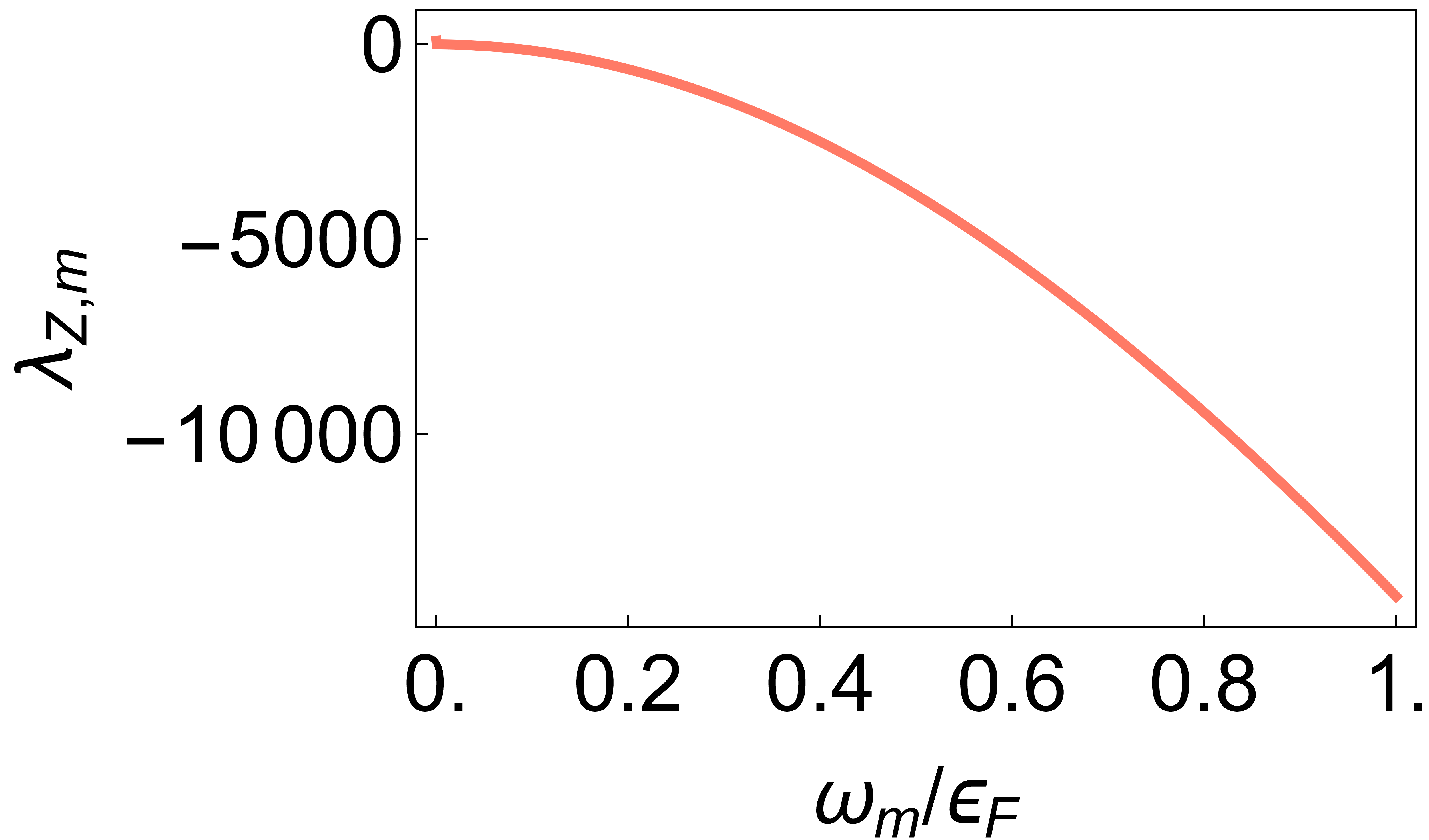
Now we are able to perform the integrals in Eqs. (56, 57). The frequency spectra are in Fig. H.2 below.

Refer to caption
Refer to caption
Figure H.2: The quasiparticle residue λZ,m\lambda_{Z,m} and the anomalous self-energy λϕ,m(l)\lambda_{\phi,m}^{(l)} for kF​d=1k_{F}d=1 and cutoff qc=10−5q_{c}=10^{-5}.

The behaviour of the anomalous self-energy λϕ,0(l)\lambda_{\phi,0}^{(l)} as a function of the layer separation is in absolute values for the l=0l=0 channel and in relative values for l=1,2l=1,2 in Fig. H.3. We see that the pairing strength decreases with increasing layer separation and that the ordering of the different channels remains unchanged.

Refer to caption
Refer to caption
Figure H.3: The anomalous self-energy λϕ,0(0)\lambda_{\phi,0}^{(0)} and the relative anomalous self-energy λϕ,0(0)−λϕ,0(l)\lambda_{\phi,0}^{(0)}-\lambda_{\phi,0}^{(l)} with cutoff qc=10−5q_{c}=10^{-5}.

Appendix I Density Imbalance

As can be seen from the Lagrangian in Eq. (6), the effective magnetic fields in the two layers are (taking the charge into account)

Beff+\displaystyle B_{\text{eff}}^{+} =B−4​π​n+,\displaystyle=B-4\pi n_{+}, (64)
Beff−\displaystyle B_{\text{eff}}^{-} =−B+4​π​n−.\displaystyle=-B+4\pi n_{-}. (65)

Using the relation n++n−=B2​πn_{+}+n_{-}=\frac{B}{2\pi}, we notice that the CEs and CHs experience exactly the same effective magnetic field Barkeshli et al. 2015.

Introducing a charge imbalance νT=(1/2−δ)+(1/2+δ)\nu_{T}=(1/2-\delta)+(1/2+\delta) between the two layers, we obtain the coupled Lagrangian near the mean-field solution

ℒCEL-CHL=∑s=+/−[ψ†s(∂τ+ia~τs+isdAτ−μs)ψs+12​msψ†s(i∇+𝒂~s+sd𝑨)2ψs+V(a~s)+s​i4​πa~τs∇∧𝒂~s]+V+⁣−​(a~+,a~−),\displaystyle\begin{split}\mathcal{L}_{\text{CEL-CHL}}=&\sum_{s=+/-}\bigg[\psi^{\dagger}_{s}\left(\partial_{\tau}+i\tilde{a}_{\tau}^{s}+isdA_{\tau}-\mu_{s}\right)\psi_{s}+\frac{1}{2m_{s}}\psi^{\dagger}_{s}\left(i\boldsymbol{\nabla}+\boldsymbol{\tilde{a}}^{s}+sd\boldsymbol{A}\right)^{2}\psi_{s}+V(\tilde{a}^{s})+\frac{si}{4\pi}\tilde{a}_{\tau}^{s}\boldsymbol{\nabla}\wedge\boldsymbol{\tilde{a}}^{s}\bigg]\\ &+V_{+-}(\tilde{a}^{+},\tilde{a}^{-}),\end{split} (66)

where d​AτdA_{\tau} denotes the remnant external field that is not cancelled by the flux attachment. This remnant field makes BeffB_{\text{eff}} in the two layers non-zero and pointing in opposite directions. This is true regardless of whether we describe the layers in terms of CEs or CHs. The additional effect from the density imbalance in the CEL-CHL Lagrangian appears from the last term above. However, since it is linear in the gauge fluctuations, it does not effect the theory and we can omit it from the Lagrangian. Thus, so far the charge imbalance has the same effect in the CEL-CEL as in the CEL-CHL. However, in the CEL-CHL theory, we should use CEs for the ν=1/2−δ\nu=1/2-\delta layer and CHs for the ν=1/2+δ\nu=1/2+\delta layer Barkeshli et al. 2015. This means that the Fermi surface shrinks in each of the two layers by the same amount. This is not the case in the CEL-CEL where the Fermi surface shrinks in one layer and expands in the other.