Optical IRSs: Power Scaling Law, Optimal Deployment, and Comparison with Relays This paper was presented in part at IEEE Globecom 2022 [1].

Hedieh Ajam¹ Marzieh Najafi¹ Vahid Jamali² Robert Schober¹ Affiliation: ¹Friedrich-Alexander-Universiät Erlangen-Nürnberg, ²Technical University of Darmstadt

Abstract

The line-of-sight (LOS) requirement of free-space optical (FSO) systems can be relaxed by employing optical relays or optical intelligent reflecting surfaces (IRSs). In this paper, we show that the power reflected from FSO IRSs and collected at the receiver (Rx) lens may scale quadratically or linearly with the IRS size or may saturate at a constant value. We analyze the power scaling law for optical IRSs and unveil its dependence on the wavelength, transmitter (Tx)-to-IRS and IRS-to-Rx distances, beam waist, and Rx lens size. We also consider the impact of linear, quadratic, and focusing phase shift profiles across the IRS on the power collected at the Rx lens for different IRS sizes. Our results reveal that surprisingly the powers received for the different phase shift profiles are identical, unless the IRS operates in the saturation regime. Moreover, IRSs employing the focusing (linear) phase shift profile require the largest (smallest) size to reach the saturation regime. We also compare optical IRSs in different power scaling regimes with optical relays in terms of the outage probability, diversity and coding gains, and optimal placement. Our results show that, at the expense of a higher hardware complexity, relay-assisted FSO links yield a better outage performance at high signal-to-noise-ratios (SNRs), but optical IRSs can achieve a higher performance at low SNRs. Moreover, while it is optimal to place relays equidistant from Tx and Rx, the optimal location of optical IRSs depends on the phase shift profile and the power scaling regime they operate in.

I Introduction

Due to their directional narrow laser beams and easy-to-install transceivers, free space optical (FSO) systems are promising candidates for high data rate applications, such as wireless front- and backhauling, in next generation wireless communication networks and beyond [2]. FSO systems require a line-of-sight (LOS) connection between transmitter (Tx) and receiver (Rx) which can be relaxed by using optical relays [3] or optical intelligent reflecting surfaces (IRSs) [4, 5]. Optical relays can either process and decode the received signal or only amplify it before retransmitting it to the Rx. For high data rate FSO systems, relays may require high-speed decoding and encoding hardware and/or analog gain units, additional synchronization, and clock recovery [6]. On the other hand, optical IRSs are planar structures comprised of passive subwavelength elements, known as unit cells, which can manipulate the properties of an incident wave such as its phase and polarization [7, 8]. In particular, to redirect an incident beam in a desired direction, the IRS can apply a phase shift to the incident wave and thereby adjust the accumulated phase of the reflected wave [9, 10]. Optical IRSs can be implemented using mirror- or metamaterial (MM)-based technologies [11] and, due to their passivity, incur a lower system complexity and power consumption than optical relays.

For radio frequency (RF) IRSs, by increasing the IRS area, $\Sigma_{\text{irs}}$ , the received power scales quadratically [12, 13]. For very large IRS sizes, the received power saturates at $\frac{1}{9}$ of the transmit power because as the IRS gets larger, its relative effective area (area perpendicular to the propagation direction) gets smaller [13]. However, there is a fundamental difference between FSO systems and the RF systems considered in [13]. In [13], the Rx area is smaller than a wavelength whereas optical lenses are typically much larger than a wavelength. Moreover, spherical/planar RF waves lead to a uniform power distribution across the IRS, whereas FSO systems employ Gaussian laser beams, which have a curved wavefront and a non-uniform power distribution [10]. Furthermore, the electrical size of the IRS (IRS length divided by the wavelength) at optical frequencies is much larger than at RF. Thus, we expect the power scaling law for optical IRSs to differ from that of RF IRSs. However, except for the preliminary results reported in the conference version of this paper [1], the power scaling law of optical IRSs has not been investigated yet.

In this paper, we analyze the power scaling law for optical IRSs in detail and show that depending on the Rx lens size, the locations of Tx and Rx with respect to (w.r.t.) the IRS, and the beam waist, the received power may scale quadratically ( $\mathcal{O}(\Sigma_{\text{irs}}^{2})$ ) or linearly ( $\mathcal{O}(\Sigma_{\text{irs}})$ ) with the IRS size or it may saturate to a constant value ( $\mathcal{O}(1)$ ). We will show that when both IRS and lens are smaller than footprint of the incident beam, the received power scales quadratically with the IRS size ( $\mathcal{O}(\Sigma_{\text{irs}}^{2})$ ). On the other hand, when the lens is larger than the beam footprint but the IRS is still smaller than the beam footprint, the received power scales linearly with the IRS size ( $\mathcal{O}(\Sigma_{\text{irs}})$ ). Finally, if both IRS and lens are larger than the footprint of the incident beam, the received power saturates at a constant value ( $\mathcal{O}(1)$ ).

Furthermore, we investigate the impact of different phase shift profiles of MM-based IRSs on the power scaling law. We show that for linear (LP), quadratic (QP), and focusing (FP) phase shift profiles the received powers at the lens are identical when the IRS operates in the quadratic and linear power scaling regimes. However, the adopted phase shift profile does affect the received power when the IRS operates in the saturation regime. In this case, the FP profile yields the largest received power as it focuses the total incident beam on the lens center, whereas the LP and QP profiles yield smaller values. In addition, we show that mirror-based IRSs outperform MM-based IRSs with LP profile due to their ability to adjust their orientation to the incident beam.

We also compare the performance of relay- and IRS-assisted FSO systems. Such comparisons were made between RF IRSs and decode-and-forward (DF) and amplify-and-forward (AF) relays in [14] and [15], respectively. However, RF links are fundamentally different from FSO links, where the variance of the fading is distance-dependent [3]. Moreover, to reduce hardware complexity, often half-duplex relays are preferred for RF systems, whereas FSO relays are typically full-duplex [16].

In this paper, we study relay- and IRS-assisted FSO systems where our contributions can be summarized as follows:

•

We analyze the power scaling law for different IRS and Rx lens sizes, and show that depending on the size of the beam footprint on the IRS and the lens, the received power may scale linearly or quadratically with the IRS size or it may remain constant.
•

We consider different phase shift profiles for MM-based IRSs and show that the impact of the phase profile is negligible when the IRS size is much smaller than the incident beam footprint on the IRS. However, when the IRS size is comparable to the beam footprint on the IRS, IRSs with QP and FP profiles perform better than IRSs with LP profile.
•

We compare the performance of IRS- and relay-assisted FSO systems in terms of their outage probability and their diversity and coding gains. Our results show that, at the expense of a higher hardware complexity, relay-assisted FSO links yield a higher diversity gain as the variance of the corresponding distance-dependent fading is smaller compared to that for IRS-assisted FSO links. Moreover, the coding gain in IRS-assisted FSO links may increase with the IRS size depending on the power scaling regime the IRS operates in.
•

We also analyze the optimal positions of FSO relays and IRSs for minimization of the end-to-end outage performance at high SNRs. We show that while relays are optimally positioned equidistant from Tx and Rx [17, 16], the optimal position of optical IRSs depends on the power scaling regime they operate in as well as the IRS technology and phase shift profile. In particular, at the expense of a large form factor needed for rotation, mirror-based IRSs perform identical at any position between Tx and Rx. In contrast, MM-based IRSs with LP profile achieve optimal outage performance close to Tx, close to Tx or Rx, and equidistant from Tx and Rx when they operate in the linear, quadratic, and saturation power scaling regime, respectively. Furthermore, for IRSs operating in the saturation regime, employing the QP or FP profiles can be advantageous. For the QP profile, by changing the focal parameter, the optimal position of the IRS can be adjusted. For the FP profile, the IRS can achieve the optimal outage performance for a large range of Tx-to-IRS distances rather than at a single point.

To the best of the authors’ knowledge, a power scaling law for optical IRSs with LP profile and a performance comparison with relays were first reported in [1], which is the conference version of this paper. In contrast to [1], in this paper, we do not only consider IRSs with LP profile but also with QP and FP profiles and investigate the impact of the phase shift profile on the power scaling law. Moreover, the optimal positions of IRSs with QP and FP profiles were not studied in [1].

Notations: Boldface lower-case and upper-case letters denote vectors and matrices, respectively. Superscript $(\cdot)^{T}$ and $\mathbb{E}\{\cdot\}$ denote the transpose and expectation operators, respectively. $x\sim\mathcal{N}(\mu,\sigma^{2})$ represents a Gaussian random variable with mean $\mu$ and variance $\sigma^{2}$ . $\mathbf{I}_{n}$ is the $n\times n$ identity matrix, $j$ denotes the imaginary unit, and $(\cdot)^{*}$ and $\mathcal{R}\{\cdot\}$ represent the complex conjugate and real part of a complex number, respectively. Moreover, $\text{erf}(\cdot)$ and $\text{erfi}(\cdot)$ are the error function and the imaginary error function, respectively. Here, $\Phi(x)=\int_{-\infty}^{x}\frac{1}{\sqrt{2\pi}}e^{-\frac{t^{2}}{2}}\mathrm{d}t$ denotes the cumulative distribution function (CDF) of the univariate normal density. Furthermore, $\mathbb{R}^{+}$ denotes the set of positive real numbers. $\lVert\cdot\rVert$ denotes the vector $\ell_{2}$ -norm and $\text{sinc}(x)=\frac{\sin(x)}{x}$ is the sinc function.

II System and Channel Models

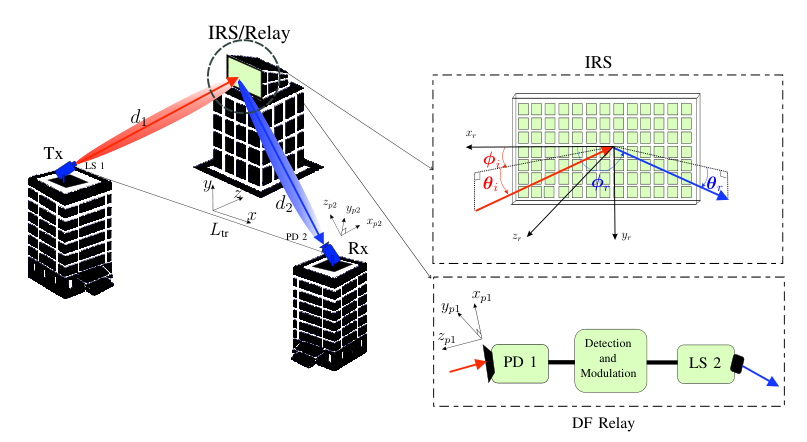
Refer to caption — Fig. 1: IRS- and relay-based FSO systems.

We consider two FSO systems, where Tx and Rx are connected via an IRS and a relay, respectively. Tx and Rx are located on the $x$ -axis with distance $L_{\text{tr}}\over 2$ from the origin of the $xyz$ -coordinate system, respectively, see Fig. 1. Moreover, the centers of the IRS and the relay are located at the origin of the $x_{r}y_{r}z_{r}$ -coordinate system, where the $x_{r}y_{r}$ -plane is parallel to the $xy$ -plane and the $z_{r}$ -axis points in the opposite direction of the $z$ -axis, see Fig. 1. The Tx is equipped with laser source (LS) 1 emitting a Gaussian laser beam. The beam axis intersects with the $x_{r}y_{r}$ -plane at distance $d_{1}$ and points in direction $\mathbf{\Psi}_{i}=\left(\theta_{i},\phi_{i}\right)$ , where $\theta_{i}$ is the angle between the $x_{r}y_{r}$ -plane and the beam axis, and $\phi_{i}$ is the angle between the projection of the beam axis on the $x_{r}y_{r}$ -plane and the $x_{r}$ -axis. Moreover, the Rx is equipped with photo-detector (PD) 2 and a circular lens of radius $a$ . The lens of the Rx is located at distance $d_{2}$ from the origin of the $x_{r}y_{r}z_{r}$ -coordinate system. The normal vector of the lens plane points in direction $\mathbf{\Psi}_{r}=\left(\theta_{r},\phi_{r}\right)$ , where $\theta_{r}$ is the angle between the $x_{r}y_{r}$ -plane and the normal vector, and $\phi_{r}$ is the angle between the projection of the normal vector on the $x_{r}y_{r}$ -plane and the $x_{r}$ -axis. Furthermore, we assume that Tx, Rx, IRS, and relay are installed at the same height, i.e., $\phi_{i}=0$ and $\phi_{r}=\pi$ , and the Rx lens plane is always perpendicular to the axis of the received beam. In the following, we describe the relay- and IRS-assisted FSO systems more in detail.

II-A Relay-Assisted FSO System Model

We assume the Tx is connected to the Rx via a full-duplex DF relay¹¹ 1 In this work, we assume DF relaying, as under typical channel conditions, it achieves better or at least similar performance compared to AF relaying [16]., where the relay receives the transmitted symbols via PD 1, re-encodes the signal, and transmit it via LS 2 to PD 2 at the Rx. PD 1 is equipped with a circular lens of radius $a$ , which is always perpendicular to the axis of the received beam. Assuming an intensity modulation and direct detection (IM/DD) system, the received signal at the relay, $y_{1}$ , is given by

\displaystyle y_{1}

\displaystyle=\sqrt{P_{1}}h_{1}s_{1}+n_{1},

(1)

where $s_{1}$ is the symbol transmitted by LS 1 with $\mathbb{E}\{|s_{1}|^{2}\}=1$ , $P_{1}$ is the transmit power of LS 1, $h_{1}\in\mathbb{R}^{+}$ denotes the gain of the Tx-relay link, and $n_{1}\sim\mathcal{N}\left(0,\sigma_{n}^{2}\right)$ is the additive white Gaussian noise (AWGN) at PD 1 with zero mean and variance $\sigma_{n}^{2}$ . Then, the received signal at PD 2, $y_{2}$ , is given by

\displaystyle y_{2}

\displaystyle=\sqrt{P_{2}}h_{2}s_{2}+n_{2},

(2)

where $s_{2}$ is the signal transmitted by the relay with $\mathbb{E}\{|s_{2}|^{2}\}=1$ , $h_{2}\in\mathcal{R}^{+}$ denotes the FSO channel gain of the relay-Rx link, $P_{2}$ is the transmit power of LS 2, and $n_{2}\sim\mathcal{N}\left(0,\sigma_{n}^{2}\right)$ is the AWGN noise at PD 2. For simplicity, $P_{1}$ and $P_{2}$ are chosen such that $P_{1}=P_{2}=\frac{P_{\text{tot}}}{2}$ , where $P_{\text{tot}}$ is the total transmit power.

II-B IRS-Assisted FSO System Model

We assume the Tx is connected via a single IRS to the Rx. The size of the IRS is $\Sigma_{\text{irs}}=L_{x}\times L_{y}$ , where $L_{x}$ and $L_{y}$ are the lengths of the IRS in $x_{r}$ - and $y_{r}$ -direction, respectively. Optical IRSs can be implemented using mirror-based or MM-based technologies [11]. Here, we consider the following setups:

•

Mirror-based IRSs: A single conventional mirror or an array of small micro-mirrors can be employed to provide specular reflection, i.e., the incident and reflected beam angles w.r.t. the IRS are identical. To provide the desired reflection angle, the mirror can be re-oriented with a mechanical motor, which rotates the mirror with elevation and azimuth angles $\Theta_{\text{mir}}=\frac{|\theta_{r}-\theta_{i}|}{2}$ and $\varphi_{\text{mir}}=\frac{|\pi-\phi_{r}+\phi_{i}|}{2}$ , respectively. Since $\phi_{i}=0$ and $\phi_{r}=\pi$ , the azimuth angle is given by $\varphi_{\text{mir}}=0$ .

•

MM-based IRSs: An MM-based IRS is a planar surface which is comprised of passive sub-wavelength elements to manipulate the properties of the incident beam. Since typically $L_{x},L_{y}\gg\lambda$ , where $\lambda$ is the wavelength, MM-based IRSs can be modeled as continuous surfaces with continuous phase shift profile. The following phase shift designs are considered in this paper:

1.

Linear phase shift (LP) profile: Anomalous reflection and redirection of the beam originating from the LS towards the lens is accomplished with an IRS phase shift profile which changes linearly along the $x_{r}$ - and $y_{r}$ -axes as follows [18]:

$\displaystyle\Phi_{\text{irs}}({\mathbf{r}_{r}})=k\left(\Phi_{x}x_{r}+\Phi_{y}y_{r}+\Phi_{0}\right),$ (3)

where $k=\frac{2\pi}{\lambda}$ is the wave number and $\mathbf{r}_{r}=(x_{r},y_{r},0)$ denotes a point in the $x_{r}y_{r}$ -plane. To redirect the beam from Tx direction $\mathbf{\Psi}_{i}$ to Rx direction $\mathbf{\Psi}_{r}$ , the phase shift gradients are chosen as $\Phi_{x}=\cos(\theta_{i})\cos(\phi_{i})+\cos(\theta_{r})\cos(\phi_{r})$ , $\Phi_{y}=\cos(\theta_{i})\sin(\phi_{i})+\cos(\theta_{r})\sin(\phi_{r})$ , and $\Phi_{0}$ is constant.

Quadratic phase shift (QP) profile: Focusing the beam at distance $f$ from the IRS along direction $\mathbf{\Psi}_{r}$ and reducing the beamwidth of the reflected beam can be realized with a phase shift profile which changes quadratically along the $x_{r}$ - and $y_{r}$ -axes, respectively. Thus, we consider the following phase shift profile which eliminates the accumulated phase of the incident beam and adds a parabolic phase shift [10]:

\displaystyle\Phi_{\text{irs}}(\mathbf{r}_{r})=k\left(\Phi_{x^{2}}x_{r}^{2}+\Phi_{y^{2}}y_{r}^{2}+\Phi_{x}x_{r}+\Phi_{y}y_{r}+\Phi_{0}\right),

(4)

where $\Phi_{x^{2}}=-\frac{\sin^{2}(\theta_{i})}{2R(d_{1})}-\frac{\sin^{2}(\theta_{r})}{2d_{2}}+\frac{\sin^{2}(\theta_{r})}{4f}$ and $\Phi_{y^{2}}=-\frac{1}{2R(d_{1})}-\frac{1}{2d_{2}}+\frac{1}{4f}$ .

3.

Focusing phase shift (FP) profile: An ideal phase shift profile, which focuses the incident beam power on the lens center, is given as follows

$\displaystyle\Phi_{\text{irs}}(\mathbf{r}_{r})=-\psi_{\text{in}}-k\lVert\tilde{\mathbf{r}}_{o}-\mathbf{r}_{r}\rVert,$ (5)

where $\tilde{\mathbf{r}}_{o}=(\tilde{x}_{o},\tilde{y}_{o},\tilde{z}_{o})=(-d_{2}\cos\theta_{p},0,d_{2}\sin\theta_{p})$ denotes the center of the lens and $\psi_{\text{in}}$ is the phase of the incident beam on the IRS.

The above considered technologies and phase shift profiles enhance the end-to-end FSO link performance as follows: An MM-based IRS with LP profile behaves similarly to a mirror in redirecting the beam towards the Rx but the latter can direct more power towards the Rx lens because of the larger effective IRS aperture achieved by its reorientation facilitated by mechanical motors. Moreover, an IRS with QP profile can reduce the beamwidth at the lens and mitigate beam divergence along the propagation path. Furthermore, an IRS with FP profile yields a very narrow beam at the lens such that the lens can collect most of the transmitted power in the absence of misalignment and tracking errors.

Assuming an IM/DD FSO system, regardless of the adopted phase shift profile, for an IRS-assisted FSO link the received signal $y_{3}$ at PD 2, is given by

\displaystyle y_{3}=\sqrt{P_{\text{tot}}}h_{3}s_{1}+n_{2},

(6)

where $h_{3}\in\mathcal{R}^{+}$ is the end-to-end channel gain between Tx, IRS, and Rx and LS 1 transmits with power $P_{\text{tot}}$ .

II-C Channel Model

FSO channels are impaired by geometric and misalignment losses (GML), atmospheric loss, and atmospheric turbulence induced fading [18]. Thus, the point-to-point FSO channel gains of the considered systems can be modeled as follows

\displaystyle h_{i}=\zeta h_{p,i}h_{a,i}h_{\text{gml},i},\quad i\in\{1,2,3\},

(7)

where $\zeta$ is the PD responsivity, $h_{a,i}$ represents the random atmospheric turbulence induced fading, $h_{p,i}$ is the atmospheric loss, and $h_{\text{gml},i}$ characterizes the GML.

II-C1 Atmospheric Loss

The atmospheric loss characterizes the laser beam energy loss due to absorption and scattering and is given by $h_{p,i}=10^{-\frac{\kappa d_{i}}{10}},i\in\{1,2,3\},$ where $\kappa$ is the attenuation coefficient and $d_{3}=d_{1}+d_{2}$ denotes the end-to-end link distance.

II-C2 Atmospheric Turbulence

The variations of the refractive index along the propagation path due to changes in temperature and pressure cause atmospheric turbulence which is analogous to the fading in RF systems. Assuming $h_{a,i}$ is a Gamma-Gamma distributed random variable, its cumulative distribution function (CDF) is given by [19]

\displaystyle F_{h_{a,i}}(x)=\frac{1}{\Gamma(\alpha_{i})\Gamma(\beta_{i})}G_{1,3}^{2,1}\left(\alpha_{i}\beta_{i}{{x}}\left|\begin{array}[]{@{}l@{}}\ \ \ \ \ \ \ 1\\ \alpha_{i},\beta_{i},0\\ \end{array}\right.\right),

where $\Gamma(\cdot)$ denotes the Gamma function and $G_{p,q}^{m,n}\left(\varkappa\left|\begin{array}[]{@{}l@{}}e_{1},\dots e_{p}\\ f_{1},\dots,f_{q}\\ \end{array}\right.\right)$ is the Meijer G-function [20]. Here, the small and large scale turbulence parameters $\alpha_{i}$ and $\beta_{i}$ depend on the Rytov variance $\sigma_{R,i}^{2}=1.23C_{n}^{2}k^{7\over 6}d_{i}^{11\over 6}$ , where $C_{n}^{2}$ is the refractive-index structure constant [16]. Given that $d_{3}>d_{1},d_{2}$ , the Ryotov variance of the IRS-assisted link is larger, which leads to more severe fading compared to the relay-assisted link.

II-C3 GML

The GML coefficient comprises the deterministic geometric loss due to the divergence of the laser beam along the transmission path and the random misalignment loss due to transceiver sway [11]. Here, we neglect the misalignment loss ²² 2 In practice, the misalignment loss can be avoided or considerably reduced by using sophisticated acquisition and tracking mechanisms such as gimbals, mirrors, and adaptive optics [21]. and determine the geometric loss for the relay- and IRS-based links in the following.

Assuming the waist of the Gaussian beam is larger than the wavelength, the electric field of the Gaussian laser beam emitted by the $i$ -th LS, $\forall i\in\{1,2\}$ , is given by [22]

\displaystyle E_{\ell i}\!\left(\mathbf{r}_{\ell i}\right)

\displaystyle=C_{\ell}e^{-{x_{\ell i}^{2}+y_{\ell i}^{2}\over w^{2}(z_{\ell i})}-jk\left(\!\!z_{\ell i}+{x_{\ell i}^{2}+y_{\ell i}^{2}\over 2R(z_{\ell i})}\right)-\tan^{-1}\left(\frac{z_{\ell i}}{z_{Ri}}\right)},\qquad

(11)

where $C_{\ell}=\sqrt{\frac{4\eta P_{\text{tot}}}{n\pi{w}^{2}(z_{\ell i})}}$ , $\eta$ is the free-space impedance, $n=1$ and $2$ for the IRS- and relay-assisted links, respectively, and $\mathbf{r}_{\ell i}=(x_{\ell i},y_{\ell i},z_{\ell i})$ is a point in a coordinate system, which has its origin at the $i$ -th LS. The $z_{\ell i}$ -axis of this coordinate system is along the beam axis, the $y_{\ell i}$ -axis is parallel to the intersection line of the $i$ -th LS plane and the $x_{r}y_{r}$ -plane, and the $x_{\ell i}$ -axis is orthogonal to the $y_{\ell i}$ - and $z_{\ell i}$ -axes. $w(z_{\ell i})=w_{oi}\Big[{1+\left(\frac{z_{\ell i}}{z_{Ri}}\right)^{2}}\Big]^{1/2}$ is the beamwidth at distance $z_{\ell i}$ , $w_{oi}$ is the beam waist, $z_{Ri}=\frac{\pi w_{oi}^{2}}{\lambda}$ is the Rayleigh range, and $R(z_{\ell i})=z_{\ell i}\Big[1+\left(\frac{z_{Ri}}{z_{\ell i}}\right)^{2}\Big]$ is the radius of the curvature of the beam’s wavefront.

Assuming the lenses at the relay and the Rx are always perpendicular to the incident beam axes, respectively, the GML coefficients of the Tx-relay link, $h_{\text{gml},1}$ , and the relay-Rx link, $h_{\text{gml},2}$ , are given by [23]

\displaystyle h_{\text{gml},i}={1\over\eta P_{\text{tot}}}\iint\nolimits_{\mathcal{A}_{pi}}\lvert E_{\ell i}\left(\mathbf{r}_{pi}\right)\rvert^{2}\,\mathrm{d}\mathcal{A}_{pi},\,\quad i\in\{1,2\},

(12)

where $\mathcal{A}_{pi}$ denotes the area of the lens of PD $i$ and $\mathbf{r}_{pi}=(x_{pi},y_{pi},z_{pi})$ denotes a point in the $i$ -th lens plane. The origin of the $x_{pi}y_{pi}z_{pi}$ -coordinate system is the center of the $i$ -th lens and the $z_{pi}$ -axis is parallel to the normal vector of the $i$ -th lens plane. We assume that the $y_{pi}$ -axis is parallel to the intersection line of the lens plane and the $x_{r}y_{r}$ -plane and the $x_{pi}$ -axis is perpendicular to the $y_{pi}$ - and $z_{pi}$ -axes. Moreover, the GML coefficient of the IRS-assisted FSO link is given by [10]

\displaystyle h_{\text{gml},3}={1\over 2\eta P_{\text{tot}}}\iint\nolimits_{\mathcal{A}_{p2}}\lvert E_{r}\left(\mathbf{r}_{p2}\right)\rvert^{2}\,\mathrm{d}\mathcal{A}_{p2},\quad

(13)

where $E_{r}\left(\mathbf{r}_{p2}\right)$ is the electric field of the beam reflected by the IRS and received at the Rx lens and is given by [10]

\displaystyle E_{r}\left(\mathbf{r}_{p2}\right)=C_{r}\iint_{({x}_{r},{y}_{r})\in\Sigma_{\text{irs}}}E_{\text{in}}({\mathbf{r}_{r}})\exp\left(-jk\lVert\mathbf{r}_{o}-\mathbf{r}_{r}\rVert\right)e^{-j\Phi_{\text{irs}}(\mathbf{r}_{r})}\mathrm{d}{x}_{r}\mathrm{d}{y}_{r}.\quad

(14)

Here, $C_{r}={\sqrt{\sin(\theta_{r})}}/({j\lambda d_{2}})$ , $\mathbf{r}_{o}=\left(\mathbf{r}_{p2}+\mathbf{c}_{1}\right)\mathbf{R}_{\text{rot}}$ , $\mathbf{R}_{\text{rot}}=\left(\begin{smallmatrix}-\sin(\theta_{r})&0&-\cos(\theta_{r})\\ 0&-1&0\\ -\cos(\theta_{r})&0&\sin(\theta_{r})\end{smallmatrix}\right)$ , $\mathbf{c}_{1}=(0,0,d_{2})$ , and $E_{\text{in}}({\mathbf{r}_{r}})$ is the electric field incident on the IRS given in [10, Eq. (7)] as follows

	$\displaystyle E_{\text{in}}(\mathbf{r}_{r})$	$\displaystyle=C_{\ell}\sqrt{\|\sin(\theta_{i})\|}e^{-\frac{x_{r}^{2}}{w^{2}_{\text{in},x}}-\frac{y_{r}^{2}}{w^{2}_{\text{in},y}}-j\psi_{\text{in}}(\mathbf{r}_{r})}\quad\text{with phase}$
	$\displaystyle\psi_{\text{in}}(\mathbf{r}_{r})$	$\displaystyle=k\left(d_{1}-x_{r}\cos(\theta_{i})+\frac{x_{r}^{2}\sin^{2}(\theta_{i})}{2R(d_{1})}+\frac{y_{r}^{2}}{2R(d_{1})}\right)-\tan^{-1}\left(\frac{d_{1}}{z_{R1}}\right),$			(15)

where $w_{\text{in},x}=\frac{w(d_{1})}{\sin(\theta_{i})}$ and $w_{\text{in},y}=w(d_{1})$ are the incident beamwidths in the IRS plane in $x$ - and $y$ -direction, respectively. A closed-form solution of (13) for IRSs with LP and QP profiles operating at intermediate- and far-field distances (Fresnel regime), i.e., $d_{2}\gg d_{n}$ , where $d_{n}=\left[\frac{(x_{e}^{2}+y_{e}^{2})(x_{e}+y_{e})}{4\lambda}\right]^{\frac{1}{2}}$ and $i_{e}=\min(\frac{L_{i}}{2},w_{\text{in},i})$ , $i\in\{x,y\}$ , is given by [10, Eq. (20)]³³ 3 For a typical FSO link with $w_{o1}=2.5$ mm, $d_{1}=d_{2}=700$ m, $\theta_{i}=\theta_{r}=\frac{\pi}{4}$ and square-shaped IRS with length $0.5$ m, we have $x_{e}=0.2$ m, $y_{e}=0.14$ m, which leads to $d_{n}=55$ m. This means that for distances $d_{2}>55\,\text{m}$ , the result in [10, Eq. (20)] is valid. Unfortunately, [10, Eq. (20)] is a very involved expression and cannot be used to derive the dependence of the received power on the IRS and lens sizes and also does not provide insight into the end-to-end system performance. Thus, in the following, we reanalyze (13) for different IRS and lens sizes to derive power scaling law for optical IRS.

III Power Scaling Law for Optical IRSs

In this section, we analyze the received power at the Rx lens for mirror-based and MM-based IRSs with different phase shift profiles. The received power at the lens for the IRS-assisted link using (6) and (7) is given by

\displaystyle P_{\text{rx}}^{\text{irs}}=P_{\text{tot}}\zeta^{2}h_{p,3}^{2}h_{a,3}^{2}h_{\text{gml},3}^{2},

(16)

where only the GML factor $h_{\text{gml},3}$ depends on the IRS and lens sizes. In this paper, to gain insight for FSO system design and to determine the corresponding power scaling law, we analyze $h_{\text{gml},3}$ given by (13) and (14) for different IRS sizes, $\Sigma_{\text{irs}}$ , and lens sizes, $\Sigma_{\text{lens}}$ , as follows:

•

Regime 1: $\Sigma_{\text{irs}}\ll A_{\text{in}}$ and $\Sigma_{\text{lens}}\ll A_{\text{rx}}^{\text{g1}}$
•

Regime 2: $\Sigma_{\text{irs}}\ll A_{\text{in}}$ and $\Sigma_{\text{lens}}\gg A_{\text{rx}}^{\text{g2}}$
•

Regime 3: $\Sigma_{\text{irs}}\gg A_{\text{in}}$

where $A_{\text{in}}=\pi w_{\text{in},x}w_{\text{in},y}$ and $A_{\text{rx}}^{q}=\pi w_{\text{rx},x}^{\iota,q}w_{\text{rx},y}^{\iota,q}$ are the areas of the equivalent beam footprints in the IRS and Rx lens planes, respectively. Moreover, $w_{\text{rx},x}^{\iota,q}$ and $w_{\text{rx},y}^{\iota,q}$ are the equivalent received beam widths in the lens plane in $x_{p}$ - and $y_{p}$ -direction, respectively. Here, ${q}\in\{\text{g1},\text{g2},\text{g3}\}$ denotes the operating regime of the IRS and $\iota\in\{\text{LP},\text{QP},\text{FP},\text{mir}\}$ indicates the IRS technology and phase shift profile. In the following, we show that depending on the system parameters, the GML, and hence, the received power scales quadratically or linearly with the IRS size or it may remain constant.

III-A Regime 1: Quadratic Power Scaling Regime

In this regime, we consider the case where the IRS is small such that only a fraction of the Gaussian incident beam is captured by the IRS and the beam can be approximated by a plane wave. We derive the GML coefficient using the plane wave approximation in Lemma 1. Then, for a lens smaller than the received beam footprint, the GML coefficient is approximated in Corollary 1.

Lemma 1

Assuming an Rx lens at distances $d_{2}\gg d_{n}$ and an IRS with

•

LP profile and $L_{x}\ll\min\{w_{\text{in},x},\sqrt{\frac{2d_{1}d_{2}}{kd_{3}}}\}$ , $L_{y}\ll\min\{w_{\text{in},y},\sqrt{\frac{2d_{1}d_{2}}{kd_{3}}}\}$
•

QP profile and $L_{x}\ll\min\{w_{\text{in},x},\sqrt{\frac{4f}{k}}\}$ and $L_{y}\ll\min\{w_{\text{in},y},\sqrt{\frac{4f}{k}}\}$
•

FP profile and $L_{x}\ll w_{\text{in},x}$ and $L_{y}\ll w_{\text{in},y}$

the GML coefficient for the IRS-assisted link, $h_{\text{gml},3}$ , can be approximated by $\tilde{G}_{1}^{\iota}$ , which is given as follows

	$\displaystyle\tilde{G}_{1}^{\iota}=C_{1}$	$\displaystyle\left[\frac{a\sqrt{\pi}}{w_{\text{rx},x}^{\iota,\text{g1}}}\text{Si}\left(\frac{a\sqrt{\pi}}{w_{\text{rx},x}^{\iota,\text{g1}}}\right)+\cos\left(\frac{a\sqrt{\pi}}{w_{\text{rx},x}^{\iota,\text{g1}}}\right)-1\right]$
	$\displaystyle\times$	$\displaystyle\left[\frac{a\sqrt{\pi}}{w_{\text{rx},y}^{\iota,\text{g1}}}\text{Si}\left(\frac{a\sqrt{\pi}}{w_{\text{rx},y}^{\iota,\text{g1}}}\right)+\cos\left(\frac{a\sqrt{\pi}}{w_{\text{rx},y}^{\iota,\text{g1}}}\right)-1\right],\quad\iota\in\{\text{LP},\text{QP},\text{FP}\},$			(17)

where $C_{1}=\frac{8d_{2}^{2}\lambda^{2}\left|\sin(\theta_{i})\right|}{\pi^{6}a^{2}w^{2}(d_{1})\left|\sin(\theta_{r})\right|}$ , $\text{Si}(\varkappa)=\int_{0}^{\varkappa}\frac{\sin(t)}{t}\mathrm{d}t$ denotes the sine integral function, and $w_{\text{rx},x}^{\iota,\text{g1}}=\frac{2d_{2}}{k\sin(\theta_{r})L_{x}}$ , $w_{\text{rx},y}^{\iota,\text{g1}}=\frac{2d_{2}}{kL_{y}}$ can be interpreted as equivalent beamwidths.

Proof:

The proof is given in Appendix A. ∎Lemma 1 reveals that due to the small IRS size, the GML coefficient is independent of the considered IRS phase shift profile. Furthermore, due to the small IRS size, the amplitude of the received electric field is the product of two sinc-functions, see (42) in Appendix A. Thus, the coherent superposition of the signals reflected from all points on the IRS at the lens introduces a beamforming gain. By increasing the IRS size, the beamwidth of the sinc-shaped beam at the lens decreases, which in turn increases the peak amplitude of the beam causing the beamforming gain. In addition to this beamforming gain, a larger IRS surface collects more power from the incident beam which results in a quadratic scaling of the power received at the Rx lens with the IRS size. This behavior is analytically confirmed in the following corollary.

Corollary 1

For $\Sigma_{\text{lens}}\ll A_{\text{rx}}^{\text{g1}}$ and $d_{1}\gg z_{R1}$ , $\tilde{G}_{1}^{\iota}$ can be approximated by

\displaystyle{G}_{1}^{\iota}

\displaystyle=\frac{16\pi^{2}\Sigma_{\text{irs}}^{2}\left|\sin(\theta_{r})\right|\left|\sin(\theta_{i})\right|}{\lambda^{4}}\times g_{\text{LS}}\times g_{\text{PD}},\quad\iota\in\{\text{LP},\text{QP},\text{FP}\},

(18)

where $g_{\text{LS}}=\frac{2\pi w_{o1}^{2}}{4\pi d_{1}^{2}}$ and $g_{\text{PD}}=\frac{\pi a^{2}}{4\pi d_{2}^{2}}$ . Since $G_{1}^{\iota}$ scales quadratically with the IRS size, $\Sigma_{\text{irs}}$ , we refer to this regime as the “quadratic power scaling regime”.

Proof:

Assuming $a\sqrt{\pi}\ll\min\{w_{\text{rx},x}^{\iota,\text{g1}},w_{\text{rx},y}^{\iota,\text{g1}}\}$ , we substitute in (17) the Taylor series expansions of $\text{Si}(x)\approx x$ and $\cos(x)\approx 1-\frac{x^{2}}{2}$ . Then, assuming $d_{1}\gg z_{R1}$ , we can substitute $w(d_{1})\approx\frac{d_{1}\lambda}{\pi w_{o1}}$ . This completes the proof. ∎The quadratic scaling law shown in Corollary 1 is in agreement with the power scaling law in [24, Eq. (2), (10)] and [13, Eq. (48)] for RF IRSs.

Corollary 2

Assuming a mirror-based IRS of size $\Sigma_{\text{irs}}\ll\min\{A_{\text{in}},\frac{2d_{1}d_{2}}{kd_{3}}\}$ , which can mechanically rotate around the $z_{r}$ -axis with rotation angle $\Theta_{\text{mir}}=\frac{|\theta_{r}-\theta_{i}|}{2}$ , and an Rx lens size $\Sigma_{\text{lens}}\ll A_{\text{rx}}^{\text{g1}}$ , the GML for a mirror-assisted link, $h_{\text{gml},3}$ , can be approximated by ${G}_{1}^{\text{mir}}$ , which is given as follows

\displaystyle{G}_{1}^{\text{mir}}

\displaystyle=\frac{16\pi^{2}\Sigma_{\text{irs}}^{2}\left|\sin(\theta_{i}^{\text{mir}})\right|^{2}}{\lambda^{4}}\times g_{\text{LS}}\times g_{\text{PD}}.\quad

(19)

where $\theta_{i}^{\text{mir}}=\frac{\theta_{i}+\theta_{r}}{2}$ .

Proof:

Given the rotation angle of the mirror $\Theta_{\text{mir}}$ , we can substitute $\theta_{i}$ and $\theta_{r}$ in (14) with $\theta_{i}^{\text{mir}}$ and $\theta_{r}^{\text{mir}}$ , respectively, where $\theta_{i}^{\text{mir}}=\theta_{r}^{\text{mir}}$ due to the specular reflection. Then, for a mirror, $\Phi_{\text{irs}}=0$ and following similar steps as in Appendix A leads to (19). This completes the proof. ∎

III-B Regime 2: Linear Power Scaling Regime

As the size of the IRS increases, eventually the beamforming gain of the IRS saturates and cannot further increase the received power. In this regime, the lens is much larger than the beam footprint at the Rx such that the total power incident on the IRS is received at the Rx lens. Thus, by further increasing the IRS size, the received power increases only linearly. In the following lemma, we provide the GML for this case.

Lemma 2

Assuming $a\gg\min\{w_{\text{rx},x}^{\iota,\text{g2}},w_{\text{rx},y}^{\iota,\text{g2}}\}$ , where $w_{\text{rx},i}^{\iota,\text{g2}}=\frac{2\sqrt{\tilde{b}_{i,\iota}}}{k},\forall i\{x,y\}$ , are the equivalent beamwidths in the linear power regime, the GML factor for an IRS with phase shift profile $\iota$ , $h_{\text{gml},3}^{\iota}$ , can be approximated by $\tilde{G}_{2}^{\iota}$ , which is given as follows

\displaystyle\tilde{G}_{2}^{\iota}=

\displaystyle\frac{1}{16}\left[8\text{T}(a_{1},c_{2,1})+8\text{T}(a_{1}^{*},c_{2,1}^{*})+4\right]\left[8\text{T}(a_{2},c_{2,2})+8\text{T}(a_{2}^{*},c_{2,2}^{*})+4\right],\iota\in\{\text{LP},\text{QP},\text{FP}\},\quad

(20)

where $\text{T}(\cdot,\cdot)$ is the Owen’s T function [25], $a_{m}=\frac{\sqrt{2}\zeta_{1,m}}{\sqrt{1+2\zeta_{2,m}^{2}}}$ , $c_{2,m}=-\frac{\zeta_{1,m}^{*}\left(1+2\zeta_{2,m}^{2}+2\frac{\zeta_{1,m}}{\zeta_{1}^{*}}|\zeta_{2,m}|^{2}\right)}{\zeta_{1,m}\sqrt{1+2\zeta_{2,m}^{2}+2(\zeta_{2,m}^{*})^{2}}}$ , $m\in\{1,2\}$ , $\zeta_{1,1}=\frac{\sqrt{b_{x,\iota}}L_{x}}{2}$ , $\zeta_{2,1}=j\frac{\sqrt{b_{x,\iota}^{*}}}{2\sqrt{B_{x,\iota}}}$ , ${\zeta}_{1,2}=\frac{\sqrt{b_{y,\iota}}L_{y}}{2}$ , ${\zeta}_{2,2}=j\frac{\sqrt{b_{y,\iota}^{*}}}{2\sqrt{B_{y,\iota}}}$ , $b_{x,\text{LP}}=\frac{\sin^{2}(\theta_{i})}{w^{2}(d_{1})}+\frac{jk\sin^{2}(\theta_{i})}{2R(d_{1})}+\frac{jk\sin^{2}(\theta_{r})}{2d_{2}}$ , $b_{y,\text{LP}}=\frac{1}{w^{2}(d_{1})}+\frac{jk}{2R(d_{1})}+\frac{jk}{2d_{2}}$ , $b_{x,\text{QP}}=\frac{\sin^{2}(\theta_{i})}{w^{2}(d_{1})}+\frac{jk\sin^{2}(\theta_{r})}{4f}$ , $b_{y,\text{QP}}=\frac{1}{w^{2}(d_{1})}+\frac{jk}{4f}$ , $b_{x,\text{FP}}=\frac{\sin^{2}(\theta_{i})}{w^{2}(d_{1})}$ , $b_{y,\text{FP}}=\frac{1}{w^{2}(d_{1})}$ , $B_{i,\iota}=\mathcal{R}\{b_{i,\iota}\}$ , and $\tilde{b}_{i,\iota}=\frac{{b}_{i,\iota}{b}_{i,\iota}^{*}}{{b}_{i,\iota}+{b}_{i,\iota}^{*}}$ .

Proof:

The proof is provided in Appendix B. ∎In (20), by assuming large lens sizes, $\tilde{G}_{2}^{\iota}$ only depends on the IRS size and phase shift profile. To unveil the second power scaling regime, we approximate (20) in the following corollary.

Corollary 3

Assuming $\Sigma_{\text{irs}}\ll A_{\text{in}}$ , $\tilde{G}_{2}^{\iota}$ can be approximated by

\displaystyle\bar{G}_{2}^{\iota}

\displaystyle=\text{erf}\left(\frac{\sqrt{2}}{2}\frac{L_{x}\sin(\theta_{i})}{w(d_{1})}\right)\text{erf}\left(\frac{\sqrt{2}}{2}\frac{L_{y}}{w(d_{1})}\right).\quad

(21)

Proof:

We approximate $c_{2,i}\to-\infty$ and we exploit $\text{T}(x,\infty)=\frac{1-\Phi(|x|)}{2}$ in [25, pp. 414, Eq. (2.4)] to obtain $\tilde{G}_{2}^{\iota}=\frac{1}{16}\left[-4+8\Phi(|a_{1}|)\right]\left[-4+8\Phi(|a_{2}|)\right]$ . Substituting $\Phi(x)=\frac{1}{2}\text{erf}\left(\frac{x}{\sqrt{2}}+1\right)$ , we obtain (21) and this completes the proof. ∎

Corollary 4

Assuming $\frac{L_{x}}{w_{\text{in},x}},\frac{L_{y}}{w_{\text{in},y}}\to 0$ , $\bar{G}_{2}^{\iota}$ can be further approximated by

\displaystyle{G}_{2}^{\iota}

\displaystyle=\frac{4\pi\Sigma_{\text{irs}}\left|\sin(\theta_{i})\right|}{\lambda^{2}}\times g_{\text{LS}}.\quad

(22)

Since $G_{2}^{\iota}$ scales linearly with the IRS size, $\Sigma_{\text{irs}}$ , we refer to this regime as the “linear power scaling regime”.

Proof:

We apply the Taylor series expansion of $\lim\limits_{x\to 0}\text{erf}(x)=\frac{2}{\sqrt{\pi}}x$ in (21) to obtain (22). This completes the proof. ∎As can be observed from Corollary 4, similar to the quadratic power scaling regime, in this regime, the collected power at the Rx lens does also not depend on the phase shift profile of the IRS.

Corollary 5

Assuming a mirror-based IRS and IRS and lens sizes of $\Sigma_{\text{irs}}\ll A_{\text{in}}$ and $\Sigma_{\text{lens}}\gg A_{\text{rx}}^{\text{g2}}$ , respectively, the GML factor is given by

\displaystyle{G}_{2}^{\text{mir}}=\frac{4\pi\Sigma_{\text{irs}}\left|\sin(\theta_{i}^{\text{mir}})\right|}{\lambda^{2}}\times g_{\text{LS}}.\quad

(23)

Proof:

Following the same steps as in Corollary 2 and 4 leads to (23), which completes the proof. ∎

III-C Regime 3: Saturated Power Scaling Regime

For the case, when the IRS size is very large, such that the lens size is the limiting factor for the received power, the GML for an IRS with LP profile is given in the following lemma.

Lemma 3

Assuming $\Sigma_{\text{irs}}\gg A_{\text{in}}$ and the LP profile in (3), the GML coefficient, $h_{\text{gml},3}$ , can be approximated by $G_{3}^{\text{LP}}$ , which is given by

\displaystyle G_{3}^{\text{LP}}=\text{erf}\left(\sqrt{\frac{\pi}{2}}\frac{a}{w_{\text{rx},x}^{\text{LP},\text{g3}}}\right)\text{erf}\left(\sqrt{\frac{\pi}{2}}\frac{a}{w_{\text{rx},y}^{\text{LP}}}\right),

(24)

where⁴⁴ 4 We notice that the equivalent received beamwidths for IRSs in the linear and saturation regimes are identical, i.e., $w_{\text{rx},i}^{\iota,\text{g3}}=w_{\text{rx},i}^{\iota,\text{g2}}$ . This is because we have ignored the impact of diffraction for calculating the equivalent beamwidths. $w_{\text{rx},x}^{\text{LP},\text{g3}}=\frac{w(d_{1})\left|\sin(\theta_{r})\right|}{\left|\sin(\theta_{i})\right|}\left[\left(\frac{\Lambda_{1}\sin^{2}(\theta_{i})}{\sin^{2}(\theta_{r})}\right)^{2}+\left(\frac{\Lambda_{2}\sin^{2}(\theta_{i})}{\sin^{2}(\theta_{r})}+1\right)^{2}\right]^{1/2}\!\!\!\!\!\!$ , $w_{\text{rx},y}^{\text{LP},\text{g3}}=w(d_{1})\left[\Lambda_{1}^{2}+\left(\Lambda_{2}+1\right)^{2}\right]^{1/2}\!\!\!\!$ , $\Lambda_{1}=\frac{2d_{2}}{kw^{2}(d_{1})}$ , and $\Lambda_{2}=\frac{d_{2}}{R(d_{1})}$ .

Proof:

The proof is provided in Appendix C. ∎The above lemma shows that, in the considered case, the normalized received power at the lens does not depend on the IRS size. Thus, we refer to this regime as the “saturation power scaling regime”. Moreover, $\Lambda_{1}$ reflects the increase of the beamwidth along the propagation path due to diffraction and $\Lambda_{2}$ reflects the refraction effect and the divergence of the reflected beam, which further increases the received beamwidth at the lens. We note that for the plane waves typical for far-field RF links $\Lambda_{1}=\Lambda_{2}=0$ would hold.

Corollary 6

Assuming $d_{1}\gg z_{R1}$ and that the center of the IRS with LP profile is positioned at distance $d_{1}=d_{2}=\frac{d_{3}}{2}$ and direction $\theta_{i}=\theta_{r}$ , then, the GML coefficient is given by

\displaystyle G_{3}^{\text{LP}}=\left[\text{erf}\left(\sqrt{\frac{\pi}{2}}\frac{a}{w(d_{3})}\right)\right]^{2}.

(25)

Proof:

Substitute $d_{1}=d_{2}=\frac{d_{3}}{2}$ and $\theta_{i}=\theta_{r}$ in (24). Thus, using $d_{3}\gg z_{R1}$ , we can approximate $w(d_{1})\approx\frac{\lambda d_{1}}{\pi w_{o1}}$ and $R(d_{1})\approx d_{1}$ . Thus, $w_{\text{rx},x}^{\text{LP},\text{g3}}=w_{\text{rx},y}^{\text{LP},\text{g3}}=w_{o1}\sqrt{1+\left(\frac{d_{3}}{z_{R1}}\right)^{2}}=w(d_{3})$ , which leads to (25). This completes the proof. ∎The above corollary shows that when the IRS has identical distance to LS and lens, the incident and reflection angles are identical, and if the IRS is larger than the beam illuminating its surface, then, the received beamwidth at the lens is $w(d_{3})$ . Thus, in this case, the end-to-end IRS-assisted link behaves similar to a point-to-point FSO link of length $d_{3}$ .

Next, for an IRS with QP profile, given the large IRS size in the considered regime, the IRS can collect more power by increasing the focal distance and decreasing the received beamwidth as shown in the following Lemma.

Lemma 4

Assuming $\Sigma_{\text{irs}}\gg A_{\text{in}}$ and the QP profile in (4), the GML coefficient, $h_{\text{gml},3}^{\text{QP}}$ , can be approximated by

\displaystyle G_{3}^{\text{QP}}=\text{erf}\left(\sqrt{\frac{\pi}{2}}\frac{a}{w_{\text{rx},x}^{\text{QP}}}\right)\text{erf}\left(\sqrt{\frac{\pi}{2}}\frac{a}{w_{\text{rx},y}^{\text{QP}}}\right),

(26)

where the equivalent beamwidths for the QP profile are given by $w_{\text{rx},y}^{\text{QP},\text{g3}}=w(d_{1})\sqrt{\Lambda_{1}^{2}+\left(\frac{d_{2}}{2f}\right)^{2}}$ and $w_{\text{rx},x}^{\text{QP},\text{g3}}=w(d_{1})\frac{\sin(\theta_{r})}{\sin(\theta_{i})}$ $\sqrt{\left(\frac{\sin^{2}(\theta_{i})}{\sin^{2}(\theta_{r})}\Lambda_{1}\right)^{2}+\left(\frac{d_{2}}{2f}\right)^{2}}$ .

Proof:

The proof is provided in Appendix D. ∎As can be observed from Lemma 4, by increasing the focal distance $f$ , the beam footprint in the lens plane gets smaller. Thus, by adjusting $f$ , the beamwidth on the lens can be optimized to improve performance. Moreover, by comparing (26) and (24), we can show that by choosing $f=\frac{kw^{2}(d_{1})\sin^{2}(\theta_{r})}{2\sqrt{2}\sin(\theta_{i})\sqrt{\sin^{2}(\theta_{i})-2\sin^{2}(\theta_{r})}}$ , an IRS with QP profile behaves identically to an IRS with LP profile.

Lemma 5

Assuming $\Sigma_{\text{irs}}\gg A_{\text{in}}$ and the FP profile in (5), the GML coefficient, $h_{\text{gml},3}^{\text{FP}}$ , can be approximated by $G_{3}^{\text{FP}}$ , which is given by

\displaystyle G_{3}^{\text{FP}}=\text{erf}\left(\sqrt{\frac{\pi}{2}}\frac{a}{w_{\text{rx},x}^{\text{FP},\text{g3}}}\right)\text{erf}\left(\sqrt{\frac{{\pi}}{2}}\frac{a}{w_{\text{rx},y}^{\text{FP},\text{g3}}}\right),

(27)

where $w_{\text{rx},x}^{\text{FP},\text{g3}}=\frac{{2}d_{2}|\sin(\theta_{i})|}{kw(d_{1})|\sin(\theta_{r})|}$ and $w_{\text{rx},y}^{\text{FP},\text{g3}}=\frac{{2}d_{2}}{kw(d_{1})}$ .

Proof:

The proof is provided in Appendix E. ∎As can be observed from (27), by substituting $w(d_{1})\approx\frac{\lambda d_{1}}{\pi w_{o1}}$ in $w_{\text{rx},i}^{\text{FP}},\,i\in\{x,y\}$ , the received beamwidth at the lens is on the order of $w_{o1}$ which is much smaller than the lens radius $a$ . This leads to $G_{3}^{\text{FP}}\approx 1$ , which is the maximum possible GML coefficient for an IRS-assisted FSO link. Moreover, by comparing (26) and (27), we conclude that an IRS with QP profile with $f=\infty$ performs identical to an IRS with FP profile.

Corollary 7

Assuming $\Sigma_{\text{irs}}\gg A_{\text{in}}$ , the GML coefficient of a mirror-assisted IRS, $h_{\text{gml},3}$ , is given by

\displaystyle G_{3}^{\text{mir}}=\left[\text{erf}\left(\sqrt{\frac{\pi}{2}}\frac{a}{w_{\text{rx}}^{\text{mir},\text{g3}}}\right)\right]^{2},

(28)

where $w_{\text{rx}}^{\text{mir},\text{g3}}=w(d_{1})\left[\Lambda_{1}^{2}+\left(\Lambda_{2}+1\right)^{2}\right]^{\frac{1}{2}}$ .

Proof:

Following the same steps as in Corollary 2 and Lemma 3 leads to (28) which completes the proof. ∎

III-D GML Coefficients

Here, we summarize the GML coefficients for IRS- and relay-assisted FSO links.

III-D1 GML Coefficient of IRS-Assisted FSO Link ( $h_{\text{gml},3}$ )

To determine the boundary IRS sizes at which the power scaling regime changes, we shall analytically derive the received beamwidth at the lens⁵⁵ 5 The exact beamwidth at the lens can be obtained as $w_{\text{rx},i}^{\text{exact}}=\frac{W_{F,i}}{\sqrt{2\ln(2)}}$ . Here, $W_{F}$ is the beamwidth, where the power intensity is half the maximum intensity. Let us consider the IRS with FP profile in (54). To obtain $W_{F,i}$ , we shall find $\mathbf{r}_{p}$ such that $I_{r}(\mathbf{r}_{p})=\frac{1}{2}\left|\text{erf}\left(\frac{L_{x}}{2w_{\text{in},x}}\right)\text{erf}\left(\frac{L_{y}}{2w_{\text{in},y}}\right)\right|$ . Because of the erf-terms, it is not easy to obtain a closed-form solution for $W_{F,i}$ .. In order to simplify the calculations, we propose approximate boundary values for which the quadratic, linear, and saturation power scaling laws are valid.

Proposition 1

If $G_{3}^{\iota}\geq\frac{2d_{2}^{2}w_{o1}^{2}|\sin(\theta_{i})|}{d_{1}^{2}a^{2}|\sin(\theta_{r})|}$ , $h_{\text{gml},3}^{i}$ scales with the IRS size, $\Sigma_{\text{irs}}$ , as follows

\displaystyle h_{\text{gml},3}^{\iota}\approx\begin{cases}{G}_{1}^{\iota},\quad&\Sigma_{\text{irs}}<S_{1},\\ {G}_{2}^{\iota},\quad&S_{1}\leq\Sigma_{\text{irs}}\leq S_{2}^{\iota},\\ G_{3}^{\iota},\quad&\Sigma_{\text{irs}}>S_{2}^{\iota},\end{cases}\qquad\iota\in\{\text{LP},\text{QP},\text{FP},\text{mir}\},

(29)

where $S_{1}=\frac{\lambda^{2}d_{2}^{2}}{\pi a^{2}\left|\sin(\theta_{r})\right|}$ and $S_{2}^{\iota}=\frac{\pi G_{3}^{\iota}w^{2}(d_{1})}{2\left|\sin(\theta_{i})\right|}$ are the boundary IRS sizes, where the transition from quadratic to linear and from linear to saturation power scaling occurs, respectively. If $S_{2}^{\iota}<S_{1}$ , i.e., $G_{3}^{\iota}<\frac{2d_{2}^{2}w_{o1}^{2}|\sin(\theta_{i})|}{d_{1}^{2}a^{2}|\sin(\theta_{r})|}$ , the GML scales only quadratically with the IRS size, $\Sigma_{\text{irs}}$ , or is constant, i.e.,

\displaystyle h_{\text{gml},3}^{\iota}\approx\begin{cases}{G}_{1}^{\iota},\quad&\Sigma_{\text{irs}}\leq S_{3}^{\iota},\\ G_{3}^{\iota},\quad&\Sigma_{\text{irs}}>S_{3}^{\iota},\end{cases}\qquad\iota\in\{\text{LP},\text{QP},\text{FP},\text{mir}\},

(30)

where $S_{3}^{\iota}=\frac{\sqrt{G_{3}^{\iota}}\lambda d_{2}w(d_{1})}{a\sqrt{2\sin(\theta_{i})\sin(\theta_{r})}}$ is the IRS size for which the transition from quadratic to linear power scaling occurs.

Proof:

Boundary $S_{1}$ is derived as the intersection point of (18) and (22) and similarly $S_{2}^{\iota}$ is the intersection point of $G_{3}^{\iota}$ and (22). If $S_{2}^{\iota}<S_{1}$ , linear power scaling does not occur and thus, $S_{3}^{\iota}$ is the intersection point of (18) and $G_{3}^{\iota}$ . This leads to (30) and completes the proof. ∎The above proposition shows how the received power scales with the IRS size for given system parameters such as the LS parameters (i.e., $w_{o1}$ and $\lambda$ ), lens radius (i.e., $a$ ), distances (i.e., $d_{1}$ and $d_{2}$ ), and the incident and reflected angles (i.e., $\theta_{i}$ and $\theta_{r}$ ). Moreover, due to the large electrical size of the Rx lens ( $\frac{\pi a^{2}}{\lambda^{2}}\approx 10^{8}$ ), the boundary IRS size, $S_{1}$ , is comparatively small, and thus, optical IRSs of sizes $10$ cm-1 m typically operate in the linear or saturation power scaling regimes. Unlike FSO systems, the electrical size of RF receive antennas is comparatively small (e.g., dipole $\approx 1$ , antenna arrays $\approx 100$ ) which leads to large values for $S_{1}$ , and thus, even RF IRSs with large sizes of $1-10$ m operate in the quadratic power scaling regime [13].

For IRSs with LP profile, Fig. 2 shows the regions where the normalized error between $h_{\text{gml},3}^{\text{LP}}$ obtained by (13), (14) and the analytical GML coefficients in (29) is less than $0.05$ . The three proposed power scaling regimes are evident in this figure: 1) Quadratic regime (blue region): The GML factor $G_{1}^{\text{LP}}$ in (18) matches $h_{\text{gml},3}^{\text{LP}}$ in the region where $\Sigma_{\text{irs}}\ll A_{\text{in}}$ and $\Sigma_{\text{irs}}\ll A_{\text{rx}}(\Sigma_{\text{irs}})$ . 2) Linear regime (red region): The GML factor $G_{2}^{\text{LP}}$ in (22) matches $h_{\text{gml},3}^{\text{LP}}$ in the region where $\Sigma_{\text{irs}}\ll A_{\text{in}}$ and $\Sigma_{\text{irs}}\gg A_{\text{rx}}(\Sigma_{\text{irs}})$ . 3) Saturation regime (green region): The GML factor $G_{3}^{\text{LP}}$ in (24) matches $h_{\text{gml},3}^{\text{LP}}$ in the region where $\Sigma_{\text{irs}}\gg A_{\text{in}}$ . Curves $S_{1}$ , $S_{2}^{\text{LP}}$ , and $S_{3}^{\text{LP}}$ indicate the boundary IRS sizes versus the lens size. As can be observed, for lens sizes $\Sigma_{\text{lens}}\geq 16\,\mathrm{cm}^{2}$ , curves $S_{1}$ and $S_{2}^{\text{LP}}$ define the boundary IRS sizes between the three power scaling regimes as given in (29). However, for $\Sigma_{\text{lens}}<16\,\mathrm{cm}^{2}$ , curve $S_{3}$ defines the boundary between quadratic and saturation regimes as given in (30)⁶⁶ 6 We note that the boundaries of the colored regimes in Fig. 2 move closer to $S_{1}$ , $S_{2}^{\iota}$ , and $S_{3}^{\iota}$ if larger error values are allowed, i.e., for $E_{i}>0.05$ . .

III-D2 GML in Relay-Based FSO Link

For relay-based FSO links, we assume that the lenses at the relay and the Rx are always orthogonal to the axis of the respective incident beam. Thus, by substituting the electric field of the LS in (11) and solving the integral in (12), we obtain

\displaystyle h_{\text{gml},i}=\left[\text{erf}\left(\sqrt{\frac{{\pi}}{2}}\frac{a}{w(d_{i})}\right)\right]^{2},\quad i\in\{1,2\},

(31)

for the two involved links, which matches the deterministic GML of point-to-point FSO links in [23].

IV Comparison of IRS- and Relay-based Links

In this section, we compare the outage probability performance of IRS- and relay-assisted links and derive the diversity and coding gains. Next, we determine the optimal positions of the IRS and relay to minimize the outage probability at high SNR values.

IV-A Diversity and Coding Gains

For a fixed transmission rate, the outage probability is defined as the probability that the instantaneous SNR, $\gamma$ , is smaller than a threshold SNR, $\gamma_{th}$ , i.e., $P_{\text{out}}=\text{Pr}\left(\gamma<\gamma_{th}\right)$ . At high SNR, the outage probability can be approximated as $\lim\limits_{\bar{\gamma}\to\infty}P_{\text{out}}\approx(C\bar{\gamma})^{-D}$ , where $C$ is the coding gain, $\bar{\gamma}$ is the average transmit SNR, and $D$ is the diversity gain. In the following, we compare the diversity and coding gains of IRS- and relay-assisted FSO systems.

IV-A1 Outage Performance of IRS-assisted Link

For the IRS-assisted FSO link in (6), the average received power is $\bar{\gamma}_{3}=\bar{\gamma}\tilde{\gamma}_{3}$ , where $\bar{\gamma}=\frac{P_{\text{tot}}}{\sigma_{n}^{2}}$ and $\tilde{\gamma}_{3}=h_{\text{gml},3}^{2}h_{p,3}^{2}$ , and thus, the outage probability is given by [16]

\displaystyle P_{\text{out}}^{\text{irs}}=F_{h_{a,3}}\left(\sqrt{{\gamma_{th}}/{\bar{\gamma}_{3}}}\right),

(32)

where $F_{h_{a,3}}(\cdot)$ is given in (II-C2). Thus, using the same approach as in [16], the diversity gain, $D_{\text{irs}}$ , and the coding gain, $C_{\text{irs}}$ , of an IRS-assisted FSO link respectively can be obtained as

\displaystyle D_{\text{irs}}=\frac{\varrho_{3}}{2},\quad C_{\text{irs}}=\frac{\tilde{\gamma}_{3}}{\gamma_{th}(\tau_{3}\varrho_{3})^{2}}\left(\frac{\Gamma\left(\tau_{3}-\varrho_{3}\right)}{\Gamma(\tau_{3})\Gamma(\varrho_{3}+1)}\right)^{-1/D_{\text{irs}}},

(33)

where $\varrho_{3}=\min\{\alpha_{3},\beta_{3}\}$ and $\tau_{3}=\max\{\alpha_{3},\beta_{3}\}$ .

IV-A2 Outage Performance of Relay-assisted Link

The outage probability of a relay-assisted FSO link is given by [16]

\displaystyle P_{\text{out}}^{\text{rel}}=1-\prod_{i=1}^{2}\left(1-F_{h_{a,i}}\left(\sqrt{{\gamma_{th}}/{\bar{\gamma}_{i}}}\right)\right),

(34)

where $\bar{\gamma}_{i}=\bar{\gamma}\tilde{\gamma}_{i}$ and $\tilde{\gamma}_{i}=\frac{1}{2}h_{\text{gml},i}^{2}h_{p,i}^{2}$ , $\forall i\in\{1,2\}$ . Moreover, the diversity gain, $D_{\text{rel}}$ , and the coding gain, $C_{\text{rel}}$ , of a relay-assisted FSO link are given as follows [16]

\displaystyle D_{\text{rel}}

\displaystyle=\min\{\frac{\varrho_{1}}{2},\frac{\varrho_{2}}{2}\},\quad\,C_{\text{rel}}

\displaystyle=\begin{cases}C_{\text{rel},\upsilon}&\!\!\!\varrho_{1}\neq\varrho_{2},\\ \!\!\left(\!\sum\limits_{i=1}^{2}\left(C_{\text{rel},i}\right)^{-D_{\text{rel}}}\!\!\right)^{\!\!\!-1\over D_{\text{rel}}}&\!\!\!\varrho_{1}=\varrho_{2},\end{cases}\!\!,

(35)

where $C_{\text{rel},i}=\frac{\tilde{\gamma}_{i}}{\gamma_{th}}\left(\frac{\Gamma(\tau_{i}-\varrho_{i})\left(\tau_{i}\varrho_{i}/\mu_{i}\right)^{\varrho_{i}}}{\Gamma(\tau_{i})\Gamma(\varrho_{i}+1)}\right)^{-2/\varrho_{i}}$ , $\varrho_{i}=\min\{\alpha_{i},\beta_{i}\}$ , $\tau_{i}=\max\{\alpha_{i},\beta_{i}\}$ , $\forall i\in\{1,2\}$ , and $\upsilon=\mathrm{arg}\min\limits_{i\in\{1,2\}}\{\varrho_{i}\}$ .

For larger distances, the Gamma-Gamma fading parameters, $\alpha_{i}$ and $\beta_{i}$ , become smaller, see [16, Eq. (33)]. Thus, $\varrho_{3}<\min\{\varrho_{1},\varrho_{2}\}$ , and thus, according to (33) and (35), the diversity gain of a relay-assisted link is larger than that of an IRS-assisted link. Thus, a relay-assisted link outperforms an IRS-assisted link at high SNRs. However, depending on the system parameters, the coding gain of the IRS-assisted FSO link may be larger than that of the relay-assisted link, which can boost the performance at low SNRs, see numerical results in Section V.

IV-B Optimal Operating Position of IRS and Relay

Fig. 3: IRS- and relay-based FSO systems on an ellipse with width

d_{3}

and height

H_{e}

Exploiting the analysis in Sections III and IV-A, we determine the optimal positions of the center of the IRS and relay, denoted by $(x_{o}^{*},z_{o}^{*})$ in the $xyz$ -coordinate system, where the outage probabilities of the IRS- and relay-assisted links at high SNR are minimized, respectively. For a fair comparison, we assume that the end-to-end distance $d_{3}$ is constant, i.e., IRS and relay are located on an ellipse, see Fig. 3. Thus, we formulate the following optimization problem

	$\displaystyle\min_{x_{o},z_{o}}P_{\text{out}}^{i}\approx\left(C_{i}\bar{\gamma}\right)^{-D_{i}},\quad i\in\{\text{rel},\text{irs}\},$
	$\displaystyle\text{s.t.}\quad\frac{x_{o}^{2}}{d_{3}^{2}}+\frac{z_{o}^{2}}{d_{3}^{2}-L_{\text{tr}}^{2}}=\frac{1}{4}.$		(36)

IV-B1 Optimal Position of IRS

Given that parameters $\alpha_{3}$ and $\beta_{3}$ only depend on the end-to-end distance [8, 10], the outage probability of the IRS-assisted link in (36) is minimized if $h_{\text{gml},3}$ is maximized. The optimal position of the IRS as a function of its size is given in the following theorem.

Theorem 1

The optimal position of the center of the IRS, $(x_{o}^{*},z_{o}^{*})$ , depends on the size of the IRS and the phase shift profile, and is given by

\displaystyle(x_{o}^{*},z_{o}^{*})\!\!=\!\!\begin{cases}\left(\pm\frac{\sqrt{2\rho_{1}}d_{3}}{4L_{\text{tr}}},z^{*}_{1}\right),&\Sigma_{\text{irs}}\leq\min\{S_{1},S_{3}^{\iota}\},\\ \left(\frac{d_{3}}{8L_{\text{tr}}}\left(d_{3}-\rho_{2}\right),z^{*}_{2}\right),&S_{1}\leq\Sigma_{\text{irs}}\leq S_{2}^{\iota},\\ \left(x_{o}(d_{1}^{\iota}),z_{o}(d_{1}^{\iota})\right),&\max\{S_{2}^{\iota},S_{3}^{\iota}\}\leq\Sigma_{\text{irs}},\end{cases}\quad\iota\in\{\text{LP},\text{QP},\text{FP},\text{mir}\}

(37)

where $\rho_{1}=3L_{\text{tr}}^{2}-d_{3}^{2}$ , $\rho_{2}=\sqrt{d_{3}^{2}+24L_{\text{tr}}^{2}}$ , $z^{*}_{1}=H_{e}[1-\frac{\rho_{1}}{L_{\text{tr}}^{2}}]^{1\over 2}$ , $z^{*}_{2}=H_{e}\left[1-\frac{1}{8L_{\text{tr}}^{2}}\left(d_{3}^{2}+12L_{\text{tr}}^{2}-\rho_{2}d_{3}\right)\right]$ , and $H_{e}=\frac{1}{2}\sqrt{d_{3}^{2}-L_{\text{tr}}^{2}}$ . Moreover, $d_{1}^{\text{LP}}=\frac{d_{3}}{2}$ and $d_{1}^{\text{QP}}$ is the solution to the following equation

	$\displaystyle\frac{\text{erf}\left(\frac{\sqrt{\pi}}{2}\frac{a}{\omega_{1}(d_{1})}\right)}{\text{erf}\left(\frac{\sqrt{\pi}}{2}\frac{a}{\omega_{2}(d_{1})}\right)}\frac{\omega_{1}^{4}(d_{1})}{\omega_{2}^{4}(d_{1})}e^{-\frac{\pi a^{2}}{2}\left(\frac{1}{\omega_{1}^{2}(d_{1})}-\frac{1}{\omega_{2}^{2}(d_{1})}\right)}\left(-4d_{3}z_{R1}^{2}(d_{3}-d_{1})^{3}f^{2}+d_{1}^{8}\right)$
	$\displaystyle-2z_{R1}^{2}d_{1}^{2}f^{2}(d_{3}-d_{1})d_{3}+\frac{1}{2}d_{1}^{6}(d_{3}-d_{1})(-2d_{1}+d_{3})=0,$		(38)

where $\omega_{1}(d_{1})=\frac{\lambda}{\pi w_{o1}}\sqrt{z_{R1}^{2}\frac{(d_{3}-d_{1})^{4}}{d_{1}^{4}}+\frac{d_{1}^{4}}{4f^{2}}}$ and $\omega_{2}(d_{1})=\frac{\lambda}{\pi w_{o1}}\sqrt{z_{R1}^{2}\frac{(d_{3}-d_{1})^{2}}{d_{1}^{2}}+\frac{(d_{3}-d_{1})^{2}d_{1}^{2}}{4f^{2}}}$ . Moreover, $d_{1}^{\text{FP}}$ is the solution to the following equation

\displaystyle 2\varkappa e^{-\vartheta^{2}\varkappa^{4}}\text{erf}(\vartheta\varkappa)+e^{-\vartheta^{2}\varkappa^{2}}\text{erf}(\vartheta\varkappa^{2})=0,

(39)

where $\varkappa=\frac{d_{1}}{d_{3}-d_{1}}$ and $\vartheta=\sqrt{\frac{\pi}{2}}\frac{a}{w_{o1}}$ .

Proof:

The proof is provided in Appendix F. ∎The above theorem suggests that for small IRSs operating in the quadratic power scaling regime, the optimal position of the IRS is close to Tx or Rx, which is in agreement with the results for RF IRSs in [26, 24]. Moreover, IRSs operating in the linear power scaling regime achieve better performance close to the Tx. However, when the IRS size is large, the optimal position of the IRS depends on its phase shift profile. For large IRSs with LP profile, the optimal position is equidistant from Tx and Rx. For the QP profile, the optimal position can be controlled by using parameter $f$ in (38). For the FP profile, the optimal position is given by (39). Since in practice the lens radius is always larger than the beam waist, i.e., $a\gg w_{o1}$ , then, for $\kappa>1$ (or equivalently $d_{1}>\frac{d_{3}}{2}$ ), (39) is always valid. Thus, an IRS with FP profile operating in the saturation regime achieves optimal outage performance for a range of Tx-to-IRS distances, $d_{1}>\frac{d_{3}}{2}$ , rather than at a single optimal position.

Theorem 2

The optimal position of the center of the mirror, $(x_{o}^{*},z_{o}^{*})$ , depends on the size of the mirror and is given by

\displaystyle(x_{o}^{*},z_{o}^{*})\!\!=\!\!\begin{cases}\left(\pm\frac{d_{3}}{2},0\right),&\Sigma_{\text{irs}}\leq\min\{S_{1},S_{3}^{\text{mir}}\},\\ \left(\frac{d_{3}}{2},0\right),&S_{1}\leq\Sigma_{\text{irs}}\leq S_{2}^{\text{mir}},\\ \left([-\frac{d_{3}}{2},\frac{d_{3}}{2}],[0,H_{e}]\right),&\max\{S_{2}^{\text{mir}},S_{3}^{\text{mir}}\}\leq\Sigma_{\text{irs}},\end{cases}\quad

(40)

Proof:

The proof is provided in Appendix G. ∎The above theorem shows that, for mirrors, the position closest to Tx/Rx (Tx) is optimal in the quadratic (linear) power scaling regime because of the adaptive rotation angle. However, in the saturation regime, since the mirror is large enough to capture all the power, it achieves the same performance at any point on the ellipse.

IV-B2 Optimal Position of DF Relay

For a DF relay-based link, the optimal position of the relay at high SNR is determined by the diversity gain. Thus, minimizing the outage performance at high SNR in (36) is equivalent to maximizing the diversity gain of the relay-assisted FSO link, $D_{\text{rel}}$ , and thus, as shown in [16], the optimal position of the relay $(x_{o}^{*},z_{o}^{*})$ is equidistant from the Tx and Rx and given by

\displaystyle(x_{o}^{*},z_{o}^{*})=\left(0,H_{e}\right).

(41)

V Simulation Results

TABLE I: System and channel parameters [18], [10].

FSO link Parameters	Symbol	Value
FSO bandwidth	$B_{\text{FSO}}$	$1\,\mathrm{GHz}$
FSO wavelength	$\lambda$	$1550\,\mathrm{nm}$
Beam waist radius	$w_{o1},w_{o2}$	$2.5\ \mathrm{mm}$
Noise spectral density	$N_{0}$	$-114\ \mathrm{dBm}/\mathrm{MHz}$
Attenuation coefficient	$\kappa$	$0.43\times 10^{-3}\frac{\mathrm{dB}}{\mathrm{m}}$
Refractive-index structure constant	$C_{n}^{2}$	$50\times 10^{-15}$
Impedance of the propagation medium	$\eta$	$377\,\Omega$
System Parameters
Total transmit power	$P_{\text{tot}}$	$0.4\text{W}$
PD responsivity	$\zeta$	1
IRS size	$L_{x}\times L_{y}$	$1$ m $\times 1$ m
Lenses radius	$a$	$10\ \mathrm{cm}$
LOS distance between Tx and Rx	$L_{\text{tr}}$	$800\,\text{m}$
End-to-end distance	$d_{3}$	$1\,\text{km}$
Focal distance for QP profile	$f$	$250\,\text{m}$
IRS and relay positions	$(x_{o},y_{o},z_{o})$	$(200,0,274.95)\text{m}$

In the following, we consider an IRS-assisted FSO link with the parameters given in Table I, unless specified otherwise.

V-A Validation of Power Scaling Law

Fig. 4 shows the GML of an IRS-assisted FSO link, $h_{\text{gml,3}}$ , versus the length of the square-shaped IRS, $L$ , for mirror-based and MM-based IRSs with different phase shift profiles. As can be observed, the numerical GML in (13) and (14) matches the analytical approximation in (29). Moreover, depending on the IRS size, the analytical GML in (29) is determined by ${G}_{1}^{\iota}$ in (18), (19), ${G}_{2}^{\iota}$ in (22), (23), and $G_{3}^{\iota}$ in (24), (26), (27), and (28) for $\iota\in\{\text{LP},\text{QP},\text{FP},\text{mir}\}$ . To improve the clarity of the figure, we show $G_{1}^{\iota}$ and $G_{2}^{\iota}$ only for the LP profile and the mirror-based IRS. Fig. 4 shows that for IRS lengths of $L\leq\sqrt{S_{1}}$ , the approximated GML coefficients $G_{1}^{\iota},\iota\in\{\text{LP},\text{QP},\text{FP}\}$ in (18) and $G_{1}^{\text{mir}}$ in (19) coincide with the asymptotic GML coefficients. Furthermore, for IRS lengths of $L\leq\sqrt{S_{1}}$ , the asymptotic GML, ${G}_{1}^{\iota}$ , increases quadratically with the IRS size $L^{2}$ , see (18). Moreover, in this regime, the GML coefficient is identical for IRSs with LP, QP, and FP profiles, see Lemma 1. However, the mirror-based IRS can collect more power as it adjusts its orientation w.r.t. LS and Rx, which results in a slightly higher GML value. For IRS lengths in the range $\sqrt{S_{1}}\leq L\leq\sqrt{S_{2}^{\iota}}$ , the IRS collects the power of the tails of the Gaussian beam incident on the IRS and the GML scales linearly with the IRS size $L^{2}$ . The approximated GML coefficient $G_{2}^{\iota}$ in (22) and (23) matches well the numerical GML. In this regime, the lens still collects the same amount of power for IRSs with LP, QP, and FP profiles resulting in identical GML coefficients. Finally, for IRS lengths of $L\geq\sqrt{S_{2}^{\iota}}$ , due to the limited lens size, the GML coefficient saturates to $G_{3}^{\iota}$ according to (24), (26), (27), and (28) for IRSs with LP, QP, and FP profiles and mirrors, respectively. In this regime, the IRS with the FP profile provides the highest GML coefficient as it can focus all the power in the lens center. On the other hand, the IRS with LP profile yields the smallest GML coefficient since it only reflects the Gaussian beam which diverges along the propagation path. Moreover, because of its rotation, the mirror-based IRS reflects more power towards the Rx lens than the MM-based IRS with LP profile. The GML coefficient for the IRS with QP profile is larger than that for the LP profile and worse than that for the FP profile since for the chosen focal distance $f=\frac{d_{3}}{4}$ , the beamwidth at the lens is smaller than that for the LP profile and larger than that for the FP profile. Furthermore, Fig. 4 confirms that the boundary values $S_{2}^{\iota}$ are good indicators for the IRS length at which the transition to the saturation regime occurs. In particular, IRSs with FP and QP profiles require larger IRS lengths to collect the maximum possible power compared to IRSs with LP profile and mirrors.

V-B Performance Comparison

Fig. 5 shows the outage probability of relay- and IRS-assisted FSO links for a) IRSs with LP profiles and lengths $L=1$ cm, $7$ cm, and 1 m and b) IRSs with LP, QP, and FP profiles and length $1$ m for a threshold SNR of $\gamma_{th}=0$ dB versus the transmit SNR, $\bar{\gamma}$ . As can be observed, the analytical outage probabilities for the relay in (34) and the IRS in (32) match the simulation results. Furthermore, the asymptotic outage probabilities for IRS- and relay-assisted links in (33) and (35), respectively, become accurate for high SNR values. Furthermore, due to distance-dependent fading parameters, the diversity gain of the relay-assisted FSO link is approximately two times larger than that of the IRS-assisted link, i.e., $\frac{D_{\text{rel}}}{D_{\text{irs}}}=\frac{\min\{\varrho_{1},\varrho_{2}\}}{\varrho_{3}}=1.9$ . Moreover, by increasing the IRS length from $1$ cm to $7$ cm, the FSO link gains 34.9 dB in SNR due to the linear scaling of the received power with the IRS size, see Fig. 5(a). However, when the IRS length increases from $7$ cm to $1$ m, the received power saturates at a constant value and the additional SNR gain is only 5 dB. Furthermore, Fig. 5(a) reveals that for the adopted system parameters, an IRS with LP profile and $L=1$ m outperforms the relay at low SNR values (SNR $<9$ dB), although the performance difference is small. Moreover, IRSs with FP and LP profiles collect the most and least power at the Rx lens, respectively, see Fig. 4. Thus, the IRS-assisted link with the FP profile provides the lowest outage probability in Fig. 5(b). Moreover, the IRSs with the QP and FP profiles outperform the relay for transmit SNR values less than 14 and 20 dB, respectively. However, due to the impact of distance-dependent fading, the relay yields a better performance compared to the IRS for high SNR values.

(a)

(b)

Fig. 5: Outage probability vs. transmit SNR a) IRS with LP profile b) IRS length

L=1

m with different phase shift profiles.

V-C Optimal Placement

Fig. 6(a) shows the outage probability of the IRS- and relay-assisted links for $\gamma_{th}=0$ dB versus the location of the center of the IRS/relay on the $x$ -axis. To better illustrate the outage performance of extremely small IRSs, we also show results for $\gamma_{th}=-85$ dB. The optimal positions obtained from the analytical results in (37), (41) and simulations are denoted by ✶ and $\square$ , respectively. The analytical outage probability for the relay-assisted link in (34) matches the simulation results. We obtained the outage probability for the IRS-assisted link in (32) based on the GMLs $\tilde{G}_{1}^{\iota}$ in (17), ${G}_{2}^{\iota}$ in (22), and $G_{3}^{\iota}$ in (24) for IRS sizes of $L=1$ mm, 3 cm, and 1 m, respectively. The analytical outage performance matches the simulation results except for an IRS length of $L=3$ cm. The reason is that the IRS with $L=3$ cm does not always operate in the linear power scaling regime, since the boundary values $S_{1}$ and $S_{2}^{\text{LP}}$ in (29) change with the position of the IRS. However, despite the discrepancy between simulation and analytical results for $x<-200$ m, the analytical optimal placement still leads to a close-to-optimal simulated outage performance. Furthermore, as can be observed, the optimal position of the relay is equidistant from Tx and Rx which matches the analytical result in (41). Moreover, for different IRS sizes, different optimal positions are expected. For a small IRS length of $1$ mm, the IRS operates in the quadratic power scaling regime and the optimal location is close to the Tx or Rx. However, when the IRS size is large, i.e., $L=1$ m, the optimal position is equidistant from Tx and Rx. For IRSs with length $L=3$ cm, the optimal IRS position is close to the Tx as expected from (37). Furthermore, Fig. 6(b) shows the outage probability performance of mirror-based and MM-based IRSs with LP, QP, and FP profiles for an IRS length of $L=1$ m and a threshold SNR of $\gamma_{th}=0$ dB. The analytical results were obtained based on (32) and the GML factors $G_{3}^{\text{LP}}$ in (24), $G_{3}^{\text{QP}}$ in (26), $G_{3}^{\text{FP}}$ in (27), and $G_{3}^{\text{mir}}$ in (28). As can be observed, the mirror-based IRS provides a better performance compared to the IRS with LP profile as the mirror is rotated, and thus, is able to collect more power. Furthermore, the QP profile yields improved performance by reducing the size of the beam footprint in the Rx lens plane. Moreover, the FP profile achieves the lowest outage probability for the IRS-assisted system. The optimal position of the IRS with LP profile is equidistant from Tx and Rx. On the other hand, because of the applied rotation, the mirror can provide optimal outage performance regardless of its position. For the QP profile, the optimal position of the IRS depends on parameter $f$ as shown in (38) and is close to the Tx at $x=-399$ m for the chosen value $f=\frac{d_{3}}{5}$ . For the FP profile, the analytical outage performance does not always match the simulation results. For $x\geq 257\mathrm{m}$ , the IRS size is not large enough to operate in the saturation regime, and thus, the analytical GML factor $G_{3}^{\iota}$ differs from the simulations. Moreover, as analytically shown in (39), the IRS with FP profile achieves the minimum outage performance over a wide range of IRS positions, i.e., in the interval $-416\mathrm{m}\leq x\leq 257\mathrm{m}$ for the considered case.

(a)

(b)

Fig. 6: Outage probability vs. position of the

x

-coordinate of the center of the IRS and the relay, respectively. a) LS beam waists

w_{o1}=w_{o2}=7

mm, IRS with LP profile and lengths

L=1

mm, 3 cm, and 1 m. b) LS beam waists

w_{o1}=w_{o2}=2.5

mm, IRS with length

L=1

m and LP, QP (

f=d_{3}/5

), and FP profiles.

VI Conclusions

In this paper, we have analyzed the power scaling law for IRS-assisted FSO systems. Depending on the beam waist, the position of Tx and Rx w.r.t. the IRS, and the lens radius, the received power at the lens grows quadratically or linearly with the IRS size or it remains constant. We analyzed the GML, the boundary IRS sizes, and the asymptotic outage performance for these power scaling regimes. Our results show that, at the expense of a much higher hardware complexity, relay-assisted links outperform IRS-assisted links at high SNR, but at low SNR, an IRS-assisted link can achieve superior performance. We also compared the optimal IRS placement for the different power scaling regimes with the optimal relay placement. IRSs operating in the quadratic regime achieve optimal outage performance close to Tx and Rx, whereas IRSs operating in linear regime operate optimally close to Tx. For IRSs in the saturation regime, the optimal placement depends on the IRS phase shift profile. For the LP profile, the IRS performs better when placed equidistant from Tx and Rx. For IRSs with QP profile, the optimal position can be adjusted via the focal distance. Moreover, IRSs with FP profile can achieve their optimal performance over a large range of IRS positions. Finally, the performance of mirror-based IRSs is independent from their position due to the rotation of the mirror.

Appendix A Proof of Lemma 1

First, the electric field of the Gaussian beam in (11) incident on the IRS, $E_{\text{in}}({\mathbf{r}_{r}})$ , is given by (15) Then, we adopt $\Phi_{\text{irs}}(\mathbf{r}_{r})=k\left(\Phi_{x^{2}}x_{r}^{2}+\Phi_{y^{2}}y_{r}^{2}+\Phi_{x}x_{r}+\Phi_{y}y_{r}+\Phi_{0}\right)$ for the QP profile in (4) and the LP profile in (3), where $\Phi_{x^{2}}=\Phi_{y^{2}}=0$ in the latter case. Next, by substituting (15) and $\Phi_{\text{irs}}(\mathbf{r}_{r})$ in (14) and given that $d_{2}\gg d_{n}$ , we approximate ${\lVert\mathbf{r}_{o}-{\mathbf{r}_{r}}\rVert}\approx{d_{2}-{\frac{x_{r}x_{o}+y_{r}y_{o}}{d_{2}}}}+\frac{x_{r}^{2}+y_{r}^{2}}{2d_{2}}-\frac{x_{r}^{2}\cos^{2}(\theta_{r})}{2d_{p}}$ . Thus, we obtain

$\displaystyle E_{r}\left(\mathbf{r}_{p2}\right)$	$\displaystyle=\tilde{C}_{L}\int\limits_{-\frac{L_{x}}{2}}^{\frac{L_{x}}{2}}\exp\left(-jkx_{r}a_{x}-x_{r}^{2}a_{x^{2}}\right)\mathrm{d}{x}_{r}\int\limits_{-\frac{L_{y}}{2}}^{\frac{L_{y}}{2}}\exp\left(-jky_{r}a_{y}-y_{r}^{2}a_{y^{2}}\right)\mathrm{d}{y}_{r},\qquad$	(42)
	$\displaystyle\overset{(a)}{\approx}\tilde{C}_{L}\int\limits_{-\frac{L_{x}}{2}}^{\frac{L_{x}}{2}}\exp\left(-jkx_{r}\frac{x_{p2}\sin(\theta_{r})}{d_{2}}\right)\mathrm{d}{x}_{r}\int\limits_{-\frac{L_{y}}{2}}^{\frac{L_{y}}{2}}\exp\left(-jky_{r}\frac{y_{p2}}{d_{2}}\right)\mathrm{d}{y}_{r},\qquad$
	$\displaystyle=\tilde{C}_{L}L_{x}L_{y}\text{sinc}\left(\frac{kL_{x}\sin(\theta_{r})x_{p2}}{2d_{2}}\right)\text{sinc}\left(\frac{kL_{y}y_{p2}}{2d_{2}}\right),$

where $\tilde{C}_{L}={C}_{\ell}C_{r}\sqrt{\sin(\theta_{i})}e^{-jk(d_{1}+d_{2})+j\tan^{-1}\left(\frac{d_{1}}{z_{R1}}\right)-jk\Phi_{0}}$ , $a_{x^{2}}=\frac{1}{w^{2}_{\text{in},x}}+jk\Phi_{x^{2}}+jk\frac{\sin^{2}(\theta_{i})}{2R(d_{1})}+\frac{\sin^{2}(\theta_{2})}{2d_{2}}$ , $a_{y^{2}}=\frac{1}{w^{2}_{\text{in},y}}+jk\Phi_{y^{2}}+jk\frac{1}{2R(d_{1})}+\frac{1}{2d_{2}}$ , $a_{x}=-\cos(\theta_{i})+\Phi_{x}-\frac{x_{o}}{d_{2}}$ , and $a_{y}=\Phi_{y}-\frac{y_{o}}{d_{2}}$ . In $(a)$ , we approximate the Gaussian beam incident on the IRS by a plane wave. This is valid under the following assumptions:

•

For the LP profile in (3) with $\Phi_{x^{2}}=\Phi_{y^{2}}=0$ , by assuming $L_{x},L_{y}\ll\sqrt{\frac{2d_{1}d_{2}}{kd_{3}}}$ , $L_{x}\ll w_{\text{in},x}$ and $L_{y}\ll w_{\text{in},y}$ , we have $-a_{x^{2}}x_{r}^{2},-a_{y^{2}}y_{r}^{2}\to 0$ , which leads to (42).
•

For the QP profile in (4), by assuming ${L_{x},L_{y}\ll\sqrt{\frac{4f}{k}}}$ , $L_{x}\ll w_{\text{in},x}$ , and $L_{y}\ll w_{\text{in},y}$ , we obtain (42).

Moreover, substituting the FP profile from (5) in (14), we obtain

\displaystyle E_{r}(\mathbf{r}_{p2})=\tilde{C}_{L}\iint_{({x}_{r},{y}_{r})\in\Sigma_{\text{irs}}}\exp\left(-\frac{x_{r}^{2}}{w^{2}_{\text{in},x}}-\frac{y_{r}^{2}}{w^{2}_{\text{in},y}}\right)e^{-jk\left(\lVert\mathbf{r}_{o}-\mathbf{r}_{r}\rVert-\lVert\tilde{\mathbf{r}}_{o}-\mathbf{r}_{r}\rVert\right)}\mathrm{d}x_{r}\mathrm{d}y_{r}.

(43)

Using $\mathbf{r}_{o}=\mathbf{r}_{p2}\mathbf{R}_{\text{rot}}+\tilde{\mathbf{r}}_{o}$ , the phase shift profile inside the integral in (43) can be written as

	$\displaystyle\lVert\mathbf{r}_{o}-\mathbf{r}_{r}\rVert-\lVert\tilde{\mathbf{r}}_{o}-\mathbf{r}_{r}\rVert$	$\displaystyle=\lVert\tilde{\mathbf{r}}_{o}-\mathbf{r}_{r}\rVert\left[\left(1+\frac{\lVert\mathbf{r}_{p2}\rVert^{2}}{\lVert\tilde{\mathbf{r}}_{o}-\mathbf{r}_{r}\rVert^{2}}+2\frac{\langle\mathbf{r}_{p2}\mathbf{R}_{\text{rot}},\tilde{\mathbf{r}}_{o}-\mathbf{r}_{r}\rangle}{\lVert\tilde{\mathbf{r}}_{o}-\mathbf{r}_{r}\rVert^{2}}\right)^{1/2}-1\right]$			(44)
		$\displaystyle\overset{(a)}{\approx}\frac{\langle\mathbf{r}_{p2}\mathbf{R}_{\text{rot}},\tilde{\mathbf{r}}_{o}-\mathbf{r}_{r}\rangle}{\lVert\tilde{\mathbf{r}}_{o}-\mathbf{r}_{r}\rVert},$			(44)

where $\langle\cdot,\cdot\rangle$ denotes the inner product of two vectors. In $(a)$ , given $\frac{\lVert\mathbf{r}_{p2}\rVert}{\lVert\tilde{\mathbf{r}}_{o}-\mathbf{r}_{r}\rVert}\ll 1$ , we use the Taylor series approximation $(1+\varkappa)^{\frac{1}{2}}\approx 1+\frac{\varkappa}{2}$ , valid for $\varkappa\ll 1$ . Assuming $L_{x}\ll w_{\text{in},x}$ and $L_{y}\ll w_{\text{in},y}$ , we can ignore the term $\exp\left(-\frac{x_{r}^{2}}{w^{2}_{\text{in},x}}-\frac{y_{r}^{2}}{w^{2}_{\text{in},y}}\right)$ in (43), which leads to the same expression as in (42). Next, we substitute the reflected electric field in (42), which was shown above to be valid for the LP, QP, and FP profiles, in (13). To solve the resulting integral, we approximate the circular lens of radius $a$ with a square lens of length $a\sqrt{\pi}$ [23], and apply the following integral result

\displaystyle\int\text{sinc}^{2}(ax)\mathrm{d}x

\displaystyle\overset{(a)}{=}\frac{-1}{2a^{2}x}\left[2ax\text{Si}(2ax)+\cos(2ax)-1\right],

(45)

where in $(a)$ , we use the partial integration rule. This leads to (17) and completes the proof.

Appendix B Proof of Lemma 2

First, the electric field received at the lens, $E_{r}(\mathbf{r}_{p2})$ , after the reflection by the IRS with the LP or QP profiles in (3) and (4) is given in [10, Eq. (15)] as follows

\displaystyle E_{r}(\mathbf{r}_{p2})={\frac{\pi{\tilde{C}_{L}}}{4\sqrt{b_{x,\iota}b_{y,\iota}}}}\,\exp\left({-\frac{k^{2}}{4b_{x,\iota}d_{2}}\sin^{2}(\theta_{r})x_{p2}^{2}-\frac{k^{2}}{4b_{y,\iota}d_{2}}{y_{p2}^{2}}}\right)D(L_{x},L_{y},\mathbf{r}_{p2}),\iota\in\{\text{LP},\text{QP}\},\quad

(46)

with

	$\displaystyle D(L_{x},L_{y},\mathbf{r}_{p2})=$	$\displaystyle\Bigg[\text{erf}\left({\sqrt{b_{x,\iota}}}\frac{L_{x}}{2}+\frac{jk\sin(\theta_{r})}{2d_{2}\sqrt{b_{x,\iota}}}x_{p2}\right)-\text{erf}\left({-\sqrt{b_{x,\iota}}}\frac{L_{x}}{2}+\frac{jk\sin(\theta_{r})}{2d_{2}\sqrt{b_{x,\iota}}}x_{p2}\right)\Bigg]$
	$\displaystyle\times$	$\displaystyle\Bigg[\text{erf}\left({\sqrt{b_{y,\iota}}}\frac{L_{y}}{2}+\frac{jk}{2d_{2}\sqrt{b_{y,\iota}}}y_{p2}\right)-\text{erf}\left(-{\sqrt{b_{y,\iota}}}\frac{L_{y}}{2}+\frac{jk}{2d_{2}\sqrt{b_{y,\iota}}}y_{p2}\right)\Bigg].$			(47)

Then, we substitute (46) in (13) and define $\tilde{x}_{p}=\frac{x_{p2}\sqrt{2}}{w_{\text{rx},x}^{\iota,\text{g1}}}$ and $\tilde{y}_{p}=\frac{y_{p2}\sqrt{2}}{w_{\text{rx},y}^{\iota,\text{g1}}}$ . Assuming the size of the lens compared to the received beam footprint is large, i.e., $a\gg\min\{w_{\text{rx},x}^{\iota,\text{g1}},w_{\text{rx},y}^{\iota,\text{g1}}\}$ , we can change the bounds of the integral in (13) to $[-\infty,\infty]$ as follows

	$\displaystyle\tilde{G}_{2}^{\iota}=\frac{1}{16}$	$\displaystyle\int_{-\infty}^{\infty}\frac{1}{\sqrt{2\pi}}e^{-\frac{\tilde{x}_{p}^{2}}{2}}\left\lvert\text{erf}\left(\zeta_{1,1}+\zeta_{1,2}\tilde{x}_{p}\right)-\text{erf}\left(-\zeta_{1,1}+\zeta_{1,2}\tilde{x}_{p}\right)\right\rvert^{2}\mathrm{d}\tilde{x}_{p}$
	$\displaystyle\times$	$\displaystyle\int_{-\infty}^{\infty}\frac{1}{\sqrt{2\pi}}e^{-\frac{\tilde{y}_{p}^{2}}{2}}\left\lvert\text{erf}\left(\zeta_{2,1}+\zeta_{2,2}\tilde{y}_{p}\right)-\text{erf}\left(-\zeta_{2,1}+\zeta_{2,2}\tilde{y}_{p}\right)\right\rvert^{2}\mathrm{d}\tilde{y}_{p}.$			(48)

Then, we expand the terms containing the $\text{erf}(\cdot)$ functions in (48) using $|\varkappa|^{2}=\varkappa\varkappa^{*}$ , valid for any complex valued variable $\varkappa$ as follows

	$\displaystyle\int_{-\infty}^{\infty}\frac{1}{\sqrt{2\pi}}e^{-\frac{\tilde{x}_{p}^{2}}{2}}\left\lvert\text{erf}\left(\zeta_{1,1}+\zeta_{1,2}\tilde{x}_{p}\right)-\text{erf}\left(-\zeta_{1,1}+\zeta_{1,2}\tilde{x}_{p}\right)\right\rvert^{2}\mathrm{d}\tilde{x}_{p}=\int\limits_{-\infty}^{\infty}\frac{1}{\sqrt{2\pi}}e^{-\frac{\tilde{x}_{p}^{2}}{2}}$
	$\displaystyle\times\left[\text{erf}\left(\zeta_{1,1}+\zeta_{1,2}\tilde{x}_{p}\right)-\text{erf}\left(-\zeta_{1,1}+\zeta_{1,2}\tilde{x}_{p}\right)\right]\left[\text{erf}\left(\zeta_{1,1}^{}+\zeta_{1,2}^{}\tilde{x}_{p}\right)-\text{erf}\left(-\zeta_{1,1}^{}+\zeta_{1,2}^{}\tilde{x}_{p}\right)\right]\mathrm{d}\tilde{x}_{p}$
	$\displaystyle\overset{(a)}{=}4\Big[\int_{-\infty}^{\infty}\Phi^{\prime}(\tilde{x}_{p})\left\|\Phi\left(\sqrt{2}\zeta_{1,1}+\sqrt{2}\zeta_{1,2}\tilde{x}_{p}\right)\right\|^{2}\mathrm{d}\tilde{x}_{p}+\int_{-\infty}^{\infty}\Phi^{\prime}(\tilde{x}_{p})\left\|\Phi\left(-\sqrt{2}\zeta_{1,1}+\sqrt{2}\zeta_{1,2}\tilde{x}_{p}\right)\right\|^{2}\mathrm{d}\tilde{x}_{p}$
	$\displaystyle\,\,-\int_{-\infty}^{\infty}\Phi^{\prime}(\tilde{x}_{p})\Phi\left(\sqrt{2}\zeta_{1,1}+\sqrt{2}\zeta_{1,2}\tilde{x}_{p}\right)\Phi\left(-\sqrt{2}\zeta_{1,1}^{}+\sqrt{2}\zeta_{1,2}^{}\tilde{x}_{p}\right)\mathrm{d}\tilde{x}_{p}$
	$\displaystyle\,\,-\int_{-\infty}^{\infty}\Phi^{\prime}(\tilde{x}_{p})\Phi\left(-\sqrt{2}\zeta_{1,1}+\sqrt{2}\zeta_{1,2}\tilde{x}_{p}\right)\Phi\left(\sqrt{2}\zeta_{1,1}^{}+\sqrt{2}\zeta_{1,2}^{}\tilde{x}_{p}\right)\mathrm{d}\tilde{x}_{p}\Big],$		(49)

where in $(a)$ , $\Phi^{\prime}(x)=\frac{1}{\sqrt{2\pi}}e^{-\frac{x^{2}}{2}}$ is the univariate normal distribution, and $\text{erf}(x)=2\Phi(\sqrt{2}x)-1$ . Next, we exploit [25, Eq. (20011)]

\displaystyle\frac{1}{\sqrt{2\pi}}\int_{-\infty}^{\infty}e^{-\frac{x^{2}}{2}}\Phi(a+bx)^{2}\mathrm{d}x=\Phi(\frac{a}{\sqrt{1+b^{2}}})-2\text{T}\left(\frac{a}{\sqrt{1+b^{2}}},\frac{1}{\sqrt{1+2b^{2}}}\right).

(50)

Moreover, according to [25, Eq. (20010.3)], for any arbitrary $a,b,$ and $c$ , we have

	$\displaystyle\frac{1}{\sqrt{2\pi}}\int_{-\infty}^{\infty}e^{-\frac{x^{2}}{2}}\Phi(a+bx)\Phi(c+dx)\mathrm{d}x=\frac{1}{2}\Phi\left(\frac{a}{\sqrt{1+b^{2}}}\right)+\frac{1}{2}\Phi\left(\frac{c}{\sqrt{1+d^{2}}}\right)$
	$\displaystyle-\text{T}\left(\frac{a}{\sqrt{1+b^{2}}},\frac{c+cb^{2}-abd}{a\sqrt{1+b^{2}+d^{2}}}\right)-\text{T}\left(\frac{c}{\sqrt{1+d^{2}}},\frac{a+ad^{2}-bcd}{c\sqrt{1+b^{2}+d^{2}}}\right)-\begin{cases}0&ac>0,\\ -\frac{1}{2}&ac<0,\end{cases}.$		(51)

Then, we simplify (49) by exploiting (50) and (51), and obtain

	$\displaystyle\int_{-\infty}^{\infty}\frac{1}{\sqrt{2\pi}}e^{-\frac{\tilde{x}_{p}^{2}}{2}}\left\lvert\text{erf}\left(\zeta_{1,1}+\zeta_{1,2}\tilde{x}_{p}\right)-\text{erf}\left(-\zeta_{1,1}+\zeta_{1,2}\tilde{x}_{p}\right)\right\rvert^{2}\mathrm{d}\tilde{x}_{p}$
	$\displaystyle\overset{(a)}{=}-8\text{T}(a_{1},c_{1,1})-8\text{T}(a_{1}^{},c_{1,1}^{})+8\text{T}(a_{1},c_{2,1})+8\text{T}(a_{1}^{},c_{2,1}^{})+4.$		(52)

Moreover, in $(a)$ , we used $\Phi(-x)=1-\Phi(x)$ , $\text{T}(-a,h)=\text{T}(a,h)$ [25, pp. 414, Eq. (2.5)]. Here, $c_{1,i}=\frac{\zeta_{1,i}^{*}\left(1+2\zeta_{2,i}^{2}-2\frac{\zeta_{1,i}}{\zeta_{1,i}^{*}}|\zeta_{2,i}|^{2}\right)}{\zeta_{1,i}\sqrt{1+2\zeta_{2,i}^{2}+2(\zeta_{2,i}^{*})^{2}}},i\in\{1,2\}$ , can be simplified by substituting $\zeta_{1,1}$ and $\zeta_{1,2}$ , which leads to $c_{1,i}=0$ . Then, applying $\text{T}(h,0)=0$ [25, pp. 414, Eq. (2.1)] in (52), the result in (48) simplifies to (20). We can apply similar steps for the second integral in (48).

Next, we obtain the power intensity received by the Rx lens via an IRS with FP profile, $I_{r}(\mathbf{r}_{p2})$ , by substituting (44) in (43). Then, exploiting [20, Eq. (2.33-1)], we obtain

\displaystyle\int e^{-ax^{2}-bx}\mathrm{d}x=\frac{1}{2}\sqrt{\frac{\pi}{a}}\exp\left(\frac{b^{2}}{4a}\right)\text{erf}\left(\sqrt{a}x+\frac{b}{2\sqrt{a}}\right),\quad\forall a\neq 0

(53)

and using $I_{r}(\mathbf{r}_{p2})=\frac{1}{2\eta}|E_{r}(\mathbf{r}_{p2})|^{2}$ , we obtain

$\displaystyle I_{r}(\mathbf{r}_{p2})$	$\displaystyle=C_{r2}\exp\left(-\frac{x_{p2}^{2}}{(w^{\text{FP},\text{g2}}_{\mathrm{rx},x})^{2}}-\frac{y_{p2}^{2}}{(w^{\text{FP},\text{g2}}_{\mathrm{rx},y})^{2}}\right)$	(54)
	$\displaystyle\times\left[\text{erf}\left(\frac{L_{x}}{2w_{\text{in},x}}+j\frac{x_{p2}}{\sqrt{2}w^{\text{FP},\text{g2}}_{\mathrm{rx},x}}\right)-\text{erf}\left(-\frac{L_{x}}{2w_{\text{in},x}}+j\frac{x_{p2}}{\sqrt{2}w^{\text{FP},\text{g2}}_{\mathrm{rx},x}}\right)\right]^{2}$
	$\displaystyle\times\left[\text{erf}\left(\frac{L_{y}}{2w_{\text{in},y}}+j\frac{y_{p2}}{\sqrt{2}w^{\text{FP},\text{g2}}_{\mathrm{rx},y}}\right)-\text{erf}\left(-\frac{L_{y}}{2w_{\text{in},y}}+j\frac{y_{p2}}{\sqrt{2}w^{\text{FP},\text{g2}}_{\mathrm{rx},y}}\right)\right]^{2},$

where $C_{r2}=\frac{P_{\text{tot}}\pi w^{2}(d_{1})\sin(\theta_{r})}{8\lambda^{2}d_{2}^{2}\sin(\theta_{i})}$ . Then, we substitute $\tilde{x}_{p}$ and $\tilde{y}_{p}$ and by assuming $a\gg\min\{w_{\text{rx},x}^{\text{FP},\text{g2}},w_{\text{rx},y}^{\text{FP},\text{g2}}\}$ , we can replace the bounds of the integral in (13) by $-\infty$ and $\infty$ as follows

	$\displaystyle G_{2}^{\text{FP}}$	$\displaystyle=\frac{1}{32\pi}\int_{-\infty}^{\infty}e^{-\frac{\tilde{x}^{2}_{p}}{2}}\left[\text{erf}\left(\zeta_{1,1}+j\frac{\tilde{x}_{p}}{{2}}\right)-\text{erf}\left(-\zeta_{1,1}+j\frac{\tilde{x}_{p}}{{2}}\right)\right]^{2}\mathrm{d}\tilde{x}_{p}$			(55)
		$\displaystyle\times\int_{-\infty}^{\infty}e^{-\frac{\tilde{y}^{2}_{p}}{2}}\left[\text{erf}\left(\zeta_{2,1}+j\frac{\tilde{y}_{p}}{{2}}\right)-\text{erf}\left(-\zeta_{2,1}+j\frac{\tilde{y}_{p}}{{2}}\right)\right]^{2}\mathrm{d}\tilde{y}_{p}.$			(55)

Substituting $\text{erf}(x)=2\Phi(\sqrt{2}x)-1$ in (55) and using similar steps as in (48), we obtain (20), which completes the proof.

Appendix C Proof of Lemma 3

By substituting $L_{x},L_{y}\to\infty$ in $E_{r}(\mathbf{r}_{p2})$ in (46), the GML in (13) becomes

\displaystyle G_{3}^{\text{LP}}=C_{3}\int\limits_{-\frac{a\sqrt{\pi}}{2}}^{\frac{a\sqrt{\pi}}{2}}\!\!\!\!\!e^{-\frac{k^{2}\sin^{2}(\theta_{p})x_{p}^{2}\mathcal{R}\{b_{x,\text{LP}}\}}{2d_{2}^{2}|b_{x,\text{LP}}|^{2}}}\mathrm{d}x_{p2}\times\int\limits_{-\frac{a\sqrt{\pi}}{2}}^{\frac{a\sqrt{\pi}}{2}}e^{-\frac{k^{2}y_{p2}^{2}\mathcal{R}\{b_{y,\text{LP}}\}}{2d_{2}^{2}|b_{y,\text{LP}}|^{2}}}\mathrm{d}y_{p2},\qquad

(56)

where $C_{3}=\frac{2P_{\text{tot}}\sin(\theta_{i})\sin(\theta_{r})\pi}{\lambda^{2}w^{2}(d_{1})d_{2}^{2}|b_{x,\text{LP}}||b_{y,\text{LP}}|}$ . Then, substituting [20, Eq. (2.33-2)], we obtain (24), which completes the proof.

Appendix D Proof of Lemma 4

Applying (4) to (46) and substituting $L_{x},L_{y}\to\infty$ in $E_{r}(\mathbf{r}_{p2})$ , the GML in (13) becomes

\displaystyle G_{3}^{\text{QP}}=C_{3}\int_{-\frac{a\sqrt{\pi}}{2}}^{\frac{a\sqrt{\pi}}{2}}\!\!\!\!\!e^{-\frac{k^{2}\sin^{2}(\theta_{p})x_{p2}^{2}\mathcal{R}\{b_{x,\text{QP}}\}}{2d_{2}^{2}|b_{x,\text{QP}}|^{2}}}\mathrm{d}x_{p2}\times\int_{-\frac{a\sqrt{\pi}}{2}}^{\frac{a\sqrt{\pi}}{2}}e^{-\frac{k^{2}y_{p2}^{2}\mathcal{R}\{b_{y,\text{QP}}\}}{2d_{2}^{2}|b_{y,\text{QP}}|^{2}}}\mathrm{d}y_{p2},\qquad

(57)

where $C_{3}=\frac{2P_{\text{tot}}\sin(\theta_{i})\sin(\theta_{r})\pi}{\lambda^{2}w^{2}(d_{1})d_{2}^{2}|b_{x,\text{QP}}||b_{y,\text{QP}}|}$ . Then, substituting [20, Eq. (2.33-2)], leads to (26), which completes the proof.

Appendix E Proof of Lemma 5

Assuming $\rho,\varrho\gg 1$ leads to $\text{erf}(\rho+j\varrho)-\text{erf}(-\rho+j\varrho)\approx 2$ in (54) and thus, we obtain

\displaystyle I_{r}(\mathbf{r}_{p2})

\displaystyle=C_{r2}\times 16\exp\left(-\frac{2x_{p2}^{2}}{(w^{\text{FP},\text{g3}}_{\mathrm{rx},x})^{2}}-\frac{2y_{p2}^{2}}{(w^{\text{FP},\text{g3}}_{\mathrm{rx},y})^{2}}\right).

(58)

Then, by substituting (58) in (13) and using [20, Eq. (2.33-2)], we obtain (27), which completes the proof.

Appendix F Proof of Theorem 1

Depending on the IRS size, the optimal position of the IRS is calculated by approximating $h_{\text{gml},3}$ for the respective power scaling regime. First, the position of the center of the IRS $(x_{o},z_{o})$ on the ellipse can be rewritten in terms of $d_{1}$ and $d_{2}$ as follows

\displaystyle x_{o}=\frac{d_{1}^{2}-d_{2}^{2}}{2L_{\text{tr}}},z_{o}=H_{e}\Big[1-\frac{\left(d_{1}^{2}-d_{2}^{2}\right)^{2}}{d_{3}^{2}L_{\text{tr}}^{2}}\Big]^{1/2}.\quad

(59)

For $\Sigma_{\text{irs}}\leq\min\{S_{1},S_{3}^{\iota}\}$ , the GML is $h_{\text{gml},3}\approx{G}_{1}$ . Then, we substitute in (18) the values of $\sin(\theta_{i})=\frac{z_{o}}{d_{1}}$ , $\sin(\theta_{p})=\frac{z_{o}}{d_{2}}$ , $z_{o}$ given in (59), and $d_{2}=d_{3}-d_{1}$ . Next, by solving $\frac{\partial{G}_{1}}{\partial d_{1}}=0$ , the extremal points, comprising maxima and minima, are given by

\displaystyle d_{1,\text{min}}^{(1)}=\frac{d_{3}}{2},\,d_{1,\text{max}}^{(2)}=\frac{d_{3}}{2}+\frac{\sqrt{2\rho_{1}}}{4},\,

\displaystyle d_{1,\text{max}}^{(3)}=\frac{d_{3}}{2}-\frac{\sqrt{2\rho_{1}}}{4}.\qquad

(60)

Then, substituting the maxima in (59) leads to (37).

Next, for $S_{1}\leq\Sigma_{\text{irs}}\leq S_{2}$ , the GML is $h_{\text{gml},3}\approx{G}_{2}$ . Then, we substitute $\sin(\theta_{i})=\frac{z}{d_{1}}$ and $d_{2}=d_{3}-d_{1}$ in (22). Then, by solving $\frac{\partial{G}_{2}}{\partial d_{1}}=0$ , the extremal points are obtained as

\displaystyle d_{1,\text{max}}^{(1)}=\left(5d_{3}+\sqrt{\rho_{2}}\right)/8,\quad d_{1,\text{max}}^{(2)}=\left(5d_{3}-\sqrt{\rho_{2}}\right)/8.

(61)

Here, $d_{1,\text{max}}^{(1)}$ does not lie on the ellipse, since $d_{1,\text{max}}^{(1)}>\max(d_{1})$ , where $\max(d_{1})=\frac{d_{3}+L_{\text{tr}}}{2}$ . Then, substituting $d_{1,\text{max}}^{(2)}$ in (59) leads to (37).

Next, for $\Sigma_{\text{irs}}>\max\{S_{2},S_{3}^{\iota}\}$ , the GML is $h_{\text{gml},3}\approx G_{3}$ . Then, assuming $d_{1}\gg z_{R1}$ , we substitute $w(d_{1})\approx\frac{\lambda d_{1}}{\pi w_{o1}}$ , $R(d_{1})=d_{1}$ , and $d_{2}=d_{3}-d_{1}$ in (24) as follows

\displaystyle G_{3}^{\text{LP}}=\underbrace{\text{erf}\left(\sqrt{\frac{\pi}{2}}\frac{a}{w^{\text{LP},\text{g3}}_{\text{rx},x}(d_{1})}\right)}_{=G_{3a}^{\text{LP}}}\underbrace{\text{erf}\left(\sqrt{\frac{\pi}{2}}\frac{a}{w^{\text{LP},\text{g3}}_{\text{rx},y}(d_{1})}\right)}_{=G_{3b}^{\text{LP}}},

(62)

where the equivalent beamwidths are $w^{\text{LP},\text{g3}}_{\text{rx},x}(d_{1})=\frac{\lambda(d_{3}-d_{1})^{2}}{\pi w_{o1}d_{1}}\left[{\left(\frac{\pi w_{o1}^{2}}{\lambda d_{1}}\right)^{2}+\left(1+\frac{d_{1}^{3}}{(d_{3}-d_{1})^{3}}\right)^{2}}\right]^{1/2}$ and $w^{\text{LP},\text{g3}}_{\text{rx},y}(d_{1})=\frac{\lambda d_{1}}{\pi w_{o1}}\left[{\left(\frac{\pi w_{o1}^{2}(d_{3}-d_{1})}{\lambda d_{1}^{2}}\right)^{2}+\left(\frac{d_{3}}{d_{1}}\right)^{2}}\right]^{1/2}$ . The maxima of the $\text{erf}(\cdot)$ functions in (24) occur for the minimum of the beamwidths $w^{\text{LP},\text{g3}}_{\text{rx},x}$ and $w_{\text{rx},y}^{\text{LP},\text{g3}}$ , which are both convex w.r.t. $d_{1}$ . By solving $\frac{\mathrm{d}w^{\text{LP},\text{g3}}_{\text{rx},i}}{\mathrm{d}d_{1}}=0,i\in\{x,y\}$ , we obtain minimal points at $\frac{d_{3}}{2}$ . Thus, both $\text{erf}(\cdot)$ functions in (24) are maximized at $\frac{d_{3}}{2}$ , which in turn maximizes $G_{3}^{\text{LP}}$ . Substituting $\frac{d_{3}}{2}$ in (59) leads to (37).

Next, to determine the optimal placement of an IRS with QP profile, we follow the same steps as in (62) and obtain

\displaystyle G_{3}^{\text{QP}}=\underbrace{\text{erf}\left(\sqrt{\frac{\pi}{2}}\frac{a}{w_{\text{rx},x}^{\text{QP},\text{g3}}(d_{1})}\right)}_{=G_{3a}^{\text{QP}}}\underbrace{\text{erf}\left(\sqrt{\frac{\pi}{2}}\frac{a}{w_{\text{rx},y}^{\text{QP},\text{g3}}(d_{1})}\right)}_{=G_{3b}^{\text{QP}}},

(63)

where $w_{\text{rx},x}^{\text{QP},\text{g3}}(d_{1})=\frac{\lambda}{\pi w_{o1}}\sqrt{z_{R1}^{2}\frac{(d_{3}-d_{1})^{4}}{d_{1}^{4}}+\frac{d_{1}^{4}}{4f^{2}}}$ and $w_{\text{rx},y}^{\text{QP},\text{g3}}(d_{1})=\frac{\lambda}{\pi w_{o1}}\sqrt{z_{R1}^{2}\frac{(d_{3}-d_{1})^{2}}{d_{1}^{2}}+\frac{(d_{3}-d_{1})^{2}d_{1}^{2}}{4f^{2}}}$ . Here, $w_{\text{rx},y}^{\text{QP},\text{g3}}(d_{1})$ is a concave and increasing function, whereas $w_{\text{rx},x}^{\text{QP},\text{g3}}(d_{1})$ is a convex function w.r.t. $d_{1}$ , and thus, $G_{3}^{\text{QP}}$ is a concave function. Thus, to find the optimal solution, we obtain $\frac{\partial G_{3}^{\text{QP}}}{\partial d_{1}}=0$ as follows

\displaystyle\frac{\partial G_{3}^{\text{QP}}}{\partial d_{1}}=\frac{\partial G_{3a}^{\text{QP}}}{\partial w_{\text{rx},x}^{\text{QP},\text{g3}}}\frac{\partial w_{\text{rx},x}^{\text{QP},\text{g3}}}{\partial d_{1}}G_{3b}^{\text{QP}}+\frac{\partial G_{3b}^{\text{QP}}}{\partial w_{\text{rx},y}^{\text{QP},\text{g3}}}\frac{\partial w_{\text{rx},y}^{\text{QP},\text{g3}}}{\partial d_{1}}G_{3a}^{\text{QP}}=0

(64)

Using $\frac{\partial\text{erf}(z)}{\partial z}=\frac{2}{\sqrt{\pi}}e^{-z^{2}}$ and substituting $\omega_{1}(d_{1})=w_{\text{rx},x}^{\text{QP},\text{g3}}(d_{1})$ and $\omega_{2}(d_{1})=w_{\text{rx},y}^{\text{QP},\text{g3}}(d_{1})$ , we obtain the optimal $d_{1}^{\text{QP}}$ by solving (38).

Next, to determine the optimal position of the IRS with FP profile, we substitute $w_{\text{rx},x}^{\text{FP},\text{g3}}(d_{1})=w_{0}\frac{(d_{3}-d_{1})^{2}}{d_{1}^{2}}$ and $w_{\text{rx},x}^{\text{FP},\text{g3}}(d_{1})=w_{0}\frac{d_{3}-d_{1}}{d_{1}}$ in (27). Then, following the same steps as for the QP profile, we find the optimal $d_{1}^{\text{FP}}$ as the solution of (39) and this completes the proof.

Appendix G Proof of Theorem 2

The placement of the mirror in the quadratic regime can be optimized by substituting $\theta_{i}^{\text{mir}}=\frac{\theta_{i}+\theta_{r}}{2}$ in (19), and we obtain

\displaystyle G_{1}^{\text{mir}}(d_{1})=\frac{G_{0}}{d_{1}^{2}(d_{3}-d_{1})^{2}}\sin^{2}\left(\frac{\theta_{i}+\theta_{r}}{2}\right)\overset{(a)}{=}\frac{d_{3}^{2}-L_{\text{tr}}^{2}}{4d_{1}^{3}(d_{3}-d_{1})^{3}},

(65)

where $G_{0}=\frac{2\pi^{2}w_{o1}^{2}a^{2}\Sigma_{\text{irs}}^{2}}{\lambda^{4}}$ and in $(a)$ , we apply $\sin^{2}(x)=\frac{1-\cos(2x)}{2}$ and the cosine rule $\cos(\theta_{i}+\theta_{r})=\frac{L_{\text{tr}}^{2}-d_{1}^{2}-d_{2}^{2}}{2d_{1}d_{2}}$ . Then, since $G_{1}^{\text{mir}}(d_{1})$ is a convex function, applying $\frac{\partial G_{1}^{\text{mir}}}{\partial d_{1}}=0$ leads to one minimal point at $d_{1,\text{min}}^{(1)}=\frac{d_{3}}{2}$ and we can consider $d_{1,\text{max}}^{(2)}=\max(d_{1})=\frac{d_{3}+L_{\text{tr}}}{2}$ and $d_{1,\text{max}}^{(3)}=\min(d_{1})=\frac{d_{3}-L_{\text{tr}}}{2}$ as the maximal points.

Next, for the linear regime, we can apply similar steps as in (65) to (23) and obtain $G_{2}^{\text{mir}}(d_{1})=\frac{d_{3}^{2}-L_{\text{tr}}^{2}}{2d_{1}^{2}d_{2}}$ as a monotonically decreasing function. This means that $d_{1,\text{max}}^{(1)}=\min(d_{1})=\frac{d_{3}-L_{\text{tr}}}{2}$ leads to the maximal value of $G_{2}^{\text{mir}}$ .

Finally, for the saturation regime , we substitute $w(d_{1})\approx\frac{\lambda d_{1}}{\pi w_{o1}}$ in (28) and obtain $w_{\text{rx}}^{\text{mir},\text{g3}}(d_{1})\approx\frac{\lambda d_{2}}{\pi w_{o1}}\sqrt{\frac{z_{R1}^{2}}{d_{1}^{2}}+\left(1+\frac{d_{1}}{d_{2}}\right)^{2}}$ . Since $z_{R1}\ll d_{1}$ , then, $w_{\text{rx}}^{\text{mir},\text{g3}}\approx\frac{\lambda d_{3}}{\pi w_{o1}}$ and thus, the received beamwidth of the mirror-assisted link does not depend on the position of the mirror. Then, we substitute the derived optimal values for $d_{1}$ in (59). This leads to (40) and completes the proof.

References

[1] H. Ajam, M. Najafi, V. Jamali, and R. Schober, “Power scaling law for optical IRSs and comparison with optical relays,” in Proc. IEEE Globecom, 2022, pp. 1527–1533.
[2] W. Saad, M. Bennis, and M. Chen, “A vision of 6G wireless systems: Applications, trends, technologies, and open research problems,” IEEE Network, vol. 34, no. 3, pp. 134–142, May/June 2020.
[3] M. Safari and M. Uysal, “Relay-assisted free-space optical communication,” IEEE Trans. Wireless Commun., vol. 7, pp. 5441–5449, Dec. 2008.
[4] M. Najafi, B. Schmauss, and R. Schober, “Intelligent reflecting surfaces for free space optical communication systems,” IEEE Trans. Commun., vol. 69, no. 9, pp. 6134–6151, 2021.
[5] A. R. Ndjiongue, T. M. N. Ngatched, O. A. Dobre, and H. Haas, “Design of a power amplifying-RIS for free-space optical communication systems,” IEEE Wireless Commun., vol. 28, no. 6, pp. 152–159, 2021.
[6] S. Kazemlou, S. Hranilovic, and S. Kumar, “All-optical multihop free-space optical communication systems,” J. Lightwave Technology, vol. 29, no. 18, pp. 2663–2669, 2011.
[7] M. Di Renzo, A. Zappone, M. Debbah, M.-S. Alouini, C. Yuen, J. de Rosny, and S. Tretyakov, “Smart radio environments empowered by reconfigurable intelligent surfaces: How it works, state of research, and the road ahead,” IEEE J. Sel. Areas Commun., vol. 38, no. 11, pp. 2450–2525, Nov. 2020.
[8] A. R. Ndjiongue, T. M. N. Ngatched, O. A. Dobre, A. G. Armada, and H. Haas, “Analysis of RIS-based terrestrial-FSO link over G-G turbulence with distance and jitter ratios,” J. Lightwave Technology, vol. 39, no. 21, pp. 6746–6758, 2021.
[9] M. Najafi and R. Schober, “Intelligent reflecting surfaces for free space optical communications,” in Proc. IEEE Globecom, 2019, pp. 1–7.
[10] H. Ajam, M. Najafi, V. Jamali, B. Schmauss, and R. Schober, “Modeling and design of IRS-assisted multi-link FSO systems,” IEEE Trans. Commun., vol. 70, no. 5, pp. 3333–3349, 2022.
[11] V. Jamali, H. Ajam, M. Najafi, B. Schmauss, R. Schober, and H. V. Poor, “Intelligent reflecting surface assisted free-space optical communications,” IEEE Commun. Mag., vol. 59, no. 10, pp. 57–63, 2021.
[12] Q. Wu and R. Zhang, “Intelligent reflecting surface enhanced wireless network via joint active and passive beamforming,” IEEE Trans. Wireless Commun., vol. 18, no. 11, pp. 5394–5409, 2019.
[13] E. Björnson and L. Sanguinetti, “Power scaling laws and near-field behaviors of massive MIMO and intelligent reflecting surfaces,” IEEE Open J. Commun. Soc., vol. 1, pp. 1306–1324, 2020.
[14] E. Björnson, O. Özdogan, and E. G. Larsson, “Intelligent reflecting surface versus decode-and-forward: How large surfaces are needed to beat relaying?” IEEE Wireless Communications Letters, vol. 9, no. 2, pp. 244–248, 2020.
[15] C. Huang, A. Zappone, G. C. Alexandropoulos, M. Debbah, and C. Yuen, “Reconfigurable intelligent surfaces for energy efficiency in wireless communication,” IEEE Trans. Wireless Commun.,, vol. 18, no. 8, pp. 4157–4170, 2019.
[16] S. Molla Aghajanzadeh and M. Uysal, “Performance analysis of parallel relaying in free-space optical systems,” IEEE Trans. Commun., vol. 63, no. 11, pp. 4314–4326, 2015.
[17] M. A. Kashani, M. Safari, and M. Uysal, “Optimal relay placement and diversity analysis of relay-assisted free-space optical communication systems,” J. Optical Commun. and Networking, vol. 5, no. 1, pp. 37–47, 2013.
[18] H. Ajam, M. Najafi, V. Jamali, and R. Schober, “Channel modeling for IRS-assisted FSO systems,” in Proc. IEEE WCNC, 2021, pp. 1–7.
[19] L. Yang, X. Gao, and M. Alouini, “Performance analysis of free-space optical communication systems with multiuser diversity over atmospheric turbulence channels,” IEEE Photonics Journal, vol. 6, no. 2, pp. 1–17, Apr. 2014.
[20] I. S. Gradshteyn and I. M. Ryzhik, Table of Integrals, Series, and Products. San Diego, CA: Academic, 1994.
[21] Y. Kaymak, R. Rojas-Cessa, J. Feng, N. Ansari, M. Zhou, and T. Zhang, “A survey on acquisition, tracking, and pointing mechanisms for mobile free-space optical communications,” IEEE Commun. Surveys Tuts., vol. 20, no. 2, pp. 1104–1123, 2018.
[22] J. W. Goodman, Introduction to Fourier Optics. Roberts & Co., 2005.
[23] A. A. Farid and S. Hranilovic, “Outage capacity optimization for free-space optical links with pointing errors,” J. Lightwave Technology, vol. 25, no. 7, pp. 1702–1710, 2007.
[24] M. Najafi, V. Jamali, R. Schober, and H. V. Poor, “Physics-based modeling and scalable optimization of large intelligent reflecting surfaces,” IEEE Trans. Commun., vol. 69, no. 4, pp. 2673–2691, 2021.
[25] D. B. Owen, “A table of normal integrals,” Communications in Statistics - Simulation and Computation, vol. 9, no. 4, pp. 389–419, 1980.
[26] Q. Tao, J. Wang, and C. Zhong, “Performance analysis of intelligent reflecting surface aided communication systems,” IEEE Commun. Lett., vol. 24, no. 11, pp. 2464–2468, 2020.

	$\displaystyle\int_{-\infty}^{\infty}\frac{1}{\sqrt{2\pi}}e^{-\frac{\tilde{x}_{p}^{2}}{2}}\left\lvert\text{erf}\left(\zeta_{1,1}+\zeta_{1,2}\tilde{x}_{p}\right)-\text{erf}\left(-\zeta_{1,1}+\zeta_{1,2}\tilde{x}_{p}\right)\right\rvert^{2}\mathrm{d}\tilde{x}_{p}=\int\limits_{-\infty}^{\infty}\frac{1}{\sqrt{2\pi}}e^{-\frac{\tilde{x}_{p}^{2}}{2}}$
	$\displaystyle\times\left[\text{erf}\left(\zeta_{1,1}+\zeta_{1,2}\tilde{x}_{p}\right)-\text{erf}\left(-\zeta_{1,1}+\zeta_{1,2}\tilde{x}_{p}\right)\right]\left[\text{erf}\left(\zeta_{1,1}^{}+\zeta_{1,2}^{}\tilde{x}_{p}\right)-\text{erf}\left(-\zeta_{1,1}^{}+\zeta_{1,2}^{}\tilde{x}_{p}\right)\right]\mathrm{d}\tilde{x}_{p}$
	$\displaystyle\overset{(a)}{=}4\Big[\int_{-\infty}^{\infty}\Phi^{\prime}(\tilde{x}_{p})\left\|\Phi\left(\sqrt{2}\zeta_{1,1}+\sqrt{2}\zeta_{1,2}\tilde{x}_{p}\right)\right\|^{2}\mathrm{d}\tilde{x}_{p}+\int_{-\infty}^{\infty}\Phi^{\prime}(\tilde{x}_{p})\left\|\Phi\left(-\sqrt{2}\zeta_{1,1}+\sqrt{2}\zeta_{1,2}\tilde{x}_{p}\right)\right\|^{2}\mathrm{d}\tilde{x}_{p}$
	$\displaystyle\,\,-\int_{-\infty}^{\infty}\Phi^{\prime}(\tilde{x}_{p})\Phi\left(\sqrt{2}\zeta_{1,1}+\sqrt{2}\zeta_{1,2}\tilde{x}_{p}\right)\Phi\left(-\sqrt{2}\zeta_{1,1}^{}+\sqrt{2}\zeta_{1,2}^{}\tilde{x}_{p}\right)\mathrm{d}\tilde{x}_{p}$
	$\displaystyle\,\,-\int_{-\infty}^{\infty}\Phi^{\prime}(\tilde{x}_{p})\Phi\left(-\sqrt{2}\zeta_{1,1}+\sqrt{2}\zeta_{1,2}\tilde{x}_{p}\right)\Phi\left(\sqrt{2}\zeta_{1,1}^{}+\sqrt{2}\zeta_{1,2}^{}\tilde{x}_{p}\right)\mathrm{d}\tilde{x}_{p}\Big],$		(49)

Optical IRSs: Power Scaling Law, Optimal Deployment, and Comparison with Relays This paper was presented in part at IEEE Globecom 2022 [1].

Abstract

I Introduction

II System and Channel Models

II-A Relay-Assisted FSO System Model

II-B IRS-Assisted FSO System Model

II-C Channel Model

II-C1 Atmospheric Loss

II-C2 Atmospheric Turbulence

II-C3 GML

III Power Scaling Law for Optical IRSs

III-A Regime 1: Quadratic Power Scaling Regime

Lemma 1

Proof:

Corollary 1

Proof:

Corollary 2

Proof:

III-B Regime 2: Linear Power Scaling Regime

Lemma 2

Proof:

Corollary 3

Proof:

Corollary 4

Proof:

Corollary 5

Proof:

III-C Regime 3: Saturated Power Scaling Regime

Lemma 3

Proof:

Corollary 6

Proof:

Lemma 4

Proof:

Lemma 5

Proof:

Corollary 7

Proof:

III-D GML Coefficients

III-D1 GML Coefficient of IRS-Assisted FSO Link (hgml,3h_{\text{gml},3})

Proposition 1

Proof:

III-D2 GML in Relay-Based FSO Link

IV Comparison of IRS- and Relay-based Links

IV-A Diversity and Coding Gains

IV-A1 Outage Performance of IRS-assisted Link

IV-A2 Outage Performance of Relay-assisted Link

IV-B Optimal Operating Position of IRS and Relay

IV-B1 Optimal Position of IRS

Theorem 1

Proof:

Theorem 2

Proof:

IV-B2 Optimal Position of DF Relay

V Simulation Results

V-A Validation of Power Scaling Law

V-B Performance Comparison

V-C Optimal Placement

VI Conclusions

Appendix A Proof of Lemma 1

Appendix B Proof of Lemma 2

Appendix C Proof of Lemma 3

Appendix D Proof of Lemma 4

Appendix E Proof of Lemma 5

Appendix F Proof of Theorem 1

Appendix G Proof of Theorem 2

References

III-D1 GML Coefficient of IRS-Assisted FSO Link ( $h_{\text{gml},3}$ )