Data-Centric Learning from Unlabeled Graphs
with Diffusion Model
Abstract
Graph property prediction tasks are important and numerous. While each task offers a small size of labeled examples, unlabeled graphs have been collected from various sources and at a large scale. A conventional approach is training a model with the unlabeled graphs on self-supervised tasks and then fine-tuning the model on the prediction tasks. However, the self-supervised task knowledge could not be aligned or sometimes conflicted with what the predictions needed. In this paper, we propose to extract the knowledge underlying the large set of unlabeled graphs as a specific set of useful data points to augment each property prediction model. We use a diffusion model to fully utilize the unlabeled graphs and design two new objectives to guide the model’s denoising process with each task’s labeled data to generate task-specific graph examples and their labels. Experiments demonstrate that our data-centric approach performs significantly better than fifteen existing various methods on fifteen tasks. The performance improvement brought by unlabeled data is visible as the generated labeled examples unlike the self-supervised learning.
1 Introduction
Graph data such as molecules and polymers are found to have attractive properties in drug and material discovery (Böhm et al. 2004; Huang et al. 2021), but annotating them requires specialized knowledge, as well as lengthy and costly experiments in wet labs (Cormack and Elorza 2004). So, it is important for graph property predictors to learn useful knowledge from unlabeled graphs.
Self-supervised learning (Hu et al. 2019; Rong et al. 2020; You et al. 2021; Kim et al. 2022) utilizes unlabeled graphs to learn through predictive tasks or contrastive tasks to represent and transfer the knowledge as model parameters. Despite the empirical success in language and vision (Brown et al. 2020; He et al. 2022), their performance on graph data applications remains unsatisfactory because of the significant gap between the graph self-supervised task and the graph label prediction task. Models trained on node attribute prediction (Hu et al. 2019) as a simple predictive self-supervised task extract too limited knowledge from the graph structure, which has been observed after too fast convergence (Sun et al. 2022). More complex tasks like graph context prediction (Hu et al. 2019; Zhang et al. 2021) may transfer knowledge that conflicts with downstream tasks. Aromatic rings, for instance, are a prevalent structure in molecules (Maziarka et al. 2020) and are considered valuable in context prediction tasks (Zhang et al. 2021). However, graph properties such as oxygen permeability can be more related to non-aromatic rings in some cases (Liu et al. 2022a), which is overlooked if not using tailored predictive tasks specifically for downstream tasks. As predictive tasks strive for universality, the transferred knowledge may force models to focus more on aromatic rings, leading to poor prediction.
On the other line, contrastive tasks (You et al. 2021; Kim et al. 2022) aim to learn the similarity between original and perturbed graphs. However, the learned similarity can hardly generalize across tasks (Kim et al. 2022). First, perturbations without domain knowledge, e.g., bioisosteres, do not preserve broad biological properties (Sun et al. 2021). Second, it is difficult, if not impossible, to find universal perturbations that generalize to diverse property prediction tasks. For example, bioisosteric (subgraph) replacements produce similar biological properties for molecules. And they may reduce toxicity (Brown 2014). So, contrastive tasks with bioisosteric replacement enforce the similarity between toxic and non-toxic molecules. However, models pre-trained on such contrastive tasks hurt the performance on downstream tasks, e.g., toxicity prediction.
Our data-centric idea avoids the use of self-supervised tasks that are not appropriate. We use a diffusion probabilistic model (known as diffusion model) to capture the data distribution of unlabeled graphs, leveraging its capability of distribution coverage, stationarity, and scalability (Dhariwal and Nichol 2021). At the stage of performing a particular property prediction task, the reverse process, guided by novel task-related optimization objectives, generates new task-specific labeled examples. Minimal sufficient knowledge from the unlabeled data is transferred into these examples, instead of uninterpretable model parameters, and then to enhance the training of prediction models.
To implement our idea, we propose a Data-Centric Transfer framework (DCT) based on a diffusion model for graph data, as shown in fig. 1(b). It aims to transfer minimal sufficient knowledge from unlabeled graphs to property predictors by data augmentation. The diffusion model gradually adds Gaussian noise to a graph from which a score function (i.e., the gradient of the log probability density) is then learned to estimate the noise step by step to reverse the process. DCT trains the diffusion model on the unlabeled graphs to get ready to augment any labeled dataset. Given a labeled graph from a particular task (i.e., type of property), the diffusion model adds noise to perturb it by a few steps and then generates a new graph through the score function. The new graph could be close to the distribution of the unlabeled graphs for diversity, however, it would lose the relatedness to the target task. So, we add two task-related objectives into the score function to guide the reverse process. When a predictor model has been trained on the task, given an original labeled graph , the first objective is to optimize the new graph to sufficiently preserve the label of with . The second objective is to optimize to be very different from (i.e., minimally similar to) . These two objectives ensure that carries minimal sufficient knowledge from the unlabeled graphs to be an augmentation of . DCT iteratively generates new examples to augment the labeled dataset and progressively trains the prediction model with it.
We test DCT on fifteen graph property prediction datasets from three fields: chemistry (molecules), material science (polymers), and biology (protein-protein interaction graphs). DCT achieves the best performance over all these tasks. We find that the state-of-the-art self-supervised methods often struggle to transfer knowledge to regression tasks, etc. DCT reduces the mean absolute error relatively by 13.4% and 10.2% compared to the best baseline on the molecule and polymer graph regression tasks, respectively.
2 Problem Definition
Given property prediction tasks, there are labeled graph examples for the -th task. They are , where is the graph space and is the label space of the task. The prediction model with parameters is defined as . consists of a GNN and a multi-layer perceptron (MLP). Without the loss of generality, we consider Graph Isomorphism Networks (GIN) (Xu et al. 2019) to encode graph structures. Given a graph in the task , GIN updates the representation vector of node at -layer:
| (1) |
where is a learnable scalar and is one of node ’s neighbor nodes. After stacking layers, the readout function (e.g., summation) gets the graph representation across all the nodes. The predicted label is:
| (2) | ||||
is hard to be well-trained because it is hard to collect graph labels at a large scale ( is small).
Fortunately, regardless of the tasks, a large number of unlabeled graphs are usually available from the same or similar domains. Self-supervised learning methods (Hu et al. 2019) rely on hand-crafted tasks to extract knowledge from the unlabeled examples as pre-trained model parameters . The uninterpretable parameters are transferred to warm up the prediction models on the downstream graph property prediction tasks. However, the gap and even conflict between the self-supervised tasks and the property prediction tasks lead to suboptimal performance of the prediction models. In the next section, we present the DCT framework that transfers knowledge from the unlabeled graphs with a data-centric approach.
3 The Data-Centric Transfer Framework
3.1 Overview of Proposed Framework
The goal of data-centric approaches is to augment training datasets by generating useful labeled data examples. Under that, the goal of our data-centric transfer (DCT) framework is to transfer the knowledge from unlabeled data into the data augmentation. Specifically, for each graph-label pair , in the task , the framework is expected to output a new example with the label such that (1) and (2) and are from the same graph space . However, if the graph structures of and were too similar, the augmentation would duplicate the original data examples, become useless, and even cause over-fitting. So, the optimal graph data augmentation should enrich the training data with good diversity as well as preserve the labels of the original graphs. To achieve this, DCT utilizes a diffusion probabilistic model to first learn the data distribution from unlabeled graphs (Section 3.2). Then DCT adapts the reverse process in the diffusion model to generate task-specific labeled graphs for data augmentation (Section 3.3). Thus, the augmented graphs will be derived from the distribution of a huge collection of unlabeled data for diversity. To preserve the labels, DCT controls the reverse process with two task-related optimization objectives to transfer minimal sufficient knowledge from the unlabeled data. The first objective minimizes an upper bound of mutual information between the augmented and the original graphs in the graph space. The second objective maximizes the probability of the predicted label of augmented graphs being the same as the label of original graphs. The first is for minimal knowledge transfer, and the second is for sufficient knowledge transfer. DCT integrates the two objectives into the reverse process of the diffusion model to guide the generation of new labeled graphs. DCT iteratively trains the graph property predictor (used in the second objective) and creates the augmented training data. To simplify notations, we remove the task superscript in the following sections.


3.2 Learning Data Distribution from Unlabeled Graphs
The diffusion process for graphs in fig. 2 applies to both graph structure and node features. The diffusion model slowly corrupts unlabeled graphs to a standard normal distribution with noise. For graph generation, the model samples noise from the normal distribution and learns a score function to reverse the perturbed noise. Given an unlabeled graph , we use continuous time to index multiple diffusion steps on the graph, such that follows the original data distribution and follows a prior distribution like the normal distribution. The forward diffusion is a stochastic differential equation (SDE) from the graph to the noise:
| (3) |
where is the standard Wiener process, is the drift coefficient and is the diffusion coefficient. and relate to the amount of noise added to the graph at each infinitesimal step . The reverse-time SDE uses gradient fields or scores of the perturbed graphs for denoising and graph generation from to (Song et al. 2021):
| (4) |
where is the marginal distribution at time in forward diffusion. is a reverse time standard Wiener process. here is an infinitesimal negative time step. The score is unknown in practice and it is approximated by the score function with score matching techniques (Song et al. 2021). On graphs, Jo et al. 2022 used two GNNs to develop the score function to de-noise both node features and graph structures and details are in section B.3.
3.3 Generating Task-specific Labeled Graphs
Self-training approaches would propose to either (1) select unlabeled graphs by a graph property predictor or (2) generate graphs directly from the standard diffusion model, and then use the predictor to assign them labels so that the training data could be enriched. However, we have observed that neither of them can guarantee positive impact on the prediction performance. In fact, as shown in fig. 3, they make very little or even negative impact. That is because the selected or directly-generated graphs are too different from the labeled graph space of the target tasks. Task details of ten datasets are in appendix C.
Given a labeled graph () from the original dataset of a specific task, the new labeled graph is expected to provide useful knowledge to augment the training set. We name it the augmented graph throughout this section. The augmented graph is desired to have the following two properties, as in section 3.1: Task relatedness: As an effective training data point, and are from the graph/label spaces of the specific task where come from and thus transfer sufficient task knowledge into the training set; Diversity: If was too similar to , the new data point would cause severe over-fitting on the property prediction model. The augmentation aims to learn from unlabeled graph to create diverse data points, which should contain minimal task knowledge about .
The selected unlabeled graphs used in self-training have little task relatedness because the unlabeled data distribution might be too far from the one of the specific task. Existing graph data augmentation methods could not create diverse graph examples because they manipulated labeled graphs and did not learn from the unlabeled graphs. Our novel data-centric approach DCT works towards both desired properties by transferring minimally sufficient knowledge from the unlabeled graphs: Sufficiency is achieved by maximizing the possibility for label preservation (i.e., ). It ensures that the knowledge from unlabeled graphs is task-related; Minimality refers to the minimization of graph similarity between and to ensure that the augmentation introduces diversity. Both optimizations can be formulated using mutual information to generate task-specific labeled data :
Definition 3.1 (Sufficiency for Data Augmentation).
The augmented graph sufficiently preserves the label of the original graph if and only if .
Definition 3.2 (Minimal Sufficiency for Data Augmentation).
The Sufficiency is minimal for data augmentation if and only if , represents any augmented graph that sufficiently preserves the original graph’s label.
Self-supervised tasks applied a similar philosophy in pre-training (Soatto and Chiuso 2016), however, they did not use labeled data from any specific tasks. So the optimizations were unable to extract useful knowledge and transfer it to the downstream (Tian et al. 2020). In our DCT that performs task-specific data augmentation, the augmented graphs can be optimized toward the objectives using any labeled graph and its label :
| (5) |
For the first objective, we use the leave-one-out variant of InfoNCE (Poole et al. 2019; Oord et al. 2018) as the upper bound estimation. For the -th labeled graph ,
| (6) |
where is the augmented graph. When is optimized, makes a positive pair; () are negative samples of labels that do not equal . ( is a hyperparameter.) We use cosine similarity and a softmax function to calculate . In practice, we extract statistical features of graphs to calculate their similarity. Details are in section B.2.
For the second objective, we denote the predicted label of the augmented graph by . We maximize the log likelihood to maximize . Specifically, after the predictor is trained for several epochs on the labeled data, we freeze its parameters and use it to optimize the augmented graphs so they are task-related:
| (7) |
Framework details:
As shown in fig. 2, after the diffusion model learns the data distribution from unlabeled graphs, given a labeled graph from a specific task, DCT perturbs it for () steps. The perturbed noisy graph, denoted by , stays inside the task-specific graph and label space, rather than the noise distribution (at step ). To reverse the noise in it and generate a task-specific augmented example , DCT integrates the loss function in eq. 7 into the score function for minimal sufficient knowledge transfer:
| (8) |
where is a scalar for score alignment between and to avoid the dominance of any of them: Because is an intermediate state in the reverse process, the noise in it may fail the optimizations. So, we design a new sampling method named double-loop sampling for accurate loss calculation. It has an inner-loop sampling using eq. 4 to sample , as the denoised version of at the reverse time . Then is calculated as an alternative for . Finally, an outer-loop sampling takes one step to guide denoising using eq. 8.
DCT iteratively creates the augmented graphs , updates the training dataset , and trains the graph property predictor . In each iteration, for task , labeled graphs of the lowest property prediction loss are selected to create the augmented graphs.The predictor is better fitted to these graphs for more accurate sufficiency estimation of the augmentation.
4 Experiments
Data Type Dataset # Graphs Prediction Task # Task Avg./Max # Nodes Avg./Max # Edges Molecules ogbg-HIV 41,127 Classification 1 25.5 / 222 54.9 / 502 ogbg-ToxCast 8,576 Classification 617 18.8 / 124 38.5 / 268 ogbg-Tox21 7,831 Classification 12 18.6 / 132 38.6 / 290 ogbg-BBBP 2,039 Classification 1 24.1 / 132 51.9 / 290 ogbg-BACE 1,513 Classification 1 34.1 / 97 73.7 / 202 ogbg-ClinTox 1,477 Classification 2 26.2 / 136 55.8 / 286 ogbg-SIDER 1,427 Classification 27 33.6 / 492 70.7 / 1010 ogbg-Lipo 4200 Regression 1 27 / 115 59 / 236 ogbg-ESOL 1128 Regression 1 13.3 / 55 27.4 / 124 ogbg-FreeSolv 642 Regression 1 8.7 / 24 16.8 / 50 Polymers GlassTemp 7,174 Regression 1 36.7 / 166 79.3 / 362 MeltingTemp 3,651 Regression 1 26.9 / 102 55.4 / 212 ThermCond 759 Regression 1 21.3 / 71 42.3 / 162 O2Perm 595 Regression 1 37.3 / 103 82.1 / 234 Proteins PPI 88000 Classification 40 49.4 / 111 890.8 / 11556
In this section, we present and analyze experimental results to demonstrate the outstanding performance of DCT, the usefulness of new optimization objectives, the effect of hyperparameters and iterative process, and the interpretability of “visible” knowledge transfer from unlabeled graphs.
4.1 Experimental Setup
Tasks and metrics:
Experiments are conducted on 15 graph property prediction tasks in chemistry, material science, and biology, including seven molecule classification, three molecule regression tasks from open graph benchmarks (Hu et al. 2020), four polymer regression tasks, and protein function prediction (PPI) (Hu et al. 2019). Dataset statistics is presented in table 1. We use the area under the ROC curve (AUC) to evaluate classifiers and mean absolute error (MAE) for regressors.
Baselines and implementation:
Besides GIN, there are three lines of baseline methods: (1) self-supervised learning methods including EdgePred, AttrMask, ContextPred in (Hu et al. 2019), InfoMax (Velickovic et al. 2019), JOAO (You et al. 2021), GraphLoG (Xu et al. 2021), MGSSL Zhang et al. 2021 and D-SLA (Kim et al. 2022), (2) semi-supervised learning methods including self-training with selected unlabeled graphs (ST-Real) and generated graphs (ST-Gen) and InfoGraph (Sun et al. 2020), and (3) graph data augmentation (GDA) methods including FLAG (Kong et al. 2022), GREA (Liu et al. 2022a), and G-MixUp (Han et al. 2022). For self-supervised pre-training, we follow their own settings and directly use their pre-trained models if available. For semi-supervised learning methods and DCT, we use 113K QM9 (Ramakrishnan et al. 2014) and 306K PPI graphs (Hu et al. 2019) as unlabeled data sources for the tasks on molecules/polymers and proteins, respectively. For DCT, we tune three major hyper-parameters: the number of perturbation steps , the number of negative samples , and top- % labeled graphs of lowest property prediction loss selected for data augmentation.
Molecule Classification: AUC (%) ogbg-HIV ogbg-ToxCast ogbg-Tox21 ogbg-BBBP ogbg-BACE ogbg-ClinTox ogbg-SIDER # Training Graphs 32,901 6,860 6,264 1,631 1,210 1,181 1,141 GIN 77.4(1.2) 66.9(0.2) 76.0(0.6) 67.5(2.7) 77.5(2.8) 88.8(3.8) 58.1(0.9) Self-Supervised EdgePred 78.1(1.3) 63.9(0.4) 75.5(0.4) 69.9(0.5) 79.5(1.0) 62.9(2.3) 59.7(0.8) AttrMask 77.1(1.7) 64.2(0.5) 76.6(0.4) 63.9(1.2) 79.3(0.7) 70.4(1.1) 60.7(0.4) ContextPred 78.4(0.1) 63.7(0.3) 75.0(0.1) 68.8(1.6) 75.7(1.0) 63.2(6.5) 60.7(0.8) InfoMax 75.4(1.8) 61.7(1.0) 75.5(0.4) 69.2(0.5) 76.8(0.2) 73.0(0.2) 58.6(0.5) JOAO 76.2(0.2) 64.8(0.3) 74.8(0.5) 69.3(2.5) 75.9(3.9) 69.4(4.5) 60.8(0.6) GraphLoG 74.8(1.1) 63.2(0.8) 75.4(0.8) 67.5(2.3) 80.4(3.6) 69.0(6.6) 57.0(0.9) MGSSL 77.1(1.1) 65.7(0.4) 77.2(0.3) 66.9(0.9) 81.3(2.4) 69.8(5.0) 63.6(1.0) D-SLA 76.9(0.9) 60.8(1.2) 76.1(0.1) 62.6(1.0) 80.3(0.6) 78.3(2.4) 55.1(1.0) Semi-SL InfoGraph 73.3(0.7) 61.5(1.1) 67.6(0.9) 61.6(4.4) 75.9(1.8) 62.2(5.5) 56.3(2.3) ST-Real 78.3(0.6) 64.5(1.0) 76.2(0.5) 66.7(1.9) 77.4(1.8) 82.2(2.4) 60.8(1.2) ST-Gen 77.9(1.6) 65.1(1.0) 75.8(0.9) 66.3(1.5) 78.4(3.0) 87.3(1.3) 59.3(1.3) GDA FLAG 74.6(1.7) 59.9(1.6) 76.9(0.7) 66.6(1.0) 79.1(1.2) 85.1(3.4) 57.6(2.3) GREA 79.3(0.9) 67.5(0.7) 77.2(1.2) 69.7(1.3) 82.4(2.4) 87.9(3.7) 60.1(2.0) G-MixUp 77.1(1.1) 55.6(1.1) 64.6(0.4) 70.2(1.0) 77.8(3.3) 60.2(7.5) 56.8(3.5) DCT (Ours) 79.5(1.0) 68.1(0.2) 78.2(0.2) 70.8(0.5) 85.6(0.6) 92.1(0.8) 63.9(0.3)
Molecule Regression: MAE Polymer Regression: MAE Bio: AUC (%) ogbg-Lipo ogbg-ESOL ogbg-FreeSolv GlassTemp MeltingTemp ThermCond O2Perm PPI # Training Graphs 3,360 902 513 4,303 2,189 455 356 60,715 GIN 0.545(0.019) 0.766(0.016) 1.639(0.146) 26.4(0.2) 40.9(2.2) 3.25(0.19) 201.3(45.0) 69.1(0.0) Self-Supervised EdgePred 0.585(0.008) 1.062(0.066) 2.249(0.150) 27.6(1.4) 47.4(2.8) 3.69(0.50) 207.3(41.7) 63.7(1.1) AttrMask 0.573(0.009) 1.041(0.041) 1.952(0.088) 27.7(0.8) 45.8(2.6) 3.17(0.32) 179.9(30.8) 64.1(1.8) ContextPred 0.592(0.007) 0.971(0.027) 2.193(0.151) 27.6(0.3) 46.7(1.9) 3.15(0.24) 191.2(35.2) 62.0(1.2) InfoMax 0.581(0.009) 0.935(0.018) 2.197(0.129) 27.5(0.8) 46.5(2.8) 3.31(0.25) 231.0(52.6) 63.3(1.2) JOAO 0.596(0.016) 1.098(0.037) 2.465(0.095) 27.5(0.2) 46.0(0.2) 3.55(0.26) 207.7(43.7) 61.5(1.2) GraphLoG 0.577(0.010) 1.109(0.059) 2.373(0.283) 29.5(1.3) 50.3(3.3) 3.01(0.17) 229.7(48.3) 62.1(0.6) MGSSL 0.569(0.007) 0.998(0.031) 1.956(0.077) 26.9(0.4) 42.7(1.2) 3.10(0.14) 201.1(31.9) N.A. D-SLA 0.563(0.004) 1.064(0.030) 2.190(0.149) 27.5(1.0) 51.7(2.5) 2.71(0.08) 257.8(30.2) 65.0(1.2) Semi-SL InfoGraph 0.793(0.094) 1.285(0.093) 3.710(0.418) 30.8(1.2) 51.2(5.1) 2.75(0.15) 207.2(21.8) 67.7(0.4) ST-Real 0.526(0.009) 0.788(0.070) 1.770(0.251) 26.6(0.3) 42.3(1.2) 2.64(0.07) 256.0(17.5) 68.9(0.1) ST-Gen 0.531(0.031) 0.724(0.082) 1.547(0.082) 26.8(0.3) 42.0(0.9) 2.70(0.03) 262.2(10.1) 68.6(0.6) GDA FLAG 0.528(0.012) 0.755(0.039) 1.565(0.098) 26.6(1.3) 44.2(2.0) 3.05(0.10) 177.7(60.7) 69.2(0.2) GREA 0.586(0.036) 0.805(0.135) 1.829(0.368) 26.7(1.0) 41.1(0.8) 3.23(0.18) 194.0(45.5) 68.8(0.2) DCT (Ours) 0.516(0.071) 0.717(0.020) 1.339(0.075) 23.7(0.2) 38.0(0.8) 2.59(0.11) 165.6(24.3) 69.5(0.2)
4.2 Outstanding Property Prediction Performance
We report the model performance using mean and standard deviation over 10 runs table 2. DCT is the best on all 15 tasks compared to the state-of-the-art baselines. Our observations are:
(1) GIN is the most competitive baseline and outperforms self-supervised learning methods. On 7 of 15 tasks, GIN outperforms all the 7 self-supervised learning methods. Because self-supervised pre-training imposes constraints on the model architecture, it undermines the true power of GNNs and under-performs the GNNs that are properly used.
(2) Self-training and GDA methods perform better than GIN but cannot effectively learn from unlabeled data. Self-training (ST-Real and ST-Gen) is often the best baseline in regression tasks. GDA (GREA and G-MixUp) methods outperform self-training in most classification tasks except ogbg-SIDER, because they are often designed to exploit categorical labeled data and remain under-explored for regression. Although self-training benefits from selecting unlabeled examples in some graph regression tasks, they are negatively affected by the unlabeled graphs in the classification tasks such as ogbg-ToxCast and ogbg-ClinTox. As indicated in fig. 3, it is inappropriate to pseudo-label unlabeled graphs in self-training due to the huge gap between the unlabeled data and target task.
(3) DCT transfers useful knowledge from unlabeled data by data augmentation. DCT outperforms the best baseline relatively by +3.9%, +13.4%, and +10.2% when there are only 1,210, 513, and 4,303 training graphs on ogbg-BACE, ogbg-FreeSolv, and GlassTemp, respectively. Compared to the self-supervised baselines, the improvement from DCT is more significant, so the knowledge transfer is more effective. For example, on ogbg-FreeSolv and O2Perm, DCT performs better than the best self-supervised baselines relatively by +45.8% and +8.0%, respectively. On regression tasks that involve knowledge transfer across domains (e.g., from molecules to polymers), DCT reduces MAE relatively by 1.9% 10.2% compared to the best baseline. All these results demonstrate the outstanding performance of task-specific data augmentation in DCT.
4.3 Ablation Studies and Performance Analysis
Comprehensive ablation studies: In table 3, we investigate how the task-related objectives in eq. 5 impact the performance of DCT. First, DCT outperforms the top baseline even if the two task-related optimization objectives are disabled. This is because DCT generates new training examples based on original labeled graphs: the data augmentation has already improved the diversity of the training dataset a little bit. Second, adding the objective further improves the performance by encouraging the generation of diverse examples, because it minimizes the similarity between the original graph and augmented graph in the graph space. Third, we receive the best performance of DCT when it combines and objectives to generate task-related and diverse augmented graphs. When we change the unlabeled data source from QM9 to the ZINC dataset from (Jo et al. 2022), similar observations confirm the necessity of the task-related objectives.
Objectives Classification Regression BACE SIDER FreeSolv O2Perm Top Baseline Method 82.4(2.4) 60.8(1.2) 1.547(0.082) 177.7(60.7) Unlabeled Data Sources QM9 ✗ ✗ 84.4(2.6) 63.7(0.3) 1.473(0.192) 177.4(27.3) ✓ ✗ 85.2(1.3) 63.7(0.2) 1.415(0.145) 171.4(14.0) ✗ ✓ 84.7(1.8) 63.8(0.5) 1.344(0.096) 172.6(32.9) ✓ ✓ 85.6(0.6) 63.9(0.3) 1.339(0.075) 165.6(24.3) ZINC ✗ ✗ 82.8(1.8) 63.5(0.7) 1.524(0.219) 175.5(11.9) ✓ ✗ 83.3(2.2) 63.5(0.7) 1.455(0.207) 172.4(60.8) ✗ ✓ 84.3(0.6) 63.5(0.6) 1.514(0.214) 171.5(26.0) ✓ ✓ 84.9(0.4) 63.7(0.7) 1.408(0.092) 169.3(15.3)
Effect of hyper-parameters: The impacts of three hyper-parameters of DCT are studied: the number of perturbation steps , the number of negative samples in eq. 6, and the number of augmented graphs in each iteration (i.e., top- % selected graph for augmentation). Results from fig. 4 show that DCT is robust to a wide range of and valued from 0 to 10. They suggest that and can be set as 5 in most cases. As for the number of the augmented graphs in each iteration, results show that noisy graphs are often created when is higher than 30%, because the predictor cannot effectively guide the data augmentation for those labeled graphs whose labels are hard to predict. So, 10% is suggested as the default of top-%.
Iterative process: fig. 5 investigates the relationship between the quality of augmented graphs and the accuracy of property prediction models. We save a predictor checkpoint every 20 epochs to guide the generation of the augmented examples. We evaluate the quality of augmented graphs by using them to train GIN and report AUC/MAE. The data augmentation gradually decreases the training loss of property prediction. On the other hand, the increased GIN performance indicates that the quality of augmented examples is also improved over epochs. The data augmentation and predictor training mutual enhance each other.
4.4 Interpretability of Visible Knowledge Transfer
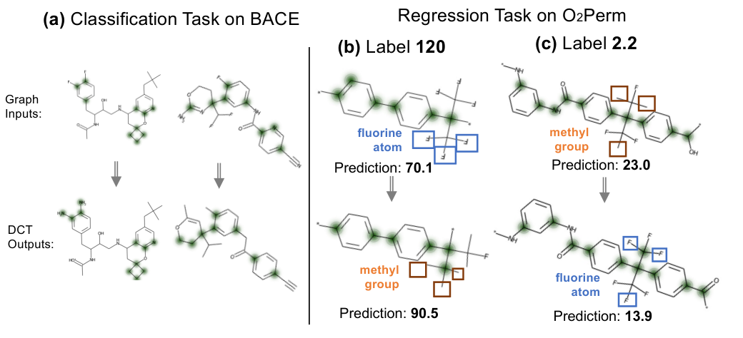
Knowledge transfer by data augmentation gives visible examples, allowing us to study what is learned. We visualize a few augmented graphs in DCT using ogbg-BACE and O2Perm. We adapt top-k pooling (Knyazev et al. 2019) to select the subgraphs that GIN used for prediction. The selected subgraphs are highlighted in green in fig. 6. The three examples show that the augmented graphs can identify and preserve the core structures that GIN uses to predict property values. These augmented graphs are chemically valid, showing that concepts such as some chemical rules from the unlabeled graphs are successfully transferred to downstream tasks. More results are in section D.2. Regarding task-specific knowledge, it is known that the fluorine atom and the methyl group are usually negatively and positively correlated to the permeability, respectively (Park et al. 2003; Corrado and Guo 2020). The augmented examples show that DCT captures this domain knowledge with the task-related objectives. In example (b), DCT replaces most of the fluorine atoms with the methyl groups. It encourages GIN to learn the positive relationship between the methyl group and the permeability so that GIN predicts a high label value. In example (c), DCT replaces the methyl groups with fluorine atoms. It encourages GIN to learn the negative relationship between the fluorine atom and the permeability so that GIN predicts a low label value.
5 Related Work
5.1 Graph Property Prediction
Graph neural networks (GNNs) (Kipf and Welling 2017; Xu et al. 2019) are commonly used for graph property prediction in chemistry and polymer informatics tasks (Otsuka et al. 2011; Hu et al. 2020; Zhou et al. 2022). However, it is hard to annotate enough labels in these domains. Recent work used self-supervised tasks such as node attribute prediction and graph structure prediction (Hu et al. 2019; You et al. 2021; Kim et al. 2022) to pre-train architecture-fixed GNNs. Sun et al. 2022 observed that the existing methods might fail to transfer knowledge from unlabeled graph data. Flexible GNN architectures for downstream tasks would be desirable.
Graph data augmentation (GDA) methods do not restrict GNN architecture choices to improve prediction accuracy (Trivedi et al. 2022; Zhao et al. 2022; Zhao et al. 2023; Ding et al. 2022). They learn to create new examples that preserve the properties of original graphs (Liu et al. 2022b; Liu et al. 2022a; Kong et al. 2022; Han et al. 2022; Luo et al. 2022). However, they purely manipulate labeled examples and thus cannot utilize the knowledge in unlabeled graphs. Our DCT combines the knowledge from the unlabeled dataset and the labeled task dataset. It creates label-preserved graph examples with the knowledge transferred from the unlabeled data. It allows the GNN models to have flexible architectures.
5.2 Learning from Unlabeled Data
Pre-training on self-supervised tasks such as masked image modeling and autoregressive text generation is effective for large language and vision models (Brown et al. 2020; He et al. 2022). However, the hand-crafted self-supervised tasks could hardly help models learn useful knowledge from unlabeled graphs due to the gap between these label-agnostic tasks and the downstream prediction tasks towards drug discovery and material discovery (Sun et al. 2021; Kim et al. 2022; Inae et al. 2023). A universal self-supervised task to learn from the unlabeled graphs remains under-explored (Sun et al. 2022; Trivedi et al. 2022).
Semi-supervised learning assumes that unlabeled and labeled data are from the same source (Liu et al. 2023). The learning objective in the latent space is usually mutual information maximization that encourages similarity between the representations of unlabeled and labeled graphs (Sun et al. 2020). However, the distributions of the unlabeled and labeled data could be very different due to the different types of sources (Hu et al. 2019), leading to negative impacts on the property prediction on the labeled graphs. Self-training, as a specific type of semi-supervised learning method, selects the unlabeled graphs of confidently predictable labels and assigns pseudo-labels for them (Lee et al. 2013; Iscen et al. 2019). Many studies have explored improving uncertainty estimation (Gal and Ghahramani 2016; Tagasovska and Lopez-Paz 2019; Amini et al. 2020) to help the model filter out noise for reliable pseudo-labels. Recently, pseudo-labels have been applied in imbalanced learning (Liu et al. 2023) and representation learning (Ghiasi et al. 2021). However, self-training is restricted to confidently predictable labels and may ignore the huge number of any other unlabeled graphs (Huang et al. 2022). Therefore, it cannot fully utilize the knowledge in the unlabeled graphs.
In contrast, our DCT employs a diffusion model to extract knowledge (as the diffusion and reverse processes) from all the unlabeled graphs. DCT represents the knowledge as task-specific labeled examples to augment the target dataset, instead of uninterpretable pre-trained model parameters. We note that self- or semi-supervised learning does not conflict with DCT, and we leave their combinations for future work.
5.3 Diffusion Models on Graphs
Recent works have improved the diffusion models on graphs (Niu et al. 2020; Jo et al. 2022; Vignac et al. 2022; Kong et al. 2023; Chen et al. 2023). EDP-GNN (Niu et al. 2020) employed score matching for permutation-invariant graph data distribution. GDSS (Jo et al. 2022) extended the continuous-time framework [6] to model node-edge joint distribution. DiGress (Vignac et al. 2022) used the transition matrix to preserve the discrete natures of the graph structure. GraphARM (Kong et al. 2023) introduced a node-absorbing autoregressive diffusion process. EDGE (Chen et al. 2023) focused on efficiently generating larger graphs. Instead of improving the generation performance of the diffusion model, our model builds on score-based diffusion models (Jo et al. 2022; Song et al. 2021) for predictive tasks, i.e., , graph classification and graph regression.
6 Conclusion
In this work, we made the first attempt to transfer minimal sufficient knowledge from unlabeled graphs by data augmentation. We proposed a data-centric framework to use the diffusion model trained on the unlabeled graphs and use two task-related objectives to generate task-specific augmented graphs. Experiments demonstrated the performance of the proposed framework through visible augmented examples. It is better than self-supervised learning, self-training, and graph data augmentation methods on as many as 15 tasks.
Acknowledgments and Disclosure of Funding
This work was supported by NSF IIS-2142827, IIS-2146761, IIS-2234058, CBET-2102592, and ONR N00014-22-1-2507.
References
- Amini et al. [2020] Alexander Amini, Wilko Schwarting, Ava Soleimany, and Daniela Rus. Deep evidential regression. Advances in Neural Information Processing Systems, 33:14927–14937, 2020.
- Antoniou et al. [2017] Antreas Antoniou, Amos Storkey, and Harrison Edwards. Data augmentation generative adversarial networks. arXiv preprint arXiv:1711.04340, 2017.
- Balestriero et al. [2022] Randall Balestriero, Leon Bottou, and Yann LeCun. The effects of regularization and data augmentation are class dependent. arXiv preprint arXiv:2204.03632, 2022.
- Böhm et al. [2004] Hans-Joachim Böhm, Alexander Flohr, and Martin Stahl. Scaffold hopping. Drug discovery today: Technologies, 1(3):217–224, 2004.
- Bowles et al. [2018] Christopher Bowles, Liang Chen, Ricardo Guerrero, Paul Bentley, Roger Gunn, Alexander Hammers, David Alexander Dickie, Maria Valdés Hernández, Joanna Wardlaw, and Daniel Rueckert. Gan augmentation: Augmenting training data using generative adversarial networks. arXiv preprint arXiv:1810.10863, 2018.
- Brown [2014] Nathan Brown. Bioisosteres and scaffold hopping in medicinal chemistry. Molecular informatics, 33(6-7):458–462, 2014.
- Brown et al. [2020] Tom Brown, Benjamin Mann, Nick Ryder, Melanie Subbiah, Jared D Kaplan, Prafulla Dhariwal, Arvind Neelakantan, Pranav Shyam, Girish Sastry, Amanda Askell, et al. Language models are few-shot learners. Advances in neural information processing systems, 33:1877–1901, 2020.
- Chen et al. [2023] Xiaohui Chen, Jiaxing He, Xu Han, and Li-Ping Liu. Efficient and degree-guided graph generation via discrete diffusion modeling. arXiv preprint arXiv:2305.04111, 2023.
- Cormack and Elorza [2004] Peter AG Cormack and Amaia Zurutuza Elorza. Molecularly imprinted polymers: synthesis and characterisation. Journal of chromatography B, 804(1):173–182, 2004.
- Corrado and Guo [2020] Tanner Corrado and Ruilan Guo. Macromolecular design strategies toward tailoring free volume in glassy polymers for high performance gas separation membranes. Molecular Systems Design & Engineering, 5(1):22–48, 2020.
- Cubuk et al. [2019] Ekin D Cubuk, Barret Zoph, Dandelion Mane, Vijay Vasudevan, and Quoc V Le. Autoaugment: Learning augmentation strategies from data. In Proceedings of the IEEE/CVF Conference on Computer Vision and Pattern Recognition, pages 113–123, 2019.
- Dhariwal and Nichol [2021] Prafulla Dhariwal and Alexander Nichol. Diffusion models beat gans on image synthesis. Advances in Neural Information Processing Systems, 34:8780–8794, 2021.
- Ding et al. [2022] Kaize Ding, Zhe Xu, Hanghang Tong, and Huan Liu. Data augmentation for deep graph learning: A survey. ACM SIGKDD Explorations Newsletter, 24(2):61–77, 2022.
- Gal and Ghahramani [2016] Yarin Gal and Zoubin Ghahramani. Dropout as a bayesian approximation: Representing model uncertainty in deep learning. In international conference on machine learning, pages 1050–1059. PMLR, 2016.
- Ghiasi et al. [2021] Golnaz Ghiasi, Barret Zoph, Ekin D Cubuk, Quoc V Le, and Tsung-Yi Lin. Multi-task self-training for learning general representations. In Proceedings of the IEEE/CVF International Conference on Computer Vision, pages 8856–8865, 2021.
- Han et al. [2022] Xiaotian Han, Zhimeng Jiang, Ninghao Liu, and Xia Hu. G-mixup: Graph data augmentation for graph classification. International Conference on Machine Learning, 2022.
- He et al. [2022] Kaiming He, Xinlei Chen, Saining Xie, Yanghao Li, Piotr Dollár, and Ross Girshick. Masked autoencoders are scalable vision learners. In Proceedings of the IEEE/CVF Conference on Computer Vision and Pattern Recognition, pages 16000–16009, 2022.
- Hu et al. [2019] Weihua Hu, Bowen Liu, Joseph Gomes, Marinka Zitnik, Percy Liang, Vijay Pande, and Jure Leskovec. Strategies for pre-training graph neural networks. arXiv preprint arXiv:1905.12265, 2019.
- Hu et al. [2020] Weihua Hu, Matthias Fey, Marinka Zitnik, Yuxiao Dong, Hongyu Ren, Bowen Liu, Michele Catasta, and Jure Leskovec. Open graph benchmark: Datasets for machine learning on graphs. Advances in neural information processing systems, 33:22118–22133, 2020.
- Huang et al. [2021] Kexin Huang, Tianfan Fu, Wenhao Gao, Yue Zhao, Yusuf H Roohani, Jure Leskovec, Connor W. Coley, Cao Xiao, Jimeng Sun, and Marinka Zitnik. Therapeutics data commons: Machine learning datasets and tasks for drug discovery and development. In Thirty-fifth Conference on Neural Information Processing Systems Datasets and Benchmarks Track, 2021.
- Huang et al. [2022] Kexin Huang, Vishnu Sresht, Brajesh Rai, and Mykola Bordyuh. Uncertainty-aware pseudo-labeling for quantum calculations. In The 38th Conference on Uncertainty in Artificial Intelligence, 2022.
- Inae et al. [2023] Eric Inae, Gang Liu, and Meng Jiang. Motif-aware attribute masking for molecular graph pre-training. arXiv preprint arXiv:2309.04589, 2023.
- Iscen et al. [2019] Ahmet Iscen, Giorgos Tolias, Yannis Avrithis, and Ondrej Chum. Label propagation for deep semi-supervised learning. In Proceedings of the IEEE/CVF conference on computer vision and pattern recognition, pages 5070–5079, 2019.
- Jo et al. [2022] Jaehyeong Jo, Seul Lee, and Sung Ju Hwang. Score-based generative modeling of graphs via the system of stochastic differential equations. In International Conference on Machine Learning, volume 162, pages 10362–10383. PMLR, 2022.
- Kashefi and Hwa [2020] Omid Kashefi and Rebecca Hwa. Quantifying the evaluation of heuristic methods for textual data augmentation. In Proceedings of the Sixth Workshop on Noisy User-generated Text (W-NUT 2020), 2020.
- Kim et al. [2022] Dongki Kim, Jinheon Baek, and Sung Ju Hwang. Graph self-supervised learning with accurate discrepancy learning. Advances in Neural Information Processing Systems, 2022.
- Kipf and Welling [2017] Thomas N Kipf and Max Welling. Semi-supervised classification with graph convolutional networks. In International Conference on Learning Representations, 2017.
- Knyazev et al. [2019] Boris Knyazev, Graham W Taylor, and Mohamed Amer. Understanding attention and generalization in graph neural networks. Advances in neural information processing systems, 32, 2019.
- Kong et al. [2022] Kezhi Kong, Guohao Li, Mucong Ding, Zuxuan Wu, Chen Zhu, Bernard Ghanem, Gavin Taylor, and Tom Goldstein. Robust optimization as data augmentation for large-scale graphs. In Proceedings of the IEEE/CVF Conference on Computer Vision and Pattern Recognition, pages 60–69, 2022.
- Kong et al. [2023] Lingkai Kong, Jiaming Cui, Haotian Sun, Yuchen Zhuang, B Aditya Prakash, and Chao Zhang. Autoregressive diffusion model for graph generation. International conference on machine learning, 2023.
- Lee et al. [2013] Dong-Hyun Lee et al. Pseudo-label: The simple and efficient semi-supervised learning method for deep neural networks. In Workshop on challenges in representation learning, ICML, volume 3, page 896. Atlanta, 2013.
- Liu et al. [2018] Bo Liu, Xudong Wang, Mandar Dixit, Roland Kwitt, and Nuno Vasconcelos. Feature space transfer for data augmentation. In Proceedings of the IEEE conference on computer vision and pattern recognition, pages 9090–9098, 2018.
- Liu et al. [2022a] Gang Liu, Tong Zhao, Jiaxin Xu, Tengfei Luo, and Meng Jiang. Graph rationalization with environment-based augmentations. Proceedings of the 28th ACM SIGKDD international conference on knowledge discovery & data mining, 2022a.
- Liu et al. [2023] Gang Liu, Tong Zhao, Eric Inae, Tengfei Luo, and Meng Jiang. Semi-supervised graph imbalanced regression. arXiv preprint arXiv:2305.12087, 2023.
- Liu et al. [2022b] Songtao Liu, Rex Ying, Hanze Dong, Lanqing Li, Tingyang Xu, Yu Rong, Peilin Zhao, Junzhou Huang, and Dinghao Wu. Local augmentation for graph neural networks. In International Conference on Machine Learning, pages 14054–14072. PMLR, 2022b.
- Luo et al. [2022] Youzhi Luo, Michael McThrow, Wing Yee Au, Tao Komikado, Kanji Uchino, Koji Maruhash, and Shuiwang Ji. Automated data augmentations for graph classification. arXiv preprint arXiv:2202.13248, 2022.
- Ma et al. [2022] Ruimin Ma, Hanfeng Zhang, Jiaxin Xu, Luning Sun, Yoshihiro Hayashi, Ryo Yoshida, Junichiro Shiomi, Jian-xun Wang, and Tengfei Luo. Machine learning-assisted exploration of thermally conductive polymers based on high-throughput molecular dynamics simulations. Materials Today Physics, 28:100850, 2022.
- Maziarka et al. [2020] Łukasz Maziarka, Agnieszka Pocha, Jan Kaczmarczyk, Krzysztof Rataj, Tomasz Danel, and Michał Warchoł. Mol-cyclegan: a generative model for molecular optimization. Journal of Cheminformatics, 12(1):1–18, 2020.
- Niu et al. [2020] Chenhao Niu, Yang Song, Jiaming Song, Shengjia Zhao, Aditya Grover, and Stefano Ermon. Permutation invariant graph generation via score-based generative modeling. In International Conference on Artificial Intelligence and Statistics, pages 4474–4484. PMLR, 2020.
- Oord et al. [2018] Aaron van den Oord, Yazhe Li, and Oriol Vinyals. Representation learning with contrastive predictive coding. arXiv preprint arXiv:1807.03748, 2018.
- Otsuka et al. [2011] Shingo Otsuka, Isao Kuwajima, Junko Hosoya, Yibin Xu, and Masayoshi Yamazaki. Polyinfo: Polymer database for polymeric materials design. In 2011 International Conference on Emerging Intelligent Data and Web Technologies, pages 22–29. IEEE, 2011.
- Park et al. [2003] Sang-Hee Park, Kwang-Je Kim, Won-Wook So, Sang-Jin Moon, and Soo-Bok Lee. Gas separation properties of 6fda-based polyimide membranes with a polar group. Macromolecular Research, 11:157–162, 2003.
- Poole et al. [2019] Ben Poole, Sherjil Ozair, Aaron Van Den Oord, Alex Alemi, and George Tucker. On variational bounds of mutual information. In International Conference on Machine Learning, pages 5171–5180. PMLR, 2019.
- Ramakrishnan et al. [2014] Raghunathan Ramakrishnan, Pavlo O Dral, Matthias Rupp, and O Anatole Von Lilienfeld. Quantum chemistry structures and properties of 134 kilo molecules. Scientific data, 1(1):1–7, 2014.
- Rong et al. [2019] Yu Rong, Wenbing Huang, Tingyang Xu, and Junzhou Huang. Dropedge: Towards deep graph convolutional networks on node classification. arXiv preprint arXiv:1907.10903, 2019.
- Rong et al. [2020] Yu Rong, Yatao Bian, Tingyang Xu, Weiyang Xie, Ying Wei, Wenbing Huang, and Junzhou Huang. Self-supervised graph transformer on large-scale molecular data. Advances in Neural Information Processing Systems, 33:12559–12571, 2020.
- Shorten and Khoshgoftaar [2019] Connor Shorten and Taghi M Khoshgoftaar. A survey on image data augmentation for deep learning. Journal of big data, 6(1):1–48, 2019.
- Soatto and Chiuso [2016] Stefano Soatto and Alessandro Chiuso. Visual representations: Defining properties and deep approximations. International Conference on Learning Representations, 2016.
- Song et al. [2021] Yang Song, Jascha Sohl-Dickstein, Diederik P Kingma, Abhishek Kumar, Stefano Ermon, and Ben Poole. Score-based generative modeling through stochastic differential equations. International Conference on Learning Representations, 2021.
- Sterling and Irwin [2015] Teague Sterling and John J Irwin. Zinc 15–ligand discovery for everyone. Journal of chemical information and modeling, 55(11):2324–2337, 2015.
- Sun et al. [2020] Fan-Yun Sun, Jordan Hoffmann, Vikas Verma, and Jian Tang. Infograph: Unsupervised and semi-supervised graph-level representation learning via mutual information maximization. International Conference on Learning Representations, 2020.
- Sun et al. [2021] Mengying Sun, Jing Xing, Huijun Wang, Bin Chen, and Jiayu Zhou. Mocl: data-driven molecular fingerprint via knowledge-aware contrastive learning from molecular graph. In Proceedings of the 27th ACM SIGKDD Conference on Knowledge Discovery & Data Mining, pages 3585–3594, 2021.
- Sun et al. [2022] Ruoxi Sun, Hanjun Dai, and Adams Wei Yu. Does gnn pretraining help molecular representation? Advances in Neural Information Processing Systems, 2022.
- Tagasovska and Lopez-Paz [2019] Natasa Tagasovska and David Lopez-Paz. Single-model uncertainties for deep learning. Advances in Neural Information Processing Systems, 32, 2019.
- Thornton et al. [2012] A Thornton, L Robeson, B Freeman, and D Uhlmann. Polymer gas separation membrane database, 2012.
- Tian et al. [2020] Yonglong Tian, Chen Sun, Ben Poole, Dilip Krishnan, Cordelia Schmid, and Phillip Isola. What makes for good views for contrastive learning? Advances in Neural Information Processing Systems, 33:6827–6839, 2020.
- Trivedi et al. [2022] Puja Trivedi, Ekdeep Singh Lubana, Mark Heimann, Danai Koutra, and Jayaraman J Thiagarajan. Analyzing data-centric properties for graph contrastive learning. In Advances in Neural Information Processing Systems, 2022.
- Velickovic et al. [2019] Petar Velickovic, William Fedus, William L Hamilton, Pietro Liò, Yoshua Bengio, and R Devon Hjelm. Deep graph infomax. ICLR (Poster), 2(3):4, 2019.
- Vignac et al. [2022] Clement Vignac, Igor Krawczuk, Antoine Siraudin, Bohan Wang, Volkan Cevher, and Pascal Frossard. Digress: Discrete denoising diffusion for graph generation. arXiv preprint arXiv:2209.14734, 2022.
- Wu et al. [2018] Zhenqin Wu, Bharath Ramsundar, Evan N Feinberg, Joseph Gomes, Caleb Geniesse, Aneesh S Pappu, Karl Leswing, and Vijay Pande. Moleculenet: a benchmark for molecular machine learning. Chemical science, 9(2):513–530, 2018.
- Xu et al. [2019] Keyulu Xu, Weihua Hu, Jure Leskovec, and Stefanie Jegelka. How powerful are graph neural networks? International Conference on Learning Representations, 2019.
- Xu et al. [2021] Minghao Xu, Hang Wang, Bingbing Ni, Hongyu Guo, and Jian Tang. Self-supervised graph-level representation learning with local and global structure. In International Conference on Machine Learning, pages 11548–11558. PMLR, 2021.
- You et al. [2021] Yuning You, Tianlong Chen, Yang Shen, and Zhangyang Wang. Graph contrastive learning automated. In International Conference on Machine Learning, pages 12121–12132. PMLR, 2021.
- Zhang et al. [2021] Zaixi Zhang, Qi Liu, Hao Wang, Chengqiang Lu, and Chee-Kong Lee. Motif-based graph self-supervised learning for molecular property prediction. Advances in Neural Information Processing Systems, 34:15870–15882, 2021.
- Zhao et al. [2021] Tong Zhao, Yozen Liu, Leonardo Neves, Oliver Woodford, Meng Jiang, and Neil Shah. Data augmentation for graph neural networks. In Proceedings of the aaai conference on artificial intelligence, volume 35, pages 11015–11023, 2021.
- Zhao et al. [2022] Tong Zhao, Gang Liu, Daheng Wang, Wenhao Yu, and Meng Jiang. Learning from counterfactual links for link prediction. In International Conference on Machine Learning, pages 26911–26926. PMLR, 2022.
- Zhao et al. [2023] Tong Zhao, Wei Jin, Yozen Liu, Yingheng Wang, Gang Liu, Stephan Günneman, Neil Shah, and Meng Jiang. Graph data augmentation for graph machine learning: A survey. IEEE Data Engineering Bulletin, 2023.
- Zhou et al. [2022] Kuangqi Zhou, Kaixin Wang, Jian Tang, Jiashi Feng, Bryan Hooi, Peilin Zhao, Tingyang Xu, and Xinchao Wang. Jointly modelling uncertainty and diversity for active molecular property prediction. In Learning on Graphs Conference, pages 29–1. PMLR, 2022.
Appendix A Additional Related Work on Data-Centric Approach
Data Augmentation
Data augmentation creates new examples with preserved labels but uses no unlabeled data [Shorten and Khoshgoftaar 2019, Kashefi and Hwa 2020, Balestriero et al. 2022]. Examples of heuristic data augmentation techniques include flipping, distorting, and rotating images [Shorten and Khoshgoftaar 2019], using lexical substitution, inserting words, and shuffling sentences in texts [Kashefi and Hwa 2020], and deleting nodes and dropping edges in graphs [Zhao et al. 2021, Zhao et al. 2023]. While human knowledge can be used to improve data diversity and reduce over-fitting in heuristic methods, it is difficult to use a single heuristic method to preserve the different labels for different tasks [Balestriero et al. 2022, Cubuk et al. 2019]. So, automated augmentation [Cubuk et al. 2019] learned from data to search for the best policy to combine a bunch of predefined heuristic augmentations. Generation models [Antoniou et al. 2017, Bowles et al. 2018, Han et al. 2022] create in-class examples. Other learning ideas such as FATTEN [Liu et al. 2018] and GREA [Liu et al. 2022a] learned to split the latent space for data augmentation. However, learning and augmenting from insufficient labels at the same time may limit the diversity of new examples and cause over-fitting. DCT leverages unlabeled data to avoid them.
Relationship between Data-Centric Approaches
As presented in fig. 7, perturb edges, delete nodes and mask attributes [Rong et al. 2019, Trivedi et al. 2022] for graphs are some heuristic ways for data augmentation. The augmented knowledge from them is mainly controlled by human prior knowledge on the perturbations and it often fails to be close to the task, i.e., , random perturbations hardly preserve labels for the augmented graphs. The learning to augment approaches learn from labeled graphs to perturb graph structures [Luo et al. 2022], to estimate graphons for different classes [Han et al. 2022], or to split the latent space for augmentation [Liu et al. 2022a]. Although these approaches could preserve labels for the augmented graphs, they introduce less extra knowledge to improve the model prediction. In summary, graph data augmentation is effective in expanding knowledge for limited labels, but it makes no use of unlabeled graphs. Besides, the diversity and richness of the domain knowledge from augmented graphs are far from that contained in a large number of unlabeled graphs. To learn from unlabeled graphs, data-centric approaches like the self-training is assumed to be useful when the unlabeled and labeled data are from the same source. It is less studied when we have a single unified unlabeled source for different tasks.
Appendix B Additional Method Details
B.1 Upper bounding the mutual information
In eq. 6, we use a leave-one-out variant of InfoNCE () to derive the upper bound of mutual information. We summarize the derivation [Poole et al. 2019] here.
| (9) |
The intractable upper bound is minimized when the variational approximation matches the true marginal [Poole et al. 2019]. For each , its augmented output , and negative examples with different labels, we could approximate . So, we have
| (10) |
B.2 Extraction of Statistical Features on Graphs
For each molecule and polymer graph, we concatenate the following vectors or values for statistical feature extraction.
- •
the sum of the degree in the graph;
- •
the vector indicating the distribution of atom types;
- •
the vector containing the maximum, minimum and mean values of atoms weights in a molecule or polymer;
- •
the vector containing the maximum, minimum, and mean values of bond valence.
For each protein-protein interaction ego-graph in the biology field, we use the sorted vector of node degree distribution in the graph as the statistical features.
B.3 Technical Details for Graph Data Augmentation with Diffusion Model
The Lookup Table from Atom Type to Node Embedding Space
Given a graph , we assume the node feature matrix on the graph is , where is the number of nodes. The edge feature matrix is , where is the number of edges. There are two ways for to represent the graph structure in practice. We can use either the dense adjacency matrix or sparse edge index . The diffusion model [Jo et al. 2022] on graphs prefers the former, which is more straightforward for graph generations. The prediction model prefers the latter because of its flexibility, and less computational cost and time. The transformation between two types of graph structure representation takes additional time. Particularly for molecular graphs, the node features used for generation (one-hot encoding of the atom type) and for prediction (see the official package of OGBG 11 1 https://github.com/snap-stanford/ogb/blob/master/ogb/utils/features.py for details) are different, which introduces extra time to process the graph data. For details, we (1) first need to extract discrete node attributes given the atom type and its neighborhoods; (2) we then need to use an embedding table to embed node attributes in a continuous embedding space; (3) the embedding features of nodes with their graph structure are inputted into the graph neural networks to get the latent representation for nodes. The reverse process for data augmentation in DCT may need to repeatedly process graph data with steps (1) and (2). It introduces additional time. To address these technical problems, we build up a lookup table to directly map the atom type to the node embedding. We average the node attributes for the same type of node within the batch. We then use the continuous node attributes as weights to average the corresponding node embedding according to the table.
Instantiations of SDE on Graphs
According to Song et al. 2021, we use the Variance Exploding (VE) SDE for the diffusion process. Given the minimal noise and the maximal noise , the VE SDE is:
| (11) |
The perturbation kernel is derived [Song et al. 2021] as:
| (12) |
On graphs, we follow Jo et al. 2022 to separate the perturbation of adjacency matrix and node features:
| (13) |
The Sampling Algorithm in the Reverse Process for Graph Data Augmentation
We adapt the Predictor-Corrector (PC) samplers for the graph data augmentation in the reverse process. The algorithm is shown in algorithm 1.
The Algorithm of the Framework
The algorithm of the proposed data-centric knowledge transfer framework is presented in algorithm 2 and algorithm 3. In detail, algorithm 2 corresponds to section 3.2 and algorithm 3 corresponds to section 3.3.
Appendix C Additional Experiments Set-ups
We perform experiments on 15 datasets, including eight classification and seven regression tasks from chemistry, material science, and biology. We use Area under the ROC curve (AUC) for classification performance and mean absolute error (MAE) for regression.
C.1 Molecule Classification and Regression Tasks
Seven molecule classification and three molecule regression tasks are from open graph benchmark [Hu et al. 2020]. They were originally collected by MoleculeNet [Wu et al. 2018] and used to predict molecule properties. They include (1) inhibition to HIV virus replication in ogbg-HIV, (2) toxicological properties of 617 types in ogbg-ToxCast, (3) toxicity measurements such as nuclear receptors and stress response in ogbg-Tox21, (4) blood–brain barrier permeability in ogbg-BBBP, (5) inhibition to human -secretase 1 in ogbg-BACE, (6) FDA approval status or failed clinical trial in ogbg-ClinTox, (7) having drug side effects of 27 system organ classes in ogbg-SIDER, (8) predicting the property of lipophilicity in ogbg-Lipo, (9) predicting the water solubility ( solubility in mols per litre) from chemical structures in ogbg-ESOL, (10) predicting the hydration free energy of molecules in water in ogbg-FreeSolv. For all molecule datasets, we use the scaffold splitting procedure as the open graph benchmark adopted [Hu et al. 2020]. It attempts to separate structurally different molecules into different subsets, which provides a more realistic estimate of model performance in experiments [Wu et al. 2018].
C.2 Polymer Regression Tasks
Four polymer regression tasks include GlassTemp, MeltingTemp, ThermCond, and O2Perm. They are used to predict different polymer properties such as glass transition temperature (∘C), melting temperature (∘C), thermal conductivity (W/mK) and oxygen permeability (Barrer). GlassTemp and MeltingTemp are collected from PolyInfo, which is the largest web-based polymer database [Otsuka et al. 2011]. The ThermCond dataset is from molecular dynamics simulation and is an extension from the dataset used in [Ma et al. 2022]. The O2Perm dataset is created from the Membrane Society of Australasia portal, consisting of a variety of gas permeability data [Thornton et al. 2012]. Since a polymer is built from repeated units, researchers often use a single unit graph with polymerization points as polymer graphs to predict properties. Different from molecular graphs, two polymerization points are two special nodes (see “” in fig. 2), indicating the polymerization of monomers [Cormack and Elorza 2004]. For all the polymer tasks, we randomly split by 60%/10%/30% for training, validation, and test.
C.3 Protein Classification Task
An additional task is protein function prediction using protein-protein interaction graphs [Hu et al. 2019]. A node is a protein without attributes, an edge is a relation type between two proteins such as co-expression and co-occurrence. In our DCT, we treat all the relations as the undirected edge without attributes.
C.4 Baselines and Implementation
When implementing GIN [Xu et al. 2019], we tune its hyper-parameters for different tasks with an early stop on the validation set. We generally implement pre-training baselines following their own setting. For molecule and polymer property prediction and protein function prediction, the pre-trained GIN models with self-supervised tasks such as EdgePred, AttrMask, ContextPred in [Hu et al. 2019], InfoMax [Velickovic et al. 2019] are available. So we directly use them. For other self-supervised methods, we implement their codes with default hyper-parameters. Following their settings, we use 2M ZINC15 [Sterling and Irwin 2015] to pre-train GIN models for molecule and polymer property prediction. We use 306K unlabeled protein-protein interaction ego-networks [Hu et al. 2019] to pre-train the GIN for the downstream protein function property prediction. For self-training with real unlabeled graphs and InfoGraph [Sun et al. 2020], we use 113K QM9 [Ramakrishnan et al. 2014]. For self-training with generated unlabeled graphs, we train the diffusion model [Jo et al. 2022] on the real QM9 dataset and then produce the same number of generated unlabeled graphs. To train the diffusion model in our DCT, we also use QM9 [Ramakrishnan et al. 2014].
Appendix D Additional Experiment Analysis
D.1 The Power of Diffusion Model to Learn from Unlabeled Graphs
In table 3, when we replace the 133K QM9 with the 249K ZINC [Jo et al. 2022] to train the diffusion model, which nearly doubles the size of the unlabeled graphs and includes more atom types, we do not observe any additional improvement, and in some cases, even worse performance. It is possible because of the constraint of the current diffusion model’s capacity to model the data distribution for a much larger number of more complex graphs. It encourages powerful generative models in the future, which could be directly used to benefit predictive models under the proposed framework.
D.2 Chemical Validity of the Generated Graphs in Downstream Tasks
In fig. 6, we show through some examples that concepts, such as certain chemical rules from the unlabeled graphs, are successfully transferred to downstream tasks. To further validate this point, we gathered 1,000 task-specific graphs generated in the intermediate steps on the tasks of ogbg-BACE, ogbg-BBBP, ogbg-FreeSolv, and O2Perm. We then assessed the chemical validity of these graphs and observed that the validity is 92.8%, 87.9%, 97.4%, and 62.1%, respectively. Results show that transferring knowledge from pre-trained molecular data to target molecules yields relatively high chemical validity. However, the validity drops to 62% when transferring knowledge from pre-trained molecular data to target polymer data. This finding indicates that the transferability of chemical rules becomes more challenging when the distribution gap between the pre-training data and downstream task data is larger.