Experimental verification of an online traction parameter identification methodJournal: Control Engineering Practice
Abstract
Traction parameters, that characterize the ground-wheel contact dynamics, are the central factor in the energy efficiency of vehicles. To optimize fuel consumption, reduce wear of tires, increase productivity etc., knowledge of current traction parameters is unavoidable. Unfortunately, these parameters are difficult to measure and require expensive force and torque sensors. An alternative way is to use system identification to determine them. In this work, we validate such a method in field experiments with a mobile robot. The method is based on an adaptive Kalman filter. We show how it estimates the traction parameters online, during the motion on the field, and compare them to their values determined via a 6-directional force-torque sensor installed for verification. Data of adhesion slip ratio curves is recorded and compared to curves from literature for additional validation of the method. The results can establish a foundation for a number of optimal traction methods.
Keywords:
System identification , Kalman filter , Vehicle Dynamics , Traction1 Introduction
Tractors have a huge market share that is steadily growing throughout the world (Global Industry Analyst 2019). Machines with less than 30 HP alone are expected to grow by 60.7 Billion dollars until 2025. However, fuel costs and environmental regulations put ever stronger requirements on productivity and energy efficiency of such heavy-duty vehicles. Productivity and energy efficiency in turn are highly dependent on ground conditions, which are usually unknown and change dynamically. Determining traction parameters requires knowledge of wheel-ground forces which can be measured by relatively expensive sensors. Online identification is an alternative way and is investigated experimentally in this work.
Energy efficiency characterizes the amount of driving power actually transmitted into pulling, whereas productivity is the ground speed times the working area. Working area refers to width in case of tillage or depth times width in case of bulldozing. The key traction parameters thereby are the adhesion and the rolling resistance coefficients. They are the gross pulling force and, respectively, rolling resistance normalized by the vertical load. Both are functions of the wheel slip ratio. See Fig. 1 for typical energy efficiency and adhesion coefficient depending on slip ratio. The reader may refer to the classical work of (Söhne 1964) for a detailed description of traction slip ratio characteristics on different soils. The overall operation performance can be understood in terms of balancing propulsion and energy efficiency and requires knowledge of the adhesion slip ratio curve (see Fig. 1) as well as the rolling resistance coefficient.

Various models describing soil-wheel interaction have been developed, the approaches range from empirical to semi-empirical to finite element models. Some are reviewed here. Wismer and Luth 1973 and Brixius 1987 developed empirical models to predict traction performance using soil properties and tire parameters. Their methods have found application in various works, e. g. Kim and Lee 2018 who used it in a slip controller. Sandu et al. 2011 developed a semi-empirical off-road tire model for soft soil application which improves on existing models by providing a more detailed modeling of the soil-wheel contact surface. Rajamani et al. 2012 developed observers to estimate friction coefficients of individual wheels during operation from various measurements, e. g. engine torque, brake torque and GPS measurements. The topic keeps attracting attention of researches in recent time – Pentos and Pieczarka 2017 used an artificial neural network to predict the influence of the soil texture, soil moisture, compaction etc. on the propulsion force and traction efficiency. Alexander et al. 2018 proposed using a data buffer coupled with a parameter fit algorithm for traction optimization. Cook et al. 2019 recently developed a method for controlling tracked vehicles, where propulsion force, drive torque and slip ratio are estimated and compared to a list of known terrain traction models to find a suitable slip ratio set point.
This work will make use of Kalman filter based methods of traction identification. Turnip and Fakhrurroja 2013 used an identification approach based on the extended Kalman filter (EKF), whereas Hamann et al. 2014 suggested to use a superior variant of the EKF – the unscented Kalman filter (UKF), see (Wan and Van Der Merwe 2000; Van Der Merwe et al. 2004). For an extensive review of wheel-soil-interaction models, traction parameter estimation, traction control schemes and wheel slip ratio estimation refer to (Sunusi et al. 2020).
It is clear that the topic raised in this work is of high relevance and the reported results here contribute to the problem of online traction parameter identification. In the following, we outline briefly the approach.
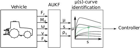
First of all, in a previous work (Kobelski et al. 2020) an UKF-based identification algorithm was used to estimate traction properties of a tractor driving over different ground types in a simulation. It was based on the methodology developed in (Osinenko et al. 2014; Osinenko et al. 2016; Osinenko and Streif 2017). In (Osinenko et al. 2016) the adaptive unscented Kalmanfilter with a fuzzy supervisor was used to assist traction control, while (Osinenko and Streif 2017) improved the model for the adhesion slip ratio characteristic curves. This work follows up by validating the previously derived concept experimentally. The goal of this work is to evaluate the tracking capabilities of the UKF under experimental conditions, record adhesion slip ratio curves for different soils and to test whether a change in ground conditions can be detected by the UKF. A model for longitudinal motion dynamics based on dynamical equations combined with an adaptive UKF is used for the identification of the ground traction properties, namely, the adhesion coefficient and the soil deformation rolling resistance coefficient . These two parameters are of the essence during slip control as they heavily influence productivity and energy efficiency, see Fig. 1. Fig. 2 shows a schematic of the overall algorithm. The experimental design will be explained in detail, including the test vehicle with its sensor setup and the experimental site. Statistical evaluation of the proposed algorithm is provided.
2 Materials and Methods
In this section, firstly, a model for the longitudinal motion dynamics of a vehicle derived from standard Newton equations is given. An empirical model for adhesion slip ratio characteristics is introduced afterwards. Then, the applied adaptive unscented Kalman filter is described. In the last part, the design and setup of validation experiments is described.
2.1 Motion dynamics

Model equations are derived in a similar fashion as in Kobelski et al. 2020. Consider the wheel force diagram of Fig. 3. There, the driving torque exerts a horizontal force distribution in the contact area that can be summarized in a single force . The reaction of the vehicle’s body is exerted in the opposite direction of . The wheel-ground contact results in the deformation of the tire and soil respectively, which in turn results in a tire deformation rolling resistance force as well as a soil deformation rolling resistance force , with their respective rolling resistance coefficients and . The bearing friction is assumed proportional to the revolution speed with the resistance coefficient . The dynamical rolling radius describes the deformed tire’s distance between its center and ground. The vertical (or normal) force equals the sum of the axle load and wheel weight plus the vertical inertia force. Due to the tire and soil deformation, the point of application of the soil reaction forces is shifted by . By convention, the term is assumed to be equal , where , i. e. the tire-deformation rolling resistance. The force and and torque balance equations read:
| (1) | ||||
| (2) |
Here, is the wheel mass, is the ground speed and is the wheel moment of inertia. The total rolling resistance off-road is dominated by the soil-deformation resistance and significantly influences the energy efficiency. The soil deformation rolling resistance is summarized into . With (1) the longitudinal dynamics for the whole vehicle now are
| (3) |
where is the vehicle mass, is the horizontal part of the drawbar pull, i. e. the implement resistance and is the wheel index.
Dividing the horizontal force by the vertical force yield the adhesion coefficient
| (4) |
The part of the horizontal force that actually drives the wheel forward is called net traction ratio
| (5) |
The following definition of slip ratio is used:
| (6) |
It ranges from -1 (locked wheel) to 1 (spinning on the spot). The energy efficiency is defined by the formula:
| (7) |
Note that , and are functions of the slip ratio .
The tire deformation resistance mainly depends on tire type and inflation pressure and can therefore be estimated prior to operation, while the soil deformation resistance and will be estimated using a state observer. Due to vertical forces the wheel is deformed which reduces the rolling radius dynamically. Please refer to (Guskov et al. 1988, p.40) for an empirical formula for estimation of the rolling radius .
The parameters , , and are assumed known. For details on estimation of and , please refer to (Osinenko et al. 2015).
2.2 Adhesion Slip Ratio Characteristic Model
As was stated above, the adhesion coefficient is a function of the slip ratio (Fig. 1). It was observed from literature, e. g. Söhne 1964, that the shape of the adhesion-slip-curve (-curve) is similar for similar ground types.
There exists a variety of -curve models, e. g. (Pacejka 2006; Schreiber and Kutzbach 2007) . The empirical model from (Schreiber and Kutzbach 2007) is used as a basis in this work. The equation was first modified in (Osinenko et al. 2014) by replacing a linear term with an exponential one und further refined in (Osinenko and Streif 2017), by reducing the number of parameters by one:
| (8) |
Here, are the model parameters. For similar ground types the three parameters may be fixed, while only the parameter can be varied to cover a spectrum of ground conditions – see Fig. 5 in (Kobelski et al. 2020).
The -characteristics for each soil type can partially be obtained from literature, even before operation. However, data recorded during operation may be more accurate due to varying local circumstances such as moisture, tilling or soil composition. Hence, first a prototype -curve is fitted to data from literature using a graphical fitting tool, see Fig. 4. This gives parameters from Eq. (8). The last parameter is then identified for every soil type encountered in the experiments separately through a least square (LS) fit to recorded data. The identified curves are then evaluated statistically by comparing the identified -curves to recorded data, see section 3.2. There the model choice of Eq. 8 is also validated by experimental data.
Data from (Wünsche 2005) is used for the identification of the -prototype, see Fig. 4. Fitting all four parameters of Eq. (8) is a non convex problem and will not result in a unique solution. The graphical fitting tool allows the user to shape the prototype to fit well established data from literature or to self recorded data from experiments. The downside, however, is that the shape forming is highly subjective to the user. The next section explains, how the AUKF-FS identifies , and .

2.3 Adaptive Unscented Kalman filter
The identification algorithm used in this work bases on the AUKF suggested in (Zhe Jiang et al. 2007). The method has been throughly explained in previous work, while in this work only a basic understanding of its application is given (please refer to (Osinenko and Streif 2017) for a detailed explanation).
The adhesion coefficient impacts vehicle performance the most and knowledge of it is required for efficient traction control. For its identification, an adaptive UKF with a fuzzy-logic supervisor (AUKF-FS) is used. Its purpose is to estimate the state from the measured output . The generic model description behind the UKF reads:
| (9) | ||||
Here, is the state vector, is the input vector, is the output vector, is the non–linear state model, is the measurement model, are the state and measurement random noises with zero mean and covariance and respectively, denotes the normal probability distribution, is the time step index, are dimensions. The AUKF algorithm can be divided into two steps: prediction and update. The particular feature of the unscented Kalman filter is the calculation of the so called sigma-points for the prediction step. The sigma-points are able to capture the posterior mean and covariance after propagation through the system up to the 3rd order of a Taylor series linearization (please refer to (Wan and Van Der Merwe 2000) for details). In the second part of the prediction the UKF computes the estimate probability distribution using the sigma-points as follows:
| (10) |
In (10), is the a priori estimate covariance, and are the sigma–points with the weights . The predicted mean is computed from the sigma–points by the formula:
The a priori estimate covariance is calculated as follows:
| (11) |
where are weight factors.
The update step involves recalculating the sigma–points from . The mean of the predicted output
and covariance
as well as the state and output covariance,
are then used to calculate the Kalman gain . The last step is to update estimate mean with
| (12) |
and the a posteriori covariance now becomes
| (13) |
The choice of noise covariance is crucial – a poor choice of may result in divergence issues or noisy estimates (Fitzgerald 1971). The standard UKF was hence modified by adding an adaption matrix which replaces the state noise with (for an extensive description, please refer to (Osinenko et al. 2014)). The adaption matrix minimizes the difference between true measurements and measurement estimate, which helps avoiding divergence issues, however the estimates may become too noisy. To balance out these effects, it was suggested to introduce a fuzzy-logic system (FLS) to supervise the UKF. The FLS captures intensity of vehicle dynamics using difference equations for measurements of and over a moving window (please refer to Osinenko et al. 2016 for details). If the vehicle enters a phase of intense dynamics, the FLS factor is set high which gives priority to the adaptation matrix and prevents divergence. At steady phases, the FLS is set smaller, which reduces estimation noise. The resulting filter is called AUKF-FS (refer to (Osinenko and Streif 2017) for details).
From the vehicle dynamics model of Section 2.1 the state vector for the AUKF-FS consists of wheel speed , vehicle speed , adhesion coefficient and soil deformation rolling resistance .
The wheel speeds and vehicle ground speed form the output vector:
The input vector includes the drive torques, front vertical force and longitudinal component of the drawbar pull:
In (Kobelski et al. 2020) observability of the overall system as well as possibilities to measure or estimate , and are discussed. The tire deformation rolling resistance coefficients are assumed as fixed parameters. Propagation of the sigma-points through the system formed by Eq. (1) and (2) is performed using fourth-order Runga-Kutta method. It is assumed that the unknown parameters do not change during one integration step so that their dynamics are neglected.
2.4 Experiment Design
A mobile robot sensor platform was used to evaluate concepts of this work experimentally. In this section first the mobile robot, tools and the experimental site will be described. Afterwards experiments will be explained.

2.4.1 Tools and Experimental Site
The mobile robot used is a customized version of the Innok Robotics Heros 444. Its electric motors have a combined power of 1.6 kW, and each can be driven separately. The wheels have a diameter of 40 cm and the vehicle weighs 139 kg, weight balance is 54 kg on the front and 85 kg on the rear axis. It is equipped with a raspberry pi3 which functions as its brain, a NVIDIA Jetson TX2 for image processing and a LTE-WLAN-router. It is equipped with a multitude of sensors:
- 1.
Stereolabs ZED stereo camera for visual odometry
- 2.
GPS Trimble BX982
- 3.
wheel odometry
- 4.
motor torque from electric motors
- 5.
inertia measurement unit XSens MTi-30-AHRS- 2A5G4
- 6.
force and torque sensor K6D80 at the back right wheel axis
- 7.
force sensor KM30z to measure drawbar pull force
The robot is controlled with a remote controller during the experiments. Wheel revolution speed can be adjusted with a rotatory switch. In-built controllers ensure same revolution speed on all wheels.

Various tools, see Fig. 6, were connected to the mobile robot’s drawbar during the experiments. Another tool, used in the experiments, is a heavy steel frame, similar to the one surrounding the smooth surface roller in Fig. 6. Due to its structure, it could dig into the ground, which provided additional resistance during the experiments. Pulling different tools across ground surfaces causes different horizontal forces. Recall Eq. (4), diverse horizontal forces translate to a wide range of operation points that can be recorded.
Experiments were performed at a test site in Dresden, Germany. The soil in this region is mostly a sandy loam with pseudogley (soil value 69). The afore mentioned agricultural tools were used for experiments. Moisture and tillage of test sites could be adjusted to perform experiments on different ground types. Two separate test sites were provided for experiments. On the first field only one firmly pressed ground was present. On the second field three ground types were prepared. This is a list of soil types encountered in the experiments:
- hard
firm soil which provides good traction, only on the first field
- fine
tilled soil, relatively loose
- wet
same soil as fine, but moisturized for three hours with a sprinkler
- coarse
more coarse and uneven than fine with numerous earth clumps
- grass
short grass (less than 5 cm) is growing around the fields
See Fig. 7 for pictures of the different ground types.

2.4.2 Description of Experiment
Experimental data were stored on a Raspberry Pi and simultaneously transmitted to a laptop where it could be monitored in a Matlab/Simulink environment. Experiments were conducted by driving the mobile robot with one or more tools connected to the drawbar over the various soil types. 68 experiments were conducted in total. Some experiments were conducted by driving over the same soil type with different speeds while others involve driving over switching ground types. Note that the transition between two ground types is only finished when both the mobile robot and the pulled tool(s) are on the next ground. This has to be kept in mind for evaluation as data recorded during the transitioning period are not representing the respective ground type. Different combinations of tools as well as different wheel revolution speeds were tried during experiments, to receive data at multiple operation points on various soils. Two experiments - they will be referred to in the following as ’multi1’ and ’multi2’ - involve driving over multiple ground types during one experiment, see Fig. 8. These two particular experiments will be used to evaluate the UKF’s ability to estimate .

3 Results and discussion
The experiments had three main objectives. The first objective was to test the UKF’s ability to estimate . The second was to record -characteristics for different soils. The third objective was to determine whether soil types can be distinguished trough UKF estimates during operation. This is a prerequisite for future classification during operation, i. e. matching the underground to known ground types.
3.1 UKF Traction Estimation
The two experiments ’multi1’ and ’multi2’ will be used as a benchmark to evaluate the UKF’s tracking ability. The UKF estimate for will be henceforth called . Adhesion coefficient is calculated through Eq. (4) and from measurements of and at the rear right wheel.

Fig. 9 shows recorded versus during ’multi2’. At a few points differs significantly from . At 250 seconds there is a wide gap between and , which is caused by the vehicle getting stuck in the ’coarse’ soil. Due to its inertia, the tool connected to the vehicle would slide closer to the stuck vehicle. The tool now pushes against the vehicle, resulting in negative or very small and , while motor torque – which is the basis for the UKF estimate – and are high. Similar phenomena occured around 280 to 310 seconds and 450 seconds. On coarse soil the robot would get stuck or drive over large earth clumps, resulting in uneven loads for the axes. Data between 245 and 255 seconds are regarded as outliers and will be ignored during statistical evaluation. Without outliers, is 0.85 and normalized root mean square error (NRMSE) is 0.09. The root mean square error is normalized by the difference between maximum and minimum value of the observations. The overall performance is comparable to earlier works, see (Osinenko et al. 2014) and (Osinenko et al. 2016).
3.2 Soil Characteristic Identification

In section 2.2 a model, see Eq. (8), for the adhesion slip ratio curve was given. Using data from literature and a graphical fitting tool, a prototype curve was found. In this section a scaling factor for the prototype curve will be fit to data from experiments. This will validate the choice of the prototype curve and give different adhesion slip ratio curves for the soil types encoutered in the experiments.
| Hard | Fine | Wet | Coarse | Grass | |
| NRMSE | 0.046 | 0.093 | 0.138 | 0.088 | 0.15 |
| R2 | 0.975 | 0.9 | 0.76 | 0.91 | 0.84 |
| 1.42 | 0.85 | 0.83 | 0.91 | 0.4 |
From the experiments described in section 2.4 five types of soil can be extracted, i. e. ’hard’, ’fine’, ’coarse’, ’wet’ and ’grass’. For the purpose of curve fitting recorded data are summarized in ’bins’, where every ’bin’ stores data from a certain slip range, e. g. to , to etc. Data below 5% and above 60% slip ratio are neglected for fitting. For each bin, mean and standard deviation of are calculated, similar to a boxplot. Curves are fit to the mean of each bin instead of the whole point cloud. Fig. 10 shows the resulting fit for experiments on ’hard’. A visual comparison indicates a reasonably good fit, NRMSE and R2 are 0.046 and 0.975 respectively. Fig. 11 shows fitting for other soil types. For the soil ’grass’ only values up to 0.4 slip ratio were used, measurements above 0.4 slip ratio were very few and were hence considered outliers. Statistical evaluation is given in Table 1.
The soil types ’fine’ and ’wet’ can hardly be distinguished from each other, neither by comparing identified parameters ( versus ) nor by comparing their standard deviations. The identified parameter for ’coarse soil’ is similar to the previous two (), however data show significantly higher standard deviation. ’Grass’ shows overall a lower resulting in a lower parameter (). Furthermore, recorded data agree reasonably well with models from literature and with the model from Eq. (8).

3.3 Ground Change Detection
This section examines whether differences in soil type can be observed from and during operation. Data from experiments ’multi1’ and ’multi2’ is used as a benchmark for this. Recall that these were the two experiments, where the vehicle drove over multiple soil types. Data are split into different sections, where cutting points are the transition zones between soil types, e. g. from Fig. 8 it can be seen that ’multi1’ had three ’fine’ sections, three ’coarse’ sections etc. For each section, where the vehicle drives over a single soil type, data are summarized in a mean and standard deviation value for and respectively. Additionally UKF estimates are compared to measurements.


Fig. 12 shows mean and standard deviation of and for various soil type sections during the two experiments. Grass can easily be distinguished from the other soil types, as it has overall smaller and . On coarse soil the vehicle had slightly higher compared to fine and wet soil, however slip ratio mean and standard deviation are much higher. Wet and fine soil can be distinguished from grass and coarse soil, however no difference between fine and wet can be reliably recognized from these experiments. Perhaps the traction dynamics on these particular two soil types are too similar.
Fig. 13 compares mean and standard deviation from measurements to UKF estimates. Differences between and for ’grass’, ’wet’ and ’fine’ are smaller than 0.015, for ’coarse’ mean of and difference is 0.03, i. e. 8% of . It can be concluded that a shift in operation point can be observed in the -characteristic, even from UKF estimates. Therefore, distinguishing between soils during operation is plausible.
4 Conclusion
Knowledge of traction parameters is essential when deriving control strategies for heavy-duty vehicles such as tractors. Previous methods either involved offline estimation of said parameters, which has the downside of being less accurate due to dynamically changing conditions such as soil moisture or tilling, or required special and expensive measurements. The method developed in this work does not require special sensors to work and adapts to changing conditions during operation.
Traction parameters are estimated using an adaptive unscented Kalman filter. Then single measurements around a slip ratio operation point are used to estimate complete characteristic curves over a bandwidth of slip ratios. These characteristic curves can then be used in control to derive strategies that balance energy efficiency, productivity and tire wearing. In this work such a parameter estimation and curve identification algorithm was implemented on a mobile robot to verify the functionality in experiments.
Experiment evaluation shows reasonably good tracking capabilities of the AUKF estimation with . Earlier works, see (Osinenko et al. 2014) and (Osinenko et al. 2016), showed similar results for their simulations. Furthermore, identified adhesion slip ratio curves fit reasonably well to recorded experiment data, with ranging from to . In the last part of experiment evaluation it was tested, whether ground types are distinguishable during operation. It showed, that indeed most soils can be distinguished from each other – even with AUKF estimates – with the exception of ’wet’ and ’fine’. The reason for that is most likely because compared to a tractor the mobile robot was much smaller and light weighted, hence its wheel would not dig as deep into the soil as a real tractor would. The ’wet’ soil hence did not impede vehicle movement as much as expected. Overall it can be said, that a change of soil can be detected using this works AUKF estimation. The results can be used in different ways. The AUKF estimator is an easy and cheap to implement and works online during operation. Knowledge of adhesion slip characteristics is essential for control and hence there is potential to improve energy efficiency and productivity of tractors. Since operation points switch between soils with different traction properties, the underground may be identified and mapped using AUKF and Global Positioning System (GPS) information. This can also be used to detect anomalies in the underground, e. g. high may indicate firm soil which requires more tilling or patches of land where crops are growing more or less dense.
Future work will focus on the classification of soil types and ground recognition. It will be tested whether the driving surface can reliably be identified using this works AUKF estimates.
Decleration of competing interest
None declared.
Acknowledgments
This research was founded by the Saxon Ministery of Science and Art and the ’Sächsische Aufbaubank (SAB)’, SAB-project number 100333816. For technical support we acknowledge the Saxon State Office for Environment, Agriculture and Geology. We also would like to thank Christian Kröling for his excellent support in the realization of the field tests and the selection of the field equipment.
References
- Alexander et al. (2018) Alexander, A., Sciancalepore, A., Vacca, A., 2018. Online Controller Setpoint Optimization for Traction Control Systems Applied to Construction Machinery, in: Fluid Power Systems Technology.
- Brixius (1987) Brixius, W., 1987. Traction prediction equations for bias ply tires. ASAE Paper 87, 162.
- Cook et al. (2019) Cook, J.T., Ray, L.E., Lever, J.H., 2019. Mobility Enhancement of Heavy-Duty Tracked Vehicles Under Load Using Real-Time Terrain Characterization, Traction Control, and a Towing Winch. Journal of Dynamic Systems, Measurement, and Control 141.
- Fitzgerald (1971) Fitzgerald, R., 1971. Divergence of the Kalman filter. IEEE Transactions on Automatic Control 16, 736–747.
- Global Industry Analyst (2019) Global Industry Analyst, 2019. Global Farm Tractors Industry.
- Guskov et al. (1988) Guskov, V.V., Velev, N.N., Atamanov, Y.E., Bocharov, N.F., Ksenevich, I.P., Solonsky, A.S., 1988. Traktory: Teoriya: Uchebnik dlya Studentov Vuzov, po Specialnosti "Avtomobili i Traktory". [Tractors. Theory. Textbook for Students of Higher Educational Insitutions Majoring in Automotive and Tractor Technology (in Russian)]. Moscow: Mashinostroenie.
- Hamann et al. (2014) Hamann, H.F., Hedrick, J.K., Rhode, S., Gauterin, F., 2014. Tire force estimation for a passenger vehicle with the unscented kalman filter, in: Intelligent Vehicles Symposium Proceedings, 2014 IEEE, IEEE. pp. 814–819.
- Kim and Lee (2018) Kim, J., Lee, J., 2018. Traction-energy balancing adaptive control with slip optimization for wheeled robots on rough terrain. Cognitive Systems Research 49, 142 – 156.
- Kobelski et al. (2020) Kobelski, A., Osinenko, P., Streif, S., 2020. Online traction parameter identification and mapping. IFAC-PapersOnLine 53. 21st IFAC World Congress.
- Osinenko et al. (2014) Osinenko, P., Geissler, M., Herlitzius, T., 2014. Adaptive unscented kalman filter with a fuzzy supervisor for electrified drive train tractors, in: IEEE International Conference on Fuzzy Systems.
- Osinenko et al. (2016) Osinenko, P., Geissler, M., Herlitzius, T., Streif, S., 2016. Experimental results of slip control with a fuzzy-logic-assisted unscented kalman filter for state estimation, in: 2016 IEEE International Conference on Fuzzy Systems, FUZZ-IEEE 2016, pp. 501–507.
- Osinenko and Streif (2017) Osinenko, P., Streif, S., 2017. Optimal traction control for heavy-duty vehicles. Control Engineering Practice 69, 99 – 111.
- Osinenko et al. (2015) Osinenko, P.V., Geissler, M., Herlitzius, T., 2015. A method of optimal traction control for farm tractors with feedback of drive torque. Biosystems Engineering 129, 20 – 33.
- Pacejka (2006) Pacejka, H.B., 2006. Tyre and Vehicle Dynamics. Automotive engineering, Butterworth-Heinemann.
- Pentos and Pieczarka (2017) Pentos, K., Pieczarka, K., 2017. Applying an artificial neural network approach to the analysis of tractive properties in changing soil conditions. Soil and Tillage Research 165, 113 – 120.
- Rajamani et al. (2012) Rajamani, R., Phanomchoeng, G., Piyabongkarn, D., Lew, J.Y., 2012. Algorithms for Real-Time Estimation of Individual Wheel Tire-Road Friction Coefficients. IEEE/ASME Trans. Mechatron. 17, 1183–1195.
- Sandu et al. (2011) Sandu, C., Pinto, E., Naranjo, S., Jayakumar, P., Andonian, A., Hubbell, D., Ross, B., 2011. Off-road soft soil tire model development and proposed experimental testing. 17th International Conference of the International Society for Terrain Vehicle Systems 2011, ISTVS 2011 , 110–124.
- Schreiber and Kutzbach (2007) Schreiber, M., Kutzbach, H., 2007. Comparison of different zero-slip definitions and a proposal to standardize tire traction performance. Journal of Terramechanics 44, 75–79.
- Söhne (1964) Söhne, W., 1964. Allrad- oder Hinterradantrieb bei Ackerschleppern hoher Leistung [All whell or rear wheel drive train of farm tractors with high eingine power (in German)]. Grundlagen der Landtechnik [Basics of agricultural engineering] 20, 44–52.
- Sunusi et al. (2020) Sunusi, I.I., Zhou, J., Wang], Z.Z., Sun, C., Ibrahim], I.E., Opiyo, S., korohou, T., Soomro], S.A., Sale], N.A., T.O., O., 2020. Intelligent tractors: Review of online traction control process. Computers and Electronics in Agriculture 170, 105176.
- Turnip and Fakhrurroja (2013) Turnip, A., Fakhrurroja, H., 2013. Estimation of the wheel-ground contacttire forces using extended kalman filter. International Journal of Instrumentation Science 2, 34–40.
- Van Der Merwe et al. (2004) Van Der Merwe, R., Wan, E.A., Julier, S., 2004. Sigma-point Kalman filters for nonlinear estimation and sensor-fusion. Applications to integrated navigation, in: Proceedings of the AIAA Guidance, Navigation & Control Conference, pp. 16–19.
- Wan and Van Der Merwe (2000) Wan, E.A., Van Der Merwe, R., 2000. The unscented Kalman filter for nonlinear estimation, in: Proceedings of the IEEE Symposium on Adaptive Systems for Signal Processing, Communications, and Control 2000. AS-SPCC, pp. 153–158.
- Wismer and Luth (1973) Wismer, R., Luth, H., 1973. Off-road traction prediction for wheeled vehicles. Journal of Terramechanics 10, 49–61.
- Wünsche (2005) Wünsche, M., 2005. Elektrischer Einzelradantrieb für Traktoren [Electrical single wheel drive for tractors (in German)]. Dresdner Forschungen / Maschinenwesen [Research in Dresden. Mechanical Engineering], TUDpress.
- Zhe Jiang et al. (2007) Zhe Jiang, Qi Song, Yuqing He, Jianda Han, 2007. A novel adaptive unscented kalman filter for nonlinear estimation, in: 2007 46th IEEE Conference on Decision and Control, pp. 4293–4298.