Neural Lyapunov Control for Nonlinear Systems
with Unstructured Uncertainties

As part of our learning framework, we update the nominal dynamics during training. For this purpose, we decompose the estimates $\hat{f}$ and $\hat{g}$ into two parts:

where $f_{0}$ and $g_{0}$ depend on the initial knowledge of the system, and the residual parts $f_{\theta_{1}}$ and $g_{\theta_{2}}$ are neural networks (parameterized by ${\theta_{1}}$ and ${\theta_{2}}$, respectively). If the system is completely unknown, we may start with $f_{0}=g_{0}=0$.

Let $V_{\theta_{3}}:\mathcal{X}\rightarrow\mathbb{R}_{+}$, called Lyapunov candidate, be a neural network parameterized by $\theta_{3}$. To ensure that $V_{\theta_{3}}$ satisfies (3) in Definition 1, its structure is defined as:

where $M\in\mathbb{R}^{n\times n}$ is a trainable lower triangular matrix, $I\in\mathbb{R}^{n\times n}$ is the identity matrix, $\gamma>0$ is a constant and $\phi:\mathcal{X}\rightarrow\mathbb{R}^{d}$ is a neural network. $\theta_{3}$ includes both $M$ and weights in $\phi$. Following [2], $\phi$ is a composition of linear layers (with no bias term) and activation functions (Lipschitz continuous functions with a trivial null space), and its layer dimensions are increasing. Let $d_{\ell}$ and $W_{\ell}$ be the output dimension and layer weights of layer $\ell$, and

where $G_{\ell 1}\in\mathbb{R}^{q_{\ell}\times d_{\ell-1}}$ for some integer $q_{\ell}\geq 1$, $G_{\ell 2}\in\mathbb{R}^{(d_{\ell}-d_{\ell-1})\times d_{\ell-1}}$, $I_{d_{\ell-1}}\in\mathbb{R}^{d_{\ell-1}\times d_{\ell-1}}$ is the identity matrix, and $\varepsilon>0$ is a constant. Note that (11) is enforced during training to ensure that $\phi$ has a trivial null space, implying that $\phi(x)^{\top}\phi(x)$ is positive definite. Our Lyapunov candidate differs from that of [2] in two aspects. Firstly, the $\phi(x)^{\top}\phi(x)$ term is not necessarily lower bounded by a class $\mathcal{K}_{\infty}$ function; so we have added the $\gamma x^{\top}x$ term to achieve this property. Secondly, we added the $x^{\top}MM^{\top}x$ term to better capture quadratic behaviors and expect the $\phi(x)^{\top}\phi(x)$ term to capture other nonlinear behaviors. The upper bounding function $\alpha_{2}\in\mathcal{K}_{\infty}$ can be constructed based on $V_{\theta_{3}}$.

The state-feedback controller $u_{\theta_{4}}:\mathcal{X}\rightarrow\mathcal{U}$ is also a neural network (parameterized by $\theta_{4}$). The activation functions of $u_{\theta_{4}}$ are chosen such that it is continuous.

Let $\mathcal{X}_{\tau}\subset\mathcal{X}$ be a discretization of $\mathcal{X}$ with $\lVert x-[x]_{\tau}\rVert_{2}\leq\tau/2$, where $[x]_{\tau}$ denotes the closest point in $\mathcal{X}_{\tau}$ to $x\in\mathcal{X}$. Based on the structure and our choice of activation functions of the neural networks, the estimated time derivative of $V_{\theta_{3}}$

is locally Lipschitz continuous on $\mathcal{X}$. For $V_{\theta_{3}}$ to be a CLF for the nominal system (7), condition (4) in Definition 1 has to be satisfied on a certain set $\mathcal{C}$ (to be determined), i.e.,

where we have chosen $\alpha_{3}(\lVert x\rVert)=\kappa\lVert x\rVert^{2}$ and $\kappa$ is a positive constant. The Lyapunov loss is defined as

where $\lambda_{\text{RoA}},\lambda_{\text{Lip}},$ and $\epsilon$ are positive constants, $\mathcal{S}_{i}$ is the training set at iteration $i$, $N_{i}$ is the number of training samples in $\mathcal{S}_{i}$, and $\text{ReLU}(x)=\max(0,x)$ stands for the Rectified Linear Unit. The first term of (IV-B) accounts for condition (13), and $\epsilon$ is a positive constant offset. The second term aims to limit the norm of $\nabla V_{\theta_{3}}$. Compared with [2], our loss function has a more general structure with a regularization term that is designed to limit $L_{V_{\theta_{3}}}$ (upper bound of $\lVert\nabla V_{\theta_{3}}\rVert$), as required by part of our methodology.

Our learning framework learns the nominal dynamics, the Lyapunov candidate, and the controller at the same time. Instead of directly working on full-state dynamics, we update the nominal dynamics using the dynamics of the CLF during learning. During each iteration, our approach first updates $f_{\theta_{1}}$ and $g_{\theta_{2}}$ by minimizing the mean squared error (MSE) between $\hat{\dot{V}}_{\theta_{3}}$ (by (12)) and $\tilde{\dot{V}}_{\theta_{3}}$ (approximated value of $\dot{V}_{\theta_{3}}$ obtained by numerical differentiation), and then updates $V_{\theta_{3}}$ and $u_{\theta_{4}}$ by minimizing the Lyapunov loss (IV-B).

Let $\mathcal{V}(c)=\{\,x\in\mathbb{R}^{n}\;|\;V_{\theta_{3}}(x)\leq c\,\}$ denote the $c$-sublevel set of $V_{\theta_{3}}$. At iteration $i$, we collect from the system the trajectories initialized at $\mathcal{X}_{\tau}$, determine the set of stable initial states^** * The stable initial states are the initial states from which the trajectory asymptotically converges to the origin., and note them as $\mathcal{X}_{\text{stable}}\subset\mathcal{X}_{\tau}$. The estimation of the RoA $R_{i}$ is given by largest sublevel set of $V_{\theta_{3}}$ contained in $\mathcal{X}$ where (13) is satisfied, i.e., $R_{i}=\mathcal{V}(c_{i})$, where $c_{i}=\max_{c>0}c$ subject to

and $\mathcal{V}(c)\subset\mathcal{X}$. To enlarge the estimated RoA, we identify an exploration region by defining a level multiplier $\eta_{i}>1$ to include more states in the training set. The training set at iteration $i+1$ is $\mathcal{S}_{i+1}=\mathcal{V}(\eta_{i}c_{i})$. The details are provided in Algorithm 1.

The Lyapunov candidate $V_{\theta_{3}}$ minimizing (IV-B) is called Lyapunov-like. Define the following first-order logic formula

to check the violation of the Lyapunov condition (13) where $\zeta>0$ is a small constant that rules out a small region around the origin to avoid numerical instabilities, and $c$ is found from Algorithm 1. We use dReal [21], an SMT solver for nonlinear constraints, to solve (IV-C). dReal runs a delta-complete algorithm whose numerical error bound is specified by the user. If dReal cannot find any solution satisfying (IV-C), then condition (13) is certified on $R=\mathcal{V}(c)$. In this case, $V_{\theta_{3}}$ is a CLF on $R$ for the nominal system (7) under controller $u_{\theta_{4}}$ by Definition 1 and is an ISS-CLF for (6) by Property 1. Further, $R$, as a sublevel set of $V_{\theta_{3}}$, is forward invariant by Property 2, and system (6) is ISS with $u_{\theta_{4}}$ by Property 3. However, for computational tractability (specifically, due to the limit on the number of parameters in the dReal SMT solver that we use), we can only run the SMT solver on a simplified setting, an example for which is provided in Section V-A.

Note that even if condition (13) is violated on $R$, it is still possible for states to remain bounded under $u_{\theta_{4}}$. Let $\delta^{\prime}=\max_{x\in R}\left[\hat{\dot{V}}_{\theta_{3}}(x,u_{\theta_{4}}(x))+\kappa\lVert x\rVert^{2}\right]$ denote upper bound of the violation on $R$. With $d$ defined in (6) and $\delta=\nabla V_{\theta_{3}}(x)^{\top}d$, we have $\dot{V}_{\theta_{3}}(x,u_{\theta_{4}}(x))\leq-\kappa\lVert x\rVert^{2}+\delta+\delta^{\prime}$ on $R$. Let $\alpha_{p}$ and $\alpha_{q}$ be class $\mathcal{K}_{\infty}$ functions such that $\alpha_{p}+\alpha_{q}=\kappa\lVert x\rVert^{2}$. If $\lVert x\rVert\geq\alpha_{q}^{-1}\left(\lVert\delta+\delta^{\prime}\rVert\right)$ for all $x\in\partial R$, we have $\dot{V}_{\theta_{3}}(x,u_{\theta_{4}}(x))\leq-\alpha_{p}(\lVert x\rVert)$ for all $x\in\partial R$. Let $y(x)=V_{\theta_{3}}(x,u_{\theta_{4}}(x))$ and $c$ be the corresponding level value of $R$. Then, by Nagumo’s Theorem, $y(x(t))\in[0,c]$ for $t\geq t_{0}$ if $y(x(t_{0}))\in[0,c]$. Hence, states will stay bounded.

The stationary inverted pendulum is a second-order nonlinear system with dynamics:

where $\theta=0$ is the upward position of the pendulum, and $\theta$ is positive in the counter-clockwise direction. The states are $(\theta,\omega)$ with $\omega=\dot{\theta}$ and the state space is

The true parameters of the system are $m=1$ $\mathrm{k}\mathrm{g}$ and $l=0.5$ $\mathrm{m}$, while the nominal parameters are $m^{\prime}=0.8$ $\mathrm{k}\mathrm{g}$ and $l^{\prime}=0.4$ $\mathrm{m}$. Thus, our initial knowledge of the system is not accurate. When determining the output dimensions of $f_{\theta_{1}}$ and $g_{\theta_{2}}$, we have taken some known relationships into account, e.g., $\dot{\theta}=\omega$ for the inverted pendulum. Therefore, for this example, the output dimensions of $f_{\theta_{1}}$ and $g_{\theta_{2}}$ should both be one. The same reasoning has been applied to the other example.

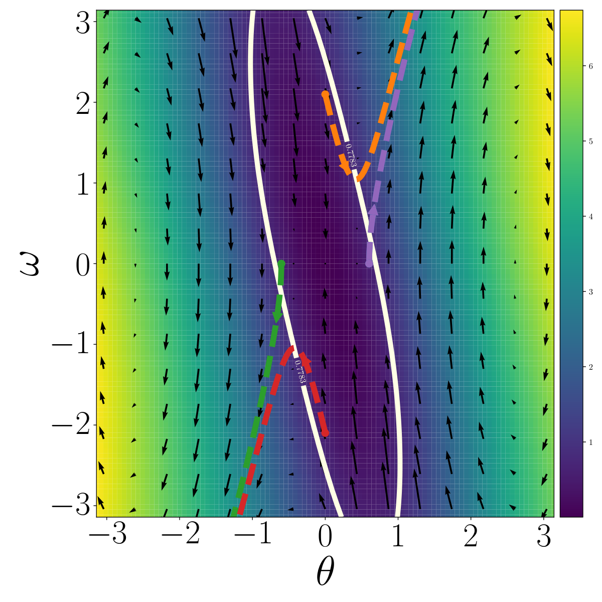
Figure 2 demonstrates an overestimation of the true RoA generated by the offline method called Neural Lyapunov Redesign (NLR, [5]), which does not consider uncertainties in the system dynamics. Figure 3 shows the percentages of RoA, forward invariant RoA, and estimated RoA over the entire state space. The enlargement of the true RoA and the estimated RoA based on our method are reflected in Fig. 4.

Next, we consider using an SMT solver to verify the CLF. Due to the SMT solver’s limit on the number of parameters, we consider a simpler setting for (IV-C). We reduce $f_{\theta_{1}}$, $\phi$, and $\psi$ to neural networks of three, two, and three layers, respectively. The nonlinear constraint (IV-C) is solved with $\zeta=0.3$ and a precision of $10^{-3}$, and no counter-example is found. This means that (13) is verified on the estimated RoA, which is around $34.6\%$.

Consider a third-order system of the strict feedback form:

The states are $(x_{1},x_{2},x_{3})$ and the state space is

Again, we assume that our initial knowledge of the system is not accurate: the true parameters are $e_{1}=1$, $e_{2}=1$, $e_{3}=1$, and $e_{4}=1$, while the nominal parameters are $e_{1}^{\prime}=0.9$, $e_{2}^{\prime}=0.8$, $e_{3}^{\prime}=0.9$, and $e_{4}^{\prime}=0.8$. Figure 5 shows the evolution of the percentages of RoA, forward invariant RoA, and estimated RoA along with a 3D visualization. We note that as our learning framework tries to stabilize more states, there can be transition periods where the size of the RoA drops, which might result from the sensitivity of the nonlinear controller to its weights. Figure 6 demonstrates ten randomly sampled trajectories starting from the boundary of the estimated RoA.

Finally, our method is tested on the cart-pole system:

The states are $(\theta,\omega,x,v)$, where $\omega=\dot{\theta}$ and $v=\dot{x}$. The state space is defined as

Note that $\theta=0$ corresponds to the upward position of the pole, and $\theta$ is positive in the counter-clockwise direction. The true parameters are $M=1$ $\mathrm{k}\mathrm{g}$, $m=0.3$ $\mathrm{k}\mathrm{g}$, $l=1$ $\mathrm{m}$, and $b_{c}=0$ $\mathrm{k}\mathrm{g}\,\mathrm{s}^{-1}$, while the nominal parameters are $M^{\prime}=0.8$ $\mathrm{k}\mathrm{g}$, $m^{\prime}=0.27$ $\mathrm{k}\mathrm{g}$, $l^{\prime}=0.8$ $\mathrm{m}$, and $b_{c}^{\prime}=0$ $\mathrm{k}\mathrm{g}\,\mathrm{s}^{-1}$. Figure 7 shows the evolution of the percentages of RoA, forward invariant RoA, and estimated RoA. Ten randomly sampled trajectories starting from the boundary of the estimated RoA are plotted in Fig. 8. The offline method NLR ([5]) generates an estimated forward invariant RoA ratio of 1.7% using the true parameters, which demonstrates the difficulty of this task. Finally, we test the robustness of the RoA estimation to sudden perturbations, where $b_{c}$ is increased to $9.1$ $\mathrm{k}\mathrm{g}\,\mathrm{s}^{-1}$. As seen in Fig. 9, our estimated RoA remains valid while the NLR estimated RoA no longer holds.

References

- [1] E. D. Sontag, “A ‘universal’construction of Artstein’s theorem on nonlinear stabilization,” Systems & Control Lett., vol. 13, no. 2, pp. 117–123, 1989.
- [2] S. M. Richards, F. Berkenkamp, and A. Krause, “The Lyapunov neural network: adaptive stability certification for safe learning of dynamical systems,” in Proc. Conf. on Robot Learning, (Zürich, Switzerland), Oct. 2018, pp. 466–476.
- [3] B. Dai, P. Krishnamurthy, A. Papanicolaou, and F. Khorrami, “State constrained stochastic optimal control using LSTMs,” in Proc. American Control Conf., (Virtual), May 2021, pp. 1294–1299.
- [4] B. Dai, P. Krishnamurthy, and F. Khorrami, “Learning a better control barrier function,” in Proc. IEEE Conf. on Decision and Control, (Cancun, Mexico), Dec. 2022, pp. 945–950.
- [5] A. Mehrjou, M. Ghavamzadeh, and B. Schölkopf, “Neural Lyapunov redesign,” in Proc. Annual Learning for Dynamics & Control Conf., (Virtual), June 2021, pp. 459–470.
- [6] S. Wei, X. Chen, X. Zhang, and C. Qi, “Towards safe and socially compliant map-less navigation by leveraging prior demonstrations,” in Proc. International Conf. on Intelligent Robotics and Applications, (Virtual), Nov 2020, pp. 133–145.
- [7] A. M. Lyapunov, “The general problem of the stability of motion,” International J. Control, vol. 55, no. 3, pp. 531–534, 1992.
- [8] Z. Artstein, “Stabilization with relaxed controls,” Nonlinear Analysis: Theory Methods & Appl., vol. 7, no. 11, pp. 1163–1173, 1983.
- [9] E. D. Sontag and Y. Wang, “On characterizations of input-to-state stability with respect to compact sets,” in Nonlinear Control Systems Design 1995. Pergamon, 1995, pp. 203–208.
- [10] P. Krishnamurthy and F. Khorrami, “On uniform solvability of parameter‐dependent Lyapunov inequalities and applications to various problems,” SIAM Journal on Control and Optimization, vol. 45, no. 4, pp. 1147–1164, 2006.
- [11] M. Krstić and P. V. Kokotović, “Control Lyapunov functions for adaptive nonlinear stabilization,” Systems & Control Lett., vol. 26, no. 1, pp. 17–23, 1995.
- [12] F. Berkenkamp, R. Moriconi, A. P. Schoellig, and A. Krause, “Safe learning of regions of attraction for uncertain, nonlinear systems with Gaussian processes,” in Proc. IEEE Conf. on Decision and Control, (Las Vegas, NV), Dec. 2016, pp. 4661–4666.
- [13] R. Sun, M. L. Greene, D. M. Le, Z. I. Bell, G. Chowdhary, and W. E. Dixon, “Lyapunov-based real-time and iterative adjustment of deep neural networks,” IEEE Control Syst. Lett., vol. 6, pp. 193–198, 2021.
- [14] A. J. Taylor, V. D. Dorobantu, M. Krishnamoorthy, H. M. Le, Y. Yue, and A. D. Ames, “A control Lyapunov perspective on episodic learning via projection to state stability,” in Proc. IEEE Conf. on Decision and Control, (Nice, France), Dec. 2019, pp. 1448–1455.
- [15] B. Tibken, “Estimation of the domain of attraction for polynomial systems via LMIs,” in Proc. IEEE Conf. on Decision and Control, (Sydney, Australia), Dec. 2000, pp. 3860–3864.
- [16] A. Papachristodoulou and S. Prajna, “On the construction of Lyapunov functions using the sum of squares decomposition,” in Proc. IEEE Conf. on Decision and Control, (Las Vegas, Nevada), Dec. 2002, pp. 3482–3487.
- [17] P. Giesl and S. Hafstein, “Review on computational methods for Lyapunov functions,” Discrete and Continuous Dynamical Systems - B, vol. 20, no. 8, pp. 2291–2331, 2015.
- [18] Y.-C. Chang, N. Roohi, and S. Gao, “Neural Lyapunov control,” in Proc. Conf. on Neural Information Processing Systems, (Vancouver, Canada), Dec. 2019.
- [19] T. Zhao, J. Wang, X. Lu, and Y. Du, “Neural Lyapunov control for power system transient stability: A deep learning-based approach,” IEEE Trans. on Power Systems, vol. 37, no. 2, pp. 955–966, 2021.
- [20] E. D. Sontag et al., “Smooth stabilization implies coprime factorization,” IEEE Trans. Autom. Control, vol. 34, no. 4, pp. 435–443, 1989.
- [21] S. Gao, J. Avigad, and E. M. Clarke, “-complete decision procedures for satisfiability over the reals,” in International Joint Conf. on Automated Reasoning, (Manchester, UK), June 2012, pp. 286–300.