Zero Curvature Condition for Quantum Criticality

Introduction. — Quantum phase transitions (QPTs) at zero temperature exhibit phenomena with no classical counterparts Vojta 2003; Sachdev 1999; Sachdev 2000; Zurek et al. 2005. While classical transitions are well described by the Landau-Ginzburg-Wilson (LGW) paradigm, quantum criticality poses deeper challenges due to the roles of entanglement and operator non-commutativity Vidal et al. 2003. In the LGW framework, transitions are driven by spontaneous symmetry breaking of local order parameters Landau 1937, a picture that fails to capture many QPTs. For example, topological phase transitions involve global invariants rather than local order parameters Wen 1989; Wen 1990; Wen and Wu 1993; Qi et al. 2008; Wen 2002; Wen 2017; Wen 2019. Another key case is deconfined quantum criticality, where continuous transitions emerge between competing orders, defying LGW expectations of first-order behavior or phase coexistence Senthil et al. 2004a; Senthil et al. 2004b; Shyta et al. 2022.

Several frameworks have been developed to characterize QPTs beyond the LGW paradigm. Information-geometric approaches equip the manifold of quantum states with a Riemannian structure Provost and Vallee 1980, using fidelity susceptibility and the quantum geometric tensor to detect criticality via singularities in ground-state overlaps Zanardi and Paunković 2006; Zanardi et al. 2007; Gu 2010. Entanglement-based methods describe critical states through scale-invariant tensor networks that efficiently capture long-range quantum correlations Vidal 2007. The onset of strong correlations near criticality also leads to a sharp increase in the sign problem Mondaini et al. 2022. Exceptional points in non-Hermitian systems provide another route, signaling criticality through spectral singularities Heiss 2012. Despite these advances, a general and physically transparent framework remains elusive, partly due to the diversity of microscopic mechanisms. A common structural feature, often implicit, is the non-commutativity of observables.

In this Letter, we introduce a geometric framework that places non-commutativity at the center. Rather than focusing on microscopic order, we study QPTs via the geometry of expectation values of competing non-commuting operators in the Hamiltonian. These define a quantum observable space (QOS), whose boundary encodes the interplay between operators. We show that this boundary is in one-to-one correspondence with ground states and serves as a geometric generalization of Heisenberg’s uncertainty principle. Quantum critical points emerge as zero-curvature points on the boundary, indicating maximal commutativity and potential integrability. This yields a representation-independent and experimentally accessible criterion for criticality, offering a complementary perspective beyond the LGW paradigm.

Convexity of Quantum Observable Space — We consider a quantum system with Hilbert space $\mathcal{H}$ and two semibounded Hermitian operators $H_{1},H_{2}\in\mathrm{Herm}(\mathcal{H})$, following the framework of Ref. Song 2023. These define a parametric Hamiltonian family

with real parameters $\lambda_{1},\lambda_{2}$ that govern the competition between generally non-commuting terms. The associated pure-state quantum observable space (QOS) is defined as

i.e., the set of all expectation value pairs over normalized pure states, which is also known as the joint numerical range Gustafson and Rao 1997; Bonsall and Duncan 1971. For finite-dimensional $\mathcal{H}$, $\mathcal{M}$ is a compact semialgebraic subset of $\mathbb{R}^{2}$, with a non-trivial boundary curve $\partial\mathcal{M}$, which plays a central role in our analysis (see Fig. 1a).

A key property of $\mathcal{M}$ is its convexity, as first shown by Brickman Brickman 1961 as an extension of the Hausdorff–Toeplitz theorem Toeplitz 1918; Hausdorff 1919. To see this, we observe that for any pair of states $|\psi_{1}\rangle$, $|\psi_{2}\rangle$, the interpolating superposition $|\psi(p)\rangle=\sqrt{p}\,|\psi_{1}\rangle+\sqrt{1-p}\,e^{i\theta}|\psi_{2}\rangle$ generates a continuous path connecting the corresponding points in $\mathcal{M}$, thereby tracing the entire segment between them for a suitable choice of $\theta$ and all $p\in[0,1]$ (see Appendix A). This implies that $\mathcal{M}$ is convex. An alternative argument based on Ehrenfest’s theorem and monotonicity also supports this conclusion Sørensen and Mølmer 2001.

This construction generalizes to any number $n$ of semibounded Hermitian operators $\{H_{1},\ldots,H_{n}\}$, defining the Hamiltonian family

Here, $\lambda_{i}$ are real if $H_{i}$ is bounded, and nonnegative if $H_{i}$ is only semibounded from below. The pure-state QOS generalizes to an $n$-dimensional set

For $n>2$, however, the set $\mathcal{M}$ is no longer guaranteed to be convex, with counterexamples such as the Bloch sphere. Nonetheless, convexity is restored when one extends to the mixed-state QOS,

where $\mathcal{D}=\{\rho\in\mathrm{Herm}(\mathcal{H})\colon\rho\geq 0\}$ is the space of density matrices. Since $\mathcal{D}$ is convex and the trace is linear, $\overline{\mathcal{M}}$ is convex by construction, as has been extensively studied in the theory of operator algebras Alfsen and Shultz 2012. Clearly, $\mathcal{M}\subseteq\overline{\mathcal{M}}$. Remarkably, these two sets actually coincide under mild conditions. If the observables $\{H_{i}\}$ are generic, i.e., their common eigenspaces form a set of measure zero, then $\mathcal{M}=\overline{\mathcal{M}}$ (see Appendix B). This requires the dimension of $\mathcal{H}$ to be no smaller than $\lceil n/2\rceil+1$, which always holds for $n=2$. In physically relevant settings, such as many-body systems in the thermodynamic limit or field-theoretic models with infinite-dimensional $\mathcal{H}$, the Hilbert space is sufficiently large that such a generic choice is almost surely satisfied. In such cases, the pure-state QOS is convex and coincides with its mixed-state counterpart. Throughout this work, we therefore identify $\mathcal{M}=\overline{\mathcal{M}}$, and thus their convexity, unless stated otherwise.

Geometric Uncertainty Principle — To analyze the structure of the quantum observable space $\mathcal{M}$, we consider the energy functional

with $\langle H_{i}\rangle\equiv\langle\psi|H_{i}|\psi\rangle$, and $|\psi\rangle\in\mathcal{H}$, $\|\psi\|=1$. The variational condition $\delta E[\psi]=0$ implies that stationary points correspond to eigenstates of the Hamiltonian (2), satisfying

The expectation values of eigenstates $|\psi_{e}(\bm{\lambda})\rangle$, for fixed $\bm{\lambda}=(\lambda_{1},\ldots,\lambda_{n})$, form a singular set

where the Jacobian of the map $|\psi\rangle\mapsto(\langle H_{1}\rangle,\ldots,\langle H_{n}\rangle)$ becomes rank-deficient Hartshorne 2013; Song 2023. Hence, the variational condition defines a critical variety, with $\bm{\lambda}$ as the local normal vector to $\mathcal{M}_{e}$.

For finite-dimensional $\mathcal{H}$, $\mathcal{M}_{e}$ forms an $(n-1)$-dimensional algebraic variety defined by a bivariate polynomial Song 2023. Of particular interest is the subset of ground states,

where $|\psi_{0}\rangle$ is the ground state. For semibounded operators, this corresponds to the lowest eigenstate. For bounded operators, either extremum may define the ground state depending on the sign of the Hamiltonian.

We find that the boundary of QOS coincides with this ground-state space (see Appendix C),

as a consequence of the supporting hyperplane theorem for convex sets Boyd and Vandenberghe 2004, together with the variational inequality

Equation (5) defines a geometric generalization of Heisenberg’s uncertainty principle. For example, the standard relation $\langle p^{2}\rangle\langle x^{2}\rangle\geq\hbar^{2}/4$ defines a QOS for the harmonic oscillator, with the saturation curve lying precisely on the boundary and realized by the ground state. Thus, the geometry of $\partial\mathcal{M}$ encodes fundamental quantum constraints on jointly observable quantities.

Zero Curvature Condition.— The convexity of $\mathcal{M}$ implies that the Gaussian curvature of its boundary $\partial\mathcal{M}$ is non-negative:

and more generally, the second fundamental form is positive semidefinite for $n>2$. This holds only for the ground-state manifold, reflecting its fundamental role in QPTs as distinct from excited-state behavior relevant to finite-temperature transitions.

In the thermodynamic limit, after rescaling observables by system size, $\partial\mathcal{M}$ may develop non-analyticities signaling QPTs. However, convexity restricts the types of singularities: for example, cusps may appear in excited-state geometry but not for ground states. The QPT appears as a singularity on $\partial\mathcal{M}$, where the curvature vanishes,

Two types of zero-curvature singularities may arise. Type I, illustrated in Fig. 2a, features a gap closing between two points $(\langle H_{1}\rangle^{*},\langle H_{2}\rangle^{*})$ and $(\langle H_{1}\rangle^{**},\langle H_{2}\rangle^{**})$, connected by a straight segment on $\partial\mathcal{M}$. This corresponds to a first-order transition with discontinuities $\Delta\langle H_{i}\rangle$ in order parameters and typically $\Delta E\neq 0$, though $\Delta E=0$ may occur under degeneracy. The common normal direction $\bm{\lambda}_{c}=(\lambda_{1c},\lambda_{2c})$ defines a single critical point. In contrast, Type II transitions, shown in Fig. 2b, occur at an isolated point with gap closing and continuous order parameters, but diverging derivatives, analogous to second-order transitions. In both cases, the zero-curvature condition $\kappa=0$ marks the criticality.

This geometry connects to the Ehrenfest classification. Setting $\lambda_{1}>0$, the coupling $g=\lambda_{2}/\lambda_{1}$ yields from Eq. (3) and the variational condition (4): $\langle H_{1}\rangle=E(g)-gE^{\prime}(g),\quad\langle H_{2}\rangle=E^{\prime}(g),$ via the Hellmann–Feynman theorem. The curvature becomes

showing that $\kappa=0$ implies a divergent second derivative. For non-degenerate ground states, perturbation theory gives $E^{\prime\prime}(g)=2\sum_{k>0}\frac{|\langle k|H_{2}|0\rangle|^{2}}{E_{0}-E_{k}}\leq 0,$ consistent with $\kappa\geq 0$, and vanishing as the gap $\Delta=E_{1}-E_{0}$ closes. In fact, $\kappa\sim\Delta$ near criticality. Our convexity result applies even in degenerate cases, extending beyond perturbative limits.

Type I and Type II transitions broadly correspond to first- and second-order phase transitions, respectively, but differ fundamentally from their classical counterparts. While classical transitions are typically driven by symmetry breaking, quantum transitions in our framework arise from the competition between non-commuting operators, imposing geometric constraints absent in classical theories. In particular, Type I transitions occur only at fixed normal directions $\bm{\lambda}_{c}$. As a result, they differ from classical first-order transitions, where coexistence spans a finite parameter region and involves mixed states, as described by Landau theory. In the quantum case, the ground state remains pure at zero temperature, and coexistence reflects degeneracy between distinct ground states. The system may interpolate between these extremal states with a fixed $(\bm{\lambda}_{c})$, but no extended coexistence region exists in the parameter space.

Furthermore, in systems involving more than two competing operators, the zero-curvature condition extends naturally to higher dimensions. In such cases, it defines critical geometries that delineate the phase boundaries of multidimensional phase diagrams.

Local Integrability.— To better understand the zero-curvature condition, we investigate the geometry of $\mathcal{M}$ in an integrable system. Let $H_{1},\ldots,H_{n}$ be a set of linearly independent, mutually commuting Hermitian operators acting on a finite-dimensional Hilbert space $\mathcal{H}$, with $\dim\mathcal{H}=n$. Without loss of generality, we may set $H_{n}=I$ and $\lambda_{n}=-E$, so that the Schrödinger equation takes the form $H|\psi\rangle=0$.

Since the operators commute, they can be simultaneously diagonalized as $H_{i}=\mathrm{diag}(\Lambda_{i1},\ldots,\Lambda_{in}),$ where $\Lambda_{ij}$ is the $j$-th eigenvalue of $H_{i}$. For any normalized state $|\psi\rangle=\sum_{j}\psi_{j}|j\rangle$, the expectation values are $\langle\psi|H_{i}|\psi\rangle=\sum_{j=1}^{n}\Lambda_{ij}|\psi_{j}|^{2}.$ The matrix $\Lambda=(\Lambda_{ij})$ is invertible due to the linear independence of the operators $\{H_{i}\}$. Defining its inverse $\tilde{\Lambda}=\Lambda^{-1}$, we obtain the relation $\sum_{j=1}^{n}\tilde{\Lambda}_{ij}\langle\psi|H_{j}|\psi\rangle=|\psi_{i}|^{2}\geq 0.$ Substituting $\langle\psi|H_{n}|\psi\rangle=\langle\psi|\psi\rangle=1$, we derive a set of $n$ linear inequalities:

where $\langle H_{j}\rangle=\langle\psi|H_{j}|\psi\rangle$. These inequalities define a simplex in $(n-1)$-dimensional space, and the boundary $\partial\mathcal{M}$ is given by the locus where equality holds in Eq. (8).

For any $n<\dim\mathcal{H}$, the geometry of $\mathcal{M}$ is obtained by projecting the $\dim\mathcal{H}$-dimensional simplex onto an $n$-dimensional subspace, resulting in a convex polytope. For example, when $H_{1}$ and $H_{2}$ commute in Eq. (1), the corresponding QOS is a polygon. The Gaussian curvature $\kappa$ of this polygon vanishes almost everywhere on the polygonal boundary, except at singular points where the boundary is non-differentiable. By contrast, for non-commuting operators, one typically observes a smooth, curved boundary. Therefore, the zero-curvature condition implies that the system near the critical point approximates an integrable limit, where the competing operators $H_{1}$ and $H_{2}$ are nearly commuting.

Examples.— We now apply our theory to several representative systems. One of the simplest examples of a QPT is the one-dimensional transverse field Ising model (TFIM) Pfeuty 1970, described by the Hamiltonian

where $X_{i}$ and $Z_{i}$ are Pauli matrices acting on site $i$, and $J$ and $h$ denote the spin interaction strength and the transverse field, respectively. In our setting, we identify $H_{1}=-\frac{1}{L}\sum_{i}Z_{i}Z_{i+1}$ and $H_{2}=-\frac{1}{L}\sum_{i}X_{i}$, where $L$ is the number of sites.

The TFIM follows the conventional LGW paradigm of symmetry breaking, with magnetization $m(g)\equiv-\langle H_{2}\rangle$ serving as the order parameter, where $g\equiv h/J$ is the dimensionless coupling. The model exhibits Kramers-Wannier duality, which interchanges $H_{1}$ with $H_{2}$ and $J$ with $h$, implying that $\langle H_{1}\rangle=-m(1/g)$ gives the magnetization of the dual system Pfeuty 1970. Figure 3a plots $\langle H_{1}\rangle$ versus $\langle H_{2}\rangle$, tracing the boundary of the quantum observable space $\mathcal{M}$. A quantum phase transition occurs at the critical point $g_{c}=1$ (marked by the red dot). The Gaussian curvature $\kappa$ can be computed using the exact magnetization in the thermodynamic limit Pfeuty 1970, yielding

where $K(x)$ and $E(x)$ are complete elliptic integrals of the first and second kinds. Figure 3b shows the curvature as a function of $g$, vanishing at the critical point in agreement with Eq. (7). Additionally, the curvature satisfies the self-duality relation $\kappa(g)=\kappa(1/g)$.

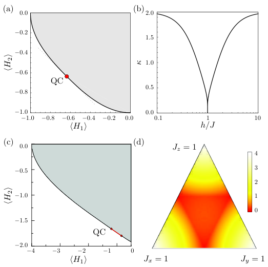
The TFIM is a special case of the quantum $q$-state Potts model with $q=2$. In 1D for $q>4$ or in 2D for $q>2$, the quantum Potts model undergoes a first-order phase transition Iglói and Sólyom 1983, which corresponds to a Type-I singularity in our classification. To verify this, Fig. 3c shows $\langle H_{1}\rangle$ versus $\langle H_{2}\rangle$ for the ground state, based on numerical data from Ref. Ding et al. 2017 (see Appendix E). The presence of a Type-I singularity is clearly visible.

While the two examples above fall within the Landau framework, we now turn to QPTs beyond the LGW paradigm. As a non-Landau example, we consider the Kitaev honeycomb model Kitaev 2006, defined on a hexagonal lattice with anisotropic bond-dependent interactions:

where $\langle ij\rangle_{\alpha}$ denotes nearest-neighbor pairs along the $\alpha=x,y,z$ directions. The model is exactly solvable and exhibits a topological QPT between gapped and gapless spin-liquid phases. The phase boundary is given by $|J_{\alpha}|=|J_{\beta}|+|J_{\gamma}|$ for all permutations of $\alpha\neq\beta\neq\gamma$ Feng et al. 2007; Chen and Nussinov 2008.

Here, the Hamiltonian involves three competing terms, and the QOS becomes a three-dimensional set with expectation values $\langle H_{\alpha}\rangle=-\sum_{\langle ij\rangle_{\alpha}}\langle\sigma_{i}^{\alpha}\sigma_{j}^{\alpha}\rangle$. The boundary $\partial\mathcal{M}$ forms a two-dimensional surface. We compute the Gaussian curvature analytically (see Appendix D),

where BZ is the Brillouin zone, and $\mathbf{u}(\mathbf{k})=|f|^{-3/2}\operatorname{Im}(f^{*}\mathbf{\Phi})$, with $f=\mathbf{J}\cdot\mathbf{\Phi}$ and $\mathbf{\Phi}_{i}=e^{i\mathbf{k}\cdot\mathbf{a}_{i}}$. The curvature is non-negative, consistent with convexity. Figure 3d shows $\kappa$ on the plane $J_{x}+J_{y}+J_{z}=1$, vanishing precisely on the analytically known phase boundary. This behavior can be understood analytically: at the phase boundary, two Dirac cones merge, leading to a quadratic band touching. The resulting dispersion causes the curvature integral to diverge, indicating vanishing curvature and thus confirming the zero-curvature condition for the topological transition.

Discussion.— We have introduced a geometric framework for QPTs that applies uniformly to both Landau and non-Landau types. In our approach, the competition between non-commuting operators defines a QOS, whose boundary encodes ground state information. Quantum criticality manifests as a singularity of this boundary, specifically at points of vanishing Gaussian curvature. We showed that both first- and second-order QPTs are associated with such zero-curvature points, albeit with distinct geometric signatures: discontinuous transitions correspond to flat segments, while continuous transitions are marked by smooth but non-analytic points where the curvature vanishes.

The emergence of zero curvature signals a local increase in commutativity among competing terms in the Hamiltonian and may reflect an underlying enhancement of symmetry. This observation resonates with results from conformal field theory, where many critical points admit integrable deformations under relevant perturbations Zamolodchikov 1989. Our findings suggest that quantum critical points may support effective integrable field theories in their vicinity, even when the underlying microscopic models are not integrable. Importantly, integrable systems near criticality often display strong entanglement and rich structure. Indeed, this geometric picture is consistent with the entropic formulation of the c-theorem Casini and Huerta 2007, which asserts that entanglement entropy is maximized at conformal fixed points and decreases monotonically along renormalization group flows away from criticality.

While our framework shares conceptual affinity with information-geometric approaches such as Provost–Vallee metric Provost and Vallee 1980 and the fidelity susceptibility Zanardi and Paunković 2006; Gu 2010, it differs operationally: our curvature is defined directly in the space of observable expectation values, making it experimentally accessible and free from coordinate ambiguity. Likewise, tensor-network approaches Vidal 2007 that capture scale-invariant entanglement at criticality may allow for a complementary geometric interpretation. In particular, the entanglement structure near criticality may be reflected in the shape and properties of the QOS boundary, offering a new lens on renormalization flow and universality.

This approach opens several promising directions for future work. One is the systematic classification of phase boundaries using algebro-geometric invariants of the QOS. In systems with more than two competing operators, the critical geometry may extend beyond isolated points or flat segments. While our analysis of the Kitaev honeycomb model demonstrates such a structure in three dimensions, a complete geometric characterization of criticality in higher-dimensional observable spaces remains an open challenge. Another intriguing direction is the potential connection to critical slowing down, where vanishing curvature may correspond to diverging timescales in the Kibble–Zurek mechanism. More broadly, our results suggest that quantum criticality can be understood as a geometric constraint arising from the non-commutativity of observables, offering a unified perspective on strongly correlated phases beyond the reach of traditional symmetry-based classifications.