On the origin of the non-detection of metastable Hei in the upper atmosphere of the hot Jupiter WASP-80b
Abstract
Aims. We aim to narrow down the origin of the non-detection of the metastable Hei triplet at 10830 Å obtained for the hot Jupiter WASP-80 b.
Methods. We measure the X-ray flux of WASP-80 from archival observations and use it as input to scaling relations accounting for the coronal [Fe/O] abundance ratio to infer the extreme-ultraviolet (EUV) flux in the 200–504 Å range, which controls the formation of metastable Hei. We run three dimensional (magneto) hydrodynamic simulations of the expanding planetary upper atmosphere interacting with the stellar wind to study the impact on the Hei absorption of the stellar high-energy emission, the He/H abundance ratio, the stellar wind, and the possible presence of a planetary magnetic field up to 1 G.
Results. For a low stellar EUV emission, which is favoured by the measured value, the Hei non-detection can be explained by a solar He/H abundance ratio in combination with a strong stellar wind, or by a sub-solar He/H abundance ratio, or by a combination of the two. For a high stellar EUV emission, the non-detection implies a sub-solar He/H abundance ratio. A planetary magnetic field is unlikely to be the cause of the non-detection.
Conclusions. The low EUV stellar flux, driven by the low [Fe/O] coronal abundance, is the likely primary cause of the Hei non-detection. High-quality EUV spectra of nearby stars are urgently needed to improve the accuracy of high-energy emission estimates, which would then enable one to employ the observations to constrain the planetary He/H abundance ratio and the stellar wind strength. This would greatly enhance the information that can be extracted from Hei atmospheric characterisation observations.
Key Words.
planets and satellites: atmospheres – planets and satellites: individual: WASP-80b1 Introduction
Seager & Sasselov 2000 and Oklopčić & Hirata 2018 showed that the metastable Hei (23S) triplet at 10830 Å in the near infrared can probe exoplanetary upper atmospheres in alternative to the ultraviolet (UV) band. Thus the Hei triplet can constrain atmospheric loss that plays a pivotal role in the evolution of exoplanets and in shaping their observed mass-radius distribution (Lopez & Fortney 2013; Jin et al. 2014; Jin & Mordasini 2018; Owen & Wu 2017; Kubyshkina et al. 2018; Modirrousta-Galian et al. 2020, e.g.).
The Hei atoms lying in the upper atmosphere can be excited to the metastable state either through photoionisation followed by recombination or through collisional excitation from the ground state (Andretta & Jones 1997). The former mechanism requires that the Hei atoms are irradiated by high-energy photons at wavelengths shorter than the Hei ionisation energy (504 Å or 24.6 eV), while the latter mechanism requires a high density of energetic electrons. Oklopčić & Hirata 2018 showed that in planetary atmospheres the photoionisation and recombination mechanism is significantly more efficient than the collisional excitation mechanism in producing metastable Hei. Instead, depopulation of the metastable state occurs through ionisation, radiative emission, and electron collisions, where the latter two mechanisms bring a Hei atom directly to the ground state or to the excited singlet state, which then decays to the ground state.
The relative efficiency of the mechanisms mentioned above, particularly those relying on photoionisation, strongly depend on the shape of the stellar spectral energy distribution (SED) irradiating a planet. Oklopčić 2019 showed that planets that are most likely to show metastable Hei absorption are those in close orbit around active stars with a low near-ultraviolet (NUV; 2600 Å) emission, that is active K-type stars. This is because an intense stellar X-ray and extreme ultraviolet (EUV; together XUV; 912 Å) emission enables ionisation of Hei atoms from the ground state, which can then recombine into the metastable state, while a low stellar NUV emission reduces the photoionisation of metastable Hei atoms.
Primary transit observations aiming at detecting metastable Hei absorption have been conducted for about 30 planets, with a positive detection in about ten cases (Spake et al. 2018; Nortmann et al. 2018; Salz et al. 2018; Allart et al. 2018; Alonso-Floriano et al. 2019; Ninan et al. 2020, e.g.). The observed systems span a wide range of stellar spectral types, from early A- to late M-type, and planetary properties, from small (presumably) rocky planets to gas giants. Some non-detections can be therefore explained by the star not having the appropriate SED (Nortmann et al. 2018, e.g. KELT-9 having a too low XUV flux and too high NUV flux;) and/or by the planet not having a large enough amount of He in its atmosphere (Krishnamurthy et al. 2021; Zhang et al. 2021, e.g. super-Earths such as Trappist-1b and 55 Cnc e;). Furthermore, the observations carried out so far have been obtained employing different instruments and techniques, namely ground-based high-resolution spectroscopy, ground- or space-based low-resolution spectrophotometry, and ground-based narrow-band photometry.
However, there have been also unexpected non-detections with the most striking being that of WASP-80b, which is an inflated hot Jupiter orbiting a K-type star. Fossati et al. 2022 reported the results of three high-quality transit observations of WASP-80b collected with the GIANO-B high-resolution spectrograph (Oliva et al. 2006) obtaining an upper limit on the Hei absorption of 0.7% (at the 2 level). This non-detection has been further confirmed by narrow band photometry observations (Vissapragada et al. 2022).
Fossati et al. 2022 also presented the results of three-dimensional (3D) hydrodynamic simulations of the upper atmosphere of WASP-80b and of its interaction with the stellar wind. They concluded that stellar wind pressure is unlikely to cause the non-detection and suggested instead that the atmosphere may have a low helium abundance relative to hydrogen (He/H) of at least ten times sub-solar. However, Vissapragada et al. 2022 suggested that confinement of the planetary atmosphere by a large-scale magnetic field might be responsible for the non-detection of metastable Hei.
As mentioned above, one of the key elements controlling the population and depopulation of the metastable 23S level is the stellar SED and in particular the part of the XUV emission primarily responsible for Hei photoionisation (i.e. 200–504 Å). This part of the stellar SED lies in the EUV band and it is observationally poorly constrained (France et al. 2019, see e.g.). Poppenhaeger 2022 derived scaling relations enabling one to infer the EUV emission in the 200–504 Å band on the basis of the stellar X-ray luminosity and [Fe/O] coronal abundance ratio, which could be measured from high enough quality X-ray spectra or inferred from stellar activity and age. Poppenhaeger 2022 concluded that for stars of similar X-ray luminosity, young and active stars with [Fe/O] 1, tend to have an EUV emission in the 200–504 Å band lower than that of old and inactive stars, with [Fe/O] 1.
In this work, we re-analyse the available X-ray spectra of WASP-80, as well as those of other planet-hosts, using the resulting X-ray flux to infer the EUV flux employing the scaling relations of Poppenhaeger 2022. We then use the obtained XUV flux as input to 3D hydrodynamic (HD) simulations to identify the possible origin of the non-detection of metastable Hei absorption. To test the suggestion of Vissapragada et al. 2022, we also employ 3D magneto hydrodynamic (MHD) modelling to estimate the impact of a planetary magnetic field on metastable Hei absorption. Finally, we place the results obtained for WASP-80b in the context of metastable Hei observations carried out for other systems.
This paper is organised as follows. Section 2 presents the results of a re-analysis of the XMM-Newton X-ray spectra of WASP-80. In Section 3, we describe the employed modelling scheme, while Section 4 presents the results of the (M)HD simulations. Section 5 shows a comparison of the results obtained for WASP-80b with those of past detections and non-detections present in the literature. Finally, Section 6 gathers the conclusions.
2 High energy emission of WASP-80
WASP-80 has been observed twice with XMM-Newton11 1 https://www.cosmos.esa.int/web/xmm-newton for a duration of 17 ks (obsid 0744940101, P.I. Salz) and 32 ks (obsid 0764100801, P.I. Wheatley). We retrieved the data from the XMM-Newton archive22 2 http://nxsa.esac.esa.int/nxsa-web/#search and reduced the constituent observation data files (ODFs) with the science analysis software (SAS) version 20.0 to obtain FITS tables of X-ray events calibrated in astrometry, arrival times, energies of events, and quality flags.
We selected the events in the 0.3–10 keV range, with PATTERN 12 and FLAG = 0 as prescribed by the SAS guide33 3 https://www.cosmos.esa.int/web/xmm-newton/how-to-use-sas. We checked the light curves of events at high energies (10 keV) to find periods of high background count rate during the observations. Observation 0744940101 was deemed free of high background intervals, while observation 0764100801 was affected by highly variable background, mostly for the pn detector. We retained only 5.3 ks of the 32 ks of the pn exposure at the end of this screening.

To accumulate the spectra of WASP-80, we extracted the events related to the target in circular regions of radius 30″ centered on the centroid of the X-ray source corresponding to WASP-80. The events used for background subtraction were extracted from a nearby circular region of radius 35″ (Figure 1). The spectra and the related response files were created with SAS. The spectra obtained for each observations from the MOS and pn detectors were combined together to have a summed spectrum with higher count statistics. The response matrices and the background spectra were also combined together with the SAS task epicspeccombine44 4 https://xmm-tools.cosmos.esa.int/external/sas/current/doc/epicspeccombine/index.html. The resulting so-called EPIC spectra were then grouped to have a minimum of 30 counts per bin. Summing up all spectra from MOS and pn, the spectra from the first and second exposures had 272 and 370 counts, respectively.
We then used the xspec55 5 https://www.cosmos.esa.int/web/xmm-newton/sas-thread-xspec software version 12.11.b to model the two EPIC spectra of both observations and infer NH absorption (i.e. hydrogen column density of the interstellar medium), mean temperatures (, ), emission measure, and flux () in the 0.2–10.0 keV band. The model was composed by the sum of two absorbed (tbabs model) thermal components (APEC). Hydrogen absorption and metal abundances were kept fixed. The resulting best fit parameters are listed in Table 1. The choice of this model was motivated by the fact that a simple one-temperature model with an absorbed APEC component gave ambiguous results. In fact, with this model the EPIC spectra could be described either by a low gas absorption of about 51020 cm-2 and a mean temperature around 0.7 keV or with a high gas absorption around 1022 cm-2 and a cooler temperature keV. As described below, there are solid motivations to discard this second solution at high .
| w2/w1 | |||||
|---|---|---|---|---|---|
| keV | keV | log(erg s-1 cm-2) | log(erg s-1) | ||
| Value | |||||
| C.I. | 13.85 to 13.69 | 27.6 – 27.8 |
The distance to the star is of about 49.7 pc (Gaia Collaboration et al. 2021) and at such a distance an interstellar medium hydrogen column density of order cm-2 is highly unlikely. To infer a more reliable NH value, we estimated an value of 0.161, to which we arrived by combining the observed color of 1.501 mag and the estimated intrinsic color mag expected for a main sequence star with an effective temperature of 4100 K such as WASP-8077 7 https://www.pas.rochester.edu/~emamajek/EEM_dwarf_UBVIJHK_colors_Teff.txt (Pecaut & Mamajek 2013). We remark that the value reported by Salz et al. 2015 appears to be too low for a star of spectral type K7 (i.e. K).
From , we inferred a value of A mag () and thus cm-2, which is of the same order of the value obtained from the best fit to the EPIC spectra ( cm-2). Fixing the hydrogen interstellar absorption to 51020 cm-2, the best fit gives an unabsorbed flux of erg s-1 cm-2 in the keV band and an X-ray luminosity of erg s-1.
This X-ray luminosity is comparable to those reported by Salz et al. 2015, King et al. 2018, and Fossati et al. 2022. We remark that the values given by Salz et al. 2015 and King et al. 2018 have been obtained considering a larger and less precise distance to the star compared to that measured by GAIA, which was not available at the time. Instead, Fossati et al. 2022 rescaled the X-ray luminosity given by King et al. 2018 accounting for the updated stellar distance, but did not consider that a shorter distance implies also a smaller value.
We estimated the EUV emission of WASP-80 in the 200–504 Å wavelength range starting from the measured X-ray flux value and considering the scaling relations of Poppenhaeger 2022, which we recall account for the [Fe/O] abundance in the stellar corona (i.e. high or low relative to solar). The X-ray spectrum of WASP-80 does not allow one to reliably measure the [Fe/O] coronal abundance, therefore we attempted to use the stellar age as proxy. In particular, it is possible to assign a [Fe/O] 1 coronal abundance to inactive stars older than 1 Gyr and with X-ray luminosity below erg s-1 and a [Fe/O] 1 coronal abundance to younger stars. This choice is driven by the low First Ionization Potential (FIP) effect observed in the Sun and in low activity stars (Laming 2021), where low FIP elements (such as Fe) appear to be over-abundant with respect to high FIP elements. At the same time, an inverse FIP effect is observed in high activity stars with Fe being under-abundant with respect to low FIP elements. Following Poppenhaeger 2022, this has a strong impact on the presence and strength of emission lines in the EUV band, and thus on the total EUV flux, such that at equal X-ray luminosity young and active stars have an EUV emission in the 200–504 Å range lower than that of old and inactive stars.
We estimated the age of WASP-80 using the isochrone placement algorithm presented in Bonfanti et al. 2015; Bonfanti et al. 2016. This routine interpolates the input parameters (in this case , [Fe/H], and ) within pre-computed grids of PARSEC88 8 PAdova and TRieste Stellar Evolutionary Code: http://stev.oapd.inaf.it/cgi-bin/cmd v1.2S (Marigo et al. 2017) isochrones and tracks to retrieve the best-fit age. For WASP-80, we obtained an age of 1.8 Gyr. Therefore, the stellar age is unconstrained, implying that it is not possible to clearly infer the coronal iron abundance, and thus the EUV emission. In the following, we consider that the star can have either a low/high [Fe/O] coronal abundance, and thus a low/high EUV emission (221 and 1520 erg cm-2 s-1 at the planetary orbit in the 200–504 Å wavelength range), and investigate the consequence in terms of formation and possible detection of Hei metastable absorption in the planetary atmosphere. However, we remark that the measured value of about 4.04 (Fossati et al. 2022) implies an age of 12 Myr (Mamajek & Hillenbrand 2008), which would therefore suggest that the lower EUV emission value might be preferable.
3 Modelling scheme
To simulate the upper atmosphere of WASP-80 b and its interaction with the stellar wind, we employ the 3D (M)HD code described by Shaikhislamov et al. 2018; Khodachenko et al. 2021b. It simulates self-consistently the expansion and escape of the planetary upper atmosphere, which is controlled by the stellar radiative heating and gravitational forces, and its interaction with the surrounding stellar wind, which is also simulated within the model. The extension enabling one to consider the planetary magnetic field strength is achieved adding to the set of hydrodynamic equations the magnetic field induction equation and the Ampere force in the momentum equations for the ionised species. We give here below a brief description of the modelling scheme.
The 3D hydrodynamic multi-fluid numerical model is run in a spherical coordinate system for which the polar axis is taken perpendicular to the orbital plane. For presenting the results we also use a Descart frame with the -axis directed along the planet–star line. The simulation reference frame is attached to the planet. Such geometry is suited well to simulate tidally locked planets with the stellar radiation impinging on the planet from just one direction, but we remark that the code enables one to simulate also planets with arbitrary rotation. The code solves numerically the continuity, momentum, and energy equations for separate components, which can be written in the following form (Shaikhislamov et al. 2016)
| (1) |
| (2) |
and
| (3) |
respectively. In the above equations, is the density of species , is time, is the velocity of species , is the mass of a particle of species , is the temperature of species , is the electron density, is the electron temperature, describes the gravitational interaction (see below), and is the heating term for the planetary atmosphere (see below). The terms , , , and are the photo-ionisation, charge-exchange, and collisional terms listed in Table 1 of Shaikhislamov et al. 2016.
The main processes responsible for the transformation between neutral and ionised particles are photoionisation, electron impact ionisation, and dielectronic recombination, which are included in the term in Equation (1) and are applied to all species. Photoionisation also results in heating of the planetary gas through impacts with the produced photoelectrons. The corresponding heating term in Equation (3) (Shaikhislamov et al. 2014; Shaikhislamov et al. 2016; Khodachenko et al. 2015, see) comprises terms derived by integrating the stellar XUV spectrum in the 10–912 Å wavelength range (e.g. Equation (4) of Khodachenko et al. 2015 and Equation (5) of Shaikhislamov et al. 2016). The model assumes that the energy released in the form of photoelectrons is rapidly and equally redistributed among all nearby particles with efficiency = 0.5 1. This is a commonly used assumption, which we adopted on the basis of qualitative analyses (Shaikhislamov et al. 2014). The heating term, which includes also energy loss due to excitation and ionisation of hydrogen atoms, in a simplified form can be written as
| (4) |
where is the frequency of the stellar irradiation, is the ionisation energy, is the cross-section to the stellar XUV flux , is the excitation energy, and and are respectively the ionisation and excitation cross sections averaged over a Maxwellian distribution of electrons.
The model further accounts for resonant charge-exchange collisions (), which at low energies has a cross-section of = 610-15 cm-2 that is an order of magnitude larger than the elastic collision cross-section. Experimental data on the differential cross-sections can be found, for example, in Lindsay & Stebbings 2005. Since planetary atoms and protons have different thermal pressure profiles and protons feel electron pressure while atoms do not, when they pass close to each other the charge-exchange between them leads to velocity () and temperature () exchanges. We describe this process with the collision rate , where the upper index indicates the value being exchanged. For example, in the momentum equation for planetary protons there is the term = , where the interaction velocity depends in general on the thermal and relative velocities of the interacting fluids, in this specific case protons and neutral atoms of the planetary wind. More accurate expressions for the charge-exchange terms present in the continuity, momentum, and energy equations, obtained by averaging the collision operator over the Maxwell distribution (Meier & Shumlak 2012, e.g.), differ from those used in our model by less than a factor of a few, which is negligible for the purposes of the simulations.
In the model, we considered the following cross-sections: = 6.310-18(/)3 cm2 as the wavelength dependent XUV ionisation cross-section, = 4.010-16T-1 cm2 as the electron impact ionisation cross-section, = 6.710 cm2 as the cross-section for recombination with electrons, and = 3 cm2 and = 710 cm2 as the hydrogen excitation and de-excitation cross-sections, respectively, where the temperature is scaled in units of the model’s characteristic temperature (i.e. K), except in the exponents for the expressions of and , where the temperature is given in erg.
For the typical parameters of planetary plasmaspheres, Coulomb collisions with protons effectively couple the minor species’ ions. For example, at K and cm-3 the collisional equalisation time (Braginskii 1965) for temperature and momentum
| (5) |
is about 2 s for protons and about 8 s for He. This is several orders of magnitude smaller than the typical gas-dynamic time scale of the problem treated here, which is of the order of 104 s.
The strong coupling of charged particles in the planetary wind on the considered typical spatial scale of the problem (i.e. about Rrmp; 1010 cm) is further justified by the presence of a chaotic and sporadic magnetic field in the planetary wind, which affects the relative motion of the ions so that they become coupled through the Lorentz force and exchange their momentum on the time scale of the Larmor period. For the same reason, charged particles can be treated as strongly coupled ones in the hot and rarefied stellar wind as well, even in spite of the fact that Coulomb collisions are negligible there. Therefore, there is no need to calculate the dynamics of every charged component of the plasma fluid species, and we assume all of them to have the same temperature and velocity. Instead, the temperature and velocity of each neutral component is calculated individually by solving the corresponding energy and momentum equations. The neutral hydrogen atoms are more or less coupled to the main flow also by elastic collisions. With a typical cross-section of 10-16 cm2, the mean-free path at a density of 106 cm-3 is comparable to the planetary radius. Besides elastic collisions, charge exchange ensures more efficient coupling between hydrogen atoms and protons (Shaikhislamov et al. 2016; Khodachenko et al. 2017). Furthermore, the simulation is simplified by assuming that all charged particles have the same velocity, while each neutral fluid has its own particular velocity, including Hei and Hei (23s).
The model further accounts for molecular hydrogen and the corresponding ions (Khodachenko et al. 2015; Shaikhislamov et al. 2018, H, H; see), which allows more accurate treatment of the inner regions of the planetary thermosphere and cooling by the efficient infrared emitter H. The model enables also the inclusion of minor species, which are described as separate fluids by the corresponding momentum and continuity equations. The population of different ionisation states for each element is calculated assuming the specific photoionisation (Verner & Ferland 1996) and recombination rates (Le Teuff et al. 2000; Nahar & Pradhan 1997). We remark that we do not consider chemical reactions among the different minor species, while the list of modelled hydrogen reactions can be found in Khodachenko et al. 2015, and it is comparable to that used in other aeronomy models (García Muñoz 2007; Koskinen et al. 2007, e.g.).
To account for the geometry of the problem, we employ a gravitational potential that accounts for rotational effects of the form
| (6) |
where the subscript indicates the star.
The numerical scheme is explicit and uses an up-wind donor cell method for flux calculations. To achieve second order spatial accuracy for differentials, we consider two grids shifted by half a step along each dimension. One grid is reserved for densities, temperatures, and gravity potential, and the other for velocities. For second order temporal accuracy at each time step, the code calculates at first (,) values using the velocity field and then recomputes using the new (,) values. The numerical scheme fully conserves flux and total mass, and conserves the Bernoulli constant along the characteristics. For energy, a simple non-conservative equation is used. The energy conservation is checked by global integration and is used to evaluate the accuracy of the simulation. Usually, the energy is balanced within 25%. We do not use any particular method to capture the shock between planetary and stellar wind. For the problems under consideration, the accurate position of the shock and high front resolution are not crucial.
The spatial spherical grid uses uniform step for azimuth angle (in this particular study we employ 96 points along a circumference; i.e. = 0.065). The radial grid is exponential with steps varying linearly with radius as = , where is the planetocentric radial distance. At the planetary surface is as small as /200. For , we employ a value equal to . Therefore, in the shock region of about 20 the resolution is about . For the polar angle, the grid is quadratic, , with the smallest step located at the equatorial plane. Usually, at the equator and along the polar axis. We note that the exponential radial spacing in the spherical coordinate system allows one to keep the same resolution in all three dimensions, if the azimuthal and latitudinal steps are chosen so that . The influence of spatial resolution has been checked by doubling the number of grid points for each dimension obtaining comparable results.
Each simulation is started from an initial static atmosphere and proceeds in the case of WASP-80b for about 500 dimensionless times (corresponding to about 14 orbits) until the overall planetary mass-loss rate reaches 95% of its asymptotic level, which is judged to be sufficient to assume that the simulation has reached the steady state.
To compute the column densities along stellar rays, we use integration from the star to each cell in the planetary spherical frame, using along the path the density values interpolated from nearby pixels. The calculated column density is used to determine the attenuation of the stellar XUV flux in each spectral bin of 0.1 nm. To save numerical time, the radiation transfer is calculated usually each forth step of fluid dynamics and chemistry. We assume optically thin approximation for the photons generated by proton recombination to the ground state, and thus the total recombination coefficients are used.
The chemical reactions are calculated by direct conversion of the matrix at each time step and at each pixel. This is not efficient numerically, but eliminates convergence problems due to the widely different reaction rates .
Because of the large scale of the considered system, in most of the area surrounding the planet the dynamics of the magnetic field is assumed to be dissipation-less, which in the numerical model is achieved by taking a sufficiently high, though finite, electric conductivity corresponding to a magnetic Reynolds number of about 105. This value was found empirically to exceed the numerical diffusion in the magnetic field induction equation. The planetary magnetic dipole moment is directed perpendicularly to the equatorial plane, which is considered to be coplanar to the ecliptic plane.
In the case of the MHD simulations, we calculate the magnetic field induction equation assuming that the divergence of the magnetic field is zero. At the inner boundary of the computation domain (i.e. at the optical radius of the planet = ), we fix the flux of the magnetic field by fixing the radial component of the magnetic dipole field (i.e. = constant). Instead, the perturbations of the azimuthal (i.e. toroidal; ) and poloidal () components of the field obey an open boundary condition that is , where the symbol indicates the perturbation (Khodachenko et al. 2021b). The code has already been used to interpret the observations of metastable Hei absorption for GJ3470 b (Shaikhislamov et al. 2021), WASP-107 b (Khodachenko et al. 2021a), and HD189733 b Rumenskikh et al. 2022, as well as for HD209458 b in case it hosts a magnetic field (Khodachenko et al. 2021b).
4 Results
4.1 Non-magnetised planet


| He/H | XUV - EUV | XUV - EUV | Peak | FWHM | ||
| at 1 AU | at planet | absorption | absorption | |||
| [erg cm-2 s-1] | [erg cm-2 s-1] | [1012 g s-1] | [1010 g s-1] | [%] | [km s-1] | |
| 0.01 | 0.125 - 0.051 | 105.6 - 43.3 | 0.1 | 0.02 | 0.10 | 10 |
| 0.01 | 0.25 - 0.10 | 211.3 - 86.6 | 0.1 | 0.06 | 0.24 | 11 |
| 0.01 | 0.31 - 0.13 | 262.0 - 107.4 | 0.1 | 0.08 | 0.29 | 11 |
| 0.01 | 0.5 - 0.2 | 422.5 - 173.2 | 0.1 | 0.15 | 0.48 | 11 |
| 0.01 | 1.8 - 0.7 | 1521.1 - 623.6 | 0.1 | 0.68 | 0.79 | 13 |
| 0.01 | 4.4 - 1.8 | 3718.2 - 1524.5 | 0.1 | 1.70 | 1.66 | 20 |
| 0.01 | 7.5 - 3.1 | 6337.9 - 2598.5 | 0.1 | 2.80 | 1.81 | 20 |
| 0.03 | 0.31 - 0.13 | 262.0 - 107.4 | 0.1 | 0.07 | 0.72 | 11 |
| 0.03 | 1.0 - 0.4 | 845.1 - 712.9 | 0.1 | 0.29 | 1.83 | 12 |
| 0.03 | 4.4 - 1.8 | 3718.2 - 1524.5 | 0.1 | 1.58 | 3.23 | 19 |
| 0.1 | 0.125 - 0.051 | 105.6 - 43.3 | 0.1 | 0.01 | 0.44 | 11 |
| 0.1 | 0.5 - 0.2 | 422.5 - 173.2 | 0.1 | 0.05 | 1.81 | 12 |
| 0.1 | 1.8 - 0.7 | 1521.1 - 623.6 | 0.1 | 0.24 | 4.09 | 13 |
| 0.1 | 7.5 - 3.1 | 6337.9 - 2598.5 | 0.1 | 1.72 | 7.79 | 16 |
| 0.1 | 4.4 - 1.8 | 3718.2 - 1524.5 | 20 | 1.47 | 3.23 | 13 |
| 0.1 | 0.6 - 0.24 | 507.0 - 202.8 | 20 | 0.37 | 0.95 | 12 |


For all simulations, we considered the near-ultraviolet and near-infrared stellar emission given by Fossati et al. 2022 and a planetary orbital separation of 0.0344 (Triaud et al. 2015). We ran simulations for a range of stellar EUV (i.e. 200–504 Å) and XUV (10–912 Å) emission flux values that encompass those derived in Section 2, as well as three He/H abundance values of 0.01, 0.03, and 0.1 (by number), where the latter is the solar He/H abundance ratio. At the lower atmospheric boundary, which we locate at a pressure of 0.05 bar, we considered a planetary atmospheric temperature of 1000 K. To model the stellar wind, we considered the same parameters taken by Fossati et al. 2022 that is a velocity of 200 km s-1, a temperature of 0.7 MK, and a density of 103 cm-3 at the position of the planet, corresponding to an integral stellar mass-loss rate of 1011 g s-1. The main difference with the work of Fossati et al. 2022 lies in the significantly smaller stellar XUV emission: they employed a stellar XUV emission at 1 AU of 7.5 erg cm-2 s-1 that is the largest value considered in this work. This is due to the fact that the scaling relations of Poppenhaeger 2022 lead to smaller EUV flux values compared to those of King et al. 2018 that were used by Fossati et al. 2022. Given the measured X-ray luminosity, the stellar wind strength expected for WASP-80 is 21013 g s-1 (Vidotto 2021). Therefore, we have further performed two additional runs considering a He/H abundance ratio of 0.1, a stellar wind mass-loss rate of 21013 g s-1, and the two XUV flux values (221 and 1520 erg cm-2 s-1) computed from the scaling relations of Poppenhaeger 2022 either assuming a low or high [Fe/O] coronal abundance.
The detailed results of the hydrodynamic simulations, such as the density distribution and temperature profile, resemble those presented by Fossati et al. 2022. As an example, Figure 2 shows the proton density distribution in the planetary orbital plane obtained from the run computed considering a He/H abundance ratio of 0.01 and an EUV stellar flux at 1 AU of 0.7 erg cm-2 s-1. The map shows the presence of two gas streams departing from the planet, towards (in front) and away (behind) from the planet. The planetary material after initial spherical expansion is forced to move close to the planetary orbit due to momentum conservation. The stream ahead of the planets is composed by escaped gas that feels the stellar gravitational pull and stops as a result of the interaction with the stellar wind. The stream behind the planet, also composed by planetary escaped gas, is a typical characteristic of close-in giant planets with an escaping atmosphere (Bourrier et al. 2016; Esquivel et al. 2019; Shaikhislamov et al. 2018; McCann et al. 2019; Debrecht et al. 2020; Carolan et al. 2021; MacLeod & Oklopčić 2022, e.g.). Figure 3 shows as an example the absorption profiles obtained from time averaging (Dos Santos et al. 2022, see) in the 0.1 to 0.1 planetary orbital phase range, which is the same range taken into account to extract the observed transmission spectrum from the data (Fossati et al. 2022, see Figure 1 of ), and considering a He/H abundance ratio of 0.01. We note that averaging reduces the peak absorption by less that 5%. Interestingly, in the case WASP-80b, we find that the cometary tail forming behind the planet does not produce significant metastable Hei absorption, in contrast to what found by MacLeod & Oklopčić 2022 for other systems.
Given the similarities of the detailed results with those of the simulations presented by Fossati et al. 2022, we focus here on the obtained planetary metastable Hei absorption and mass-loss rate values. All results derived from the HD simulations are summarised in Table 9 and displayed in Figure 4. The full width at half maximum (FWHM) listed in Table 9 is a measure of the velocity of the Hei metastable atoms along the line of sight, and thus it is directly linked to the structure and asymmetry of the absorbing atmosphere. This is key information that can be accurately extracted and compared with observations exclusively employing 3D simulations such as those adopted in this work.
We find that both metastable Hei absorption and mass-loss rate increase roughly linearly with increasing high-energy stellar emission and the Hei absorption is strongly dependent on the He/H abundance ratio. Furthermore, with increasing He/H abundance ratio, the mean molecular weight increases, which leads to a decrease of the pressure scale height, and thus of the atmospheric extension and consequently of the mass-loss rate.
Considering a stellar EUV emission at the planetary orbit of 1520 erg cm-2 s-1 (i.e. the higher of the two obtained from the scaling relations; see Section 2), we find that the non-detection of metastable Hei absorption implies a He/H abundance ratio smaller than ten times sub-solar. Instead, with the lower EUV stellar emission value, which is favoured by the measured value, we obtain that metastable Hei absorption would have been undetectable for a solar He/H abundance ratio in combination with a stellar wind stronger than that expected on the basis of the measured X-ray luminosity, or for a slightly sub-solar He/H abundance ratio, or for a combination of the two. For a solar He/H abundance ratio and the foreseen stellar wind strength, the metastable Hei detectability level of the observations corresponds to a stellar XUV flux value that is about 1.5 times lower than the smaller one obtained following the scaling relations of Poppenhaeger 2022. As expected, an increase in the stellar wind mass-loss rate leads to a decrease in the metastable Hei absorption signal (Vidotto & Cleary 2020; Fossati et al. 2022), however it does not appear to be enough to explain the non-detection without the need of a sub-solar He/H abundance ratio or of a stellar wind stronger than that foreseen on the basis of the measured X-ray luminosity or of both.
4.2 Magnetised planet
To test the suggestion of Vissapragada et al. 2022, we further modelled the WASP-80 system considering a magnetised planet with a field strength of up to 1 G (i.e. comparable to that of Jupiter). To properly study the impact of a planetary magnetic field on the absorption of metastable Hei, we employed a stellar spectral energy distribution with an XUV emission strong enough to ensure the production of enough metastable Hei to lead to significant absorption. Therefore, for the MHD simulations, we considered the stellar SED used by Fossati et al. 2022, namely an XUV and EUV flux equal to the strongest one considered for the HD simulations. To isolate the effect of the planetary magnetic field, we take a sufficiently low He/H abundance ratio of 0.01, so that it does not influence the formation of the planetary wind and its interaction with the stellar wind, yet providing sufficient metastable Hei absorption. Finally, we employed a stellar wind with a mass-loss rate of 1011 g s-1.
We run simulations for a planet with a very low magnetic field of 0.01 G, which leads to results equivalent to those of a non-magnetised planet, and two cases with a relatively strong magnetic field of 0.5 and 1.0 G. For the strongest planetary magnetic field, we also simulated the case of a moderately strong stellar wind, that is 20 times higher density, in which the magnetised planet generates a typical magnetosphere. The main input parameters and resulting planetary mass-loss rate and metastable Hei absorption are summarised in Table 10.
| N | AHeI | ||||
|---|---|---|---|---|---|
| [G] | [] | [1011 g s-1] | [1010 g s-1] | [%] | |
| 1 | 0.01 | 0.002 | 1 | 2.9 | 1.24 |
| 2 | 0.5 | 0.1 | 1 | 1.5 | 0.74 |
| 3 | 1.0 | 0.2 | 1 | 0.9 | 0.57 |
| 4 | 1.0 | 0.2 | 20 | 0.9 | 0.95 |
Figures 5 and 6 show the electric currents generated by a magnetised planet. As obtained from previous 2D and 3D simulations (Khodachenko et al. 2015; Khodachenko et al. 2021b), as well as earlier semi-analytical considerations (Khodachenko et al. 2012), the outflowing planetary wind gas stretches and opens the magnetic dipolar field lines, forming an equatorial current layer, that is the so called magnetodisk.


The magnetodisk is thin and surrounds the planet in the equatorial plane, but not uniformly, because of the planetary flow clock-wise rotation due to the Coriolis force. Also, there is a cavity close to the planet, the so called dead zone, where planetary material is stagnant. The generated magnetospheric system of currents is characterised by a region around the planet dominated by the dipolar magnetic field, a current sheet at the front of the magnetosphere (i.e. the magnetopause), a current sheet at high latitudes, and a current sheet forming a tail behind the planet. The strong stellar wind generates a clear bow shock around the planet, which appears to have a structure similar to that of the magnetised solar system planets (Figure 6).
Figure 7 shows the proton density distribution obtained from the model run N3 (see Table 10). A comparison between Figures 2 and 7 indicates that a strong planetary magnetic field truncates the tail behind the planet, which is predicted to be a prominent feature for non-magnetised planets (MacLeod & Oklopčić 2022). This suggests that the presence of a cometary tail could indicate the absence of a strong planetary magnetic field. The field also shortens the gas stream lying ahead of the planet further bending it towards the star.

The profiles shown in Figure 8 give further details on the structure of the planetary outflow. In the case of the weaker planetary magnetic field (model run N1), the expanding planetary atmosphere is stopped relatively far from the planet, with the acceleration being driven by absorption of the stellar XUV emission and subsequent atmospheric heating. In this case, the atmosphere becomes supersonic at a distance of about 4.5 planetary radii. For a planetary magnetic field strength of 0.5 G (model run N2), the planetary flow is strongly decelerated by the force of the magnetic tension (except at the open field lines region; see Khodachenko et al. 2015; Khodachenko et al. 2021b, for more details) and the velocity is smaller by a factor of two at distances shorter than five planetary radii compared to the case of a weakly magnetised planet. In the case of the strongest planetary magnetic field and stellar wind (model run N4), there is the formation of a magnetopause and bow shock. The position of the magnetopause, analytically computed as
| (7) |
is close to the one obtained by the simulation (about 5.5 ). Within the magnetopause, the planetary wind velocity is about an order of magnitude smaller than that obtained for the case of the weakly magnetised planet. Indeed, the magnetic pressure prevails over the thermal pressure up to 3 , becoming instead comparable close to the magnetopause.


Figure 9 shows the synthetic metastable Hei absorption profiles in comparison to the observations of Fossati et al. 2022. Despite the planetary magnetic field has significantly modified the structure of the upper atmosphere, compared to the almost non-magnetised case, the Hei absorption decreases by less than a factor of two. However, with a stronger stellar wind the absorption increases, reaching almost the same level as that obtained for the almost non-magnetised planet. This occurs, because with the stronger stellar wind the magnetosphere compresses, increasing the overall density of the absorbing material around the planet.

These results indicate that a planetary magnetic field is unlikely to be the source of the non-detection of metastable Hei absorption in the atmosphere of WASP-80b. This is primarily, because most of the absorption (i.e. the peak absorption) takes place close to the planet for which the influence of the magnetic field is not particularly strong, while the differences in the absorption maps shown in Figure 10 affect mostly the line wings, which form farther away from the planet and thus do depend on the planetary magnetic field strength.

In regard of the polar regions, the simulations indicate that the planetary magnetic field reduces the outflow velocity resulting to a decreased density over the poles (see Trammell et al. 2014; Khodachenko et al. 2015; Carolan et al. 2021, for a detailed discussion on the effect of a planetary magnetic field on the outflow velocity at the polar regions). However, because of the lower velocity, the planetary outflowing gas is more strongly photoionised, resulting in larger electron densities, which lead to a larger population of metastable Hei atoms produced through recombination of Heii. Furthermore, by reducing the outflow velocity, the planetary magnetic field reduces the width of the absorption of the Hei (23S) feature from about 19 km s-1 at = 0.01 G to about 12 km s-1 at = 1.0 G. Indeed, Figure 8 shows that close to the planet the outflow velocity decreases with increasing magnetic field, but the outflow velocity is generally small and thus the reduction of the velocity does not significantly impact the absorption strength. Finally, Figure 9 shows that with increasing planetary magnetic field from 0.5 to 1.0 G, the population of high velocity (i.e. from about 30 to 10 km s-1) metastable Hei atoms decreases significantly, in agreement with the previous analysis.
5 Discussion
We place our results in the context of observations published for other systems. We collected the physical properties of the systems for which either measurements or non-detections of metastable Hei absorption have been published (Table 4). For consistency, we re-analysed archival X-ray data for some of the systems and applied the scaling relations of Poppenhaeger 2022 to all of them.
5.1 High-energy emission
We gathered the system parameters from the literature, giving priority to more recent and/or homogeneous sources. For the systems considered by Poppenhaeger 2022, we took their reported X-ray luminosity, while for the other systems we derived the X-ray luminosity from archival observations (Table 13). To this end, we searched for X-ray observations in the XMM-Newton and Chandra archives. All necessary data, except for WASP-52, were found in pointed XMM-Newton observations or in the slew survey. WASP-52 was observed with Chandra for about 10 ks. For the targets in pointed and publicly available XMM-Newton observations (WASP-80, 55 Cnc, HAT-P-32, and Trappist-1), we reduced the datasets with SAS version 20.0, extracted the spectra, and performed the best fit analysis using XSPEC version 12.11.
Details about the X-ray data of WASP-80 are given in Section 2. In general, we used a combination of 1 or 2 APEC thermal models absorbed by a global equivalent H column (tbabs model), where the free parameters were the temperature (), the normalisation of each component, the NH equivalent column gas absorption, and the global abundances (). However, for WASP-80 we kept fixed NH and , as motivated in Section 2. For Trappist-1, observed in six different XMM-Newton visits, we extracted separately the pn and MOS spectra, combining them with SAS to obtain an average spectrum with the highest count statistics to then perform a simultaneous fit. For WASP-52 we accumulated the count rate in a region 5″ wide and used PIMMS1111
11
https://heasarc.gsfc.nasa.gov/docs/software
/tools/pimms.html to estimate its flux, using a single APEC model with = 0.1 keV and solar abundance. For the undetected stars in XMM-Newton, we computed the flux starting from the pn count rate in the 0.2–12 keV band, using an optically thin thermal APEC model at 0.1 keV with solar abundances and cm-2 to estimate the unabsorbed flux in the 0.2–10 keV band. For V 1298 Tau, we adopted the results of Maggio et al. 2022, who employed the same data analysis technique we used for the other stars.
As for WASP-80, we estimated the stellar EUV emission in the 200–504 Å wavelength range starting from the X-ray measurements and considering the scaling relations of Poppenhaeger 2022. The [Fe/O] abundance of the stellar corona has been measured from the available X-ray spectra just for a few stars in our sample. For the systems in common, we took the [Fe/O] abundance value given by Poppenhaeger 2022, while for the other systems we estimated the [Fe/O] abundance based on the activity and age of the host stars (Table 14). For each star in the sample, we estimated the age by using the isochrone placement algorithm briefly described in Section 2 (Bonfanti et al. 2015; Bonfanti et al. 2016).
We derived the isochronal age for each star in the sample, except for Trappist-1 and GJ1214 that are extremely low-mass stars. For stars of this type, the stellar parameters are almost constant over time. For example, PARSEC models predict maximum variations of 0.2% on a time scale comparable to the age of the universe. Therefore, it is not possible to infer the age from evolutionary models, however other indicators may help distinguish between young and old stars.
Filippazzo et al. 2015 studied a sample of ultra-cool dwarfs, also containing Trappist-1. They evaluated the ages according to youth indicators, such as the membership to nearby young moving groups (Gagné et al. 2015, see e.g.) or the - gravity suffix that can be inferred from spectra (Kirkpatrick 2005; Cruz et al. 2009). In the case of Trappist-1, no clear youth signatures were detected, yielding to a lower age limit of 0.5 Gyr. For GJ1214, Berta et al. 2011 did not detect any kind of activity-induced chromospheric emission in either H or the Nai D lines. They estimated the stellar rotation period being a multiple of 53 d, which suggests a low magnetic activity. By applying the relation from West et al. 2008 between magnetic activity and kinematic age, they inferred an age greater than 3 Gyr and confirmed this by computing the stellar motion in the velocity space finding km s-1, which is consistent with membership to the Galactic old disk.
5.2 Comparison with WASP-80b
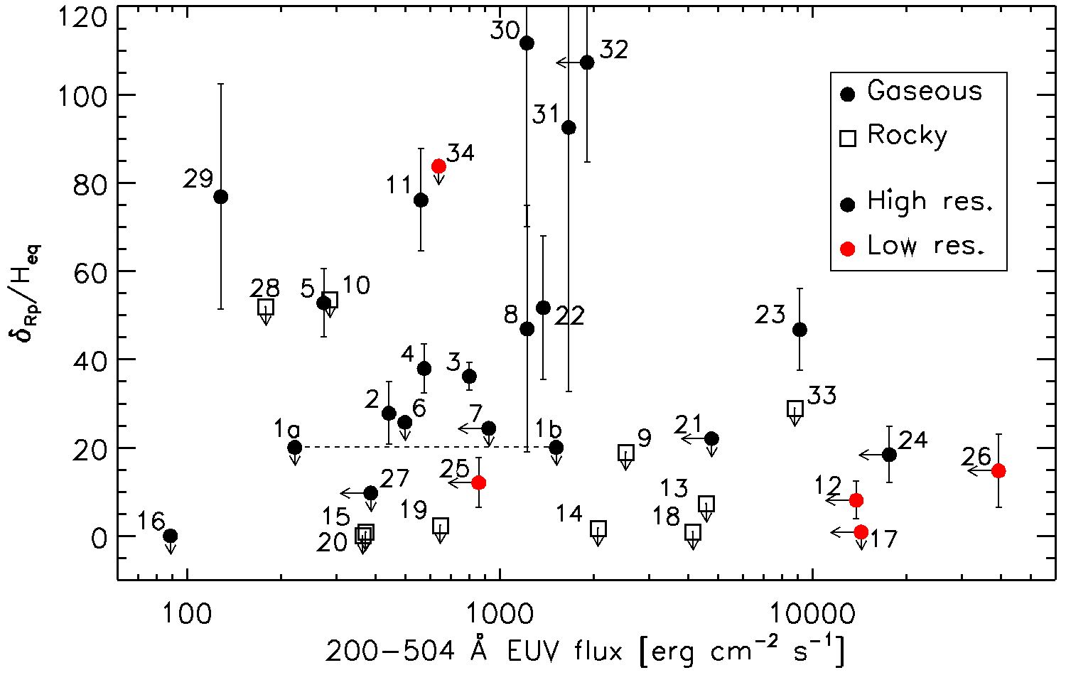
Figure 11 shows the size of the measured Hei absorption signal or upper limit (), normalised to the atmospheric scale height (), as a function of incident stellar EUV flux in the 200–504 Å wavelength range (Poppenhaeger 2022). For each system, we estimated using the data listed in Table 4 and following Fossati et al. 2022. The upper limits on the Hei absorption values are at the 90% confidence level. In Figure 11, we divided the sample taking into account the (possible) presence of an extended hydrogen-dominated atmosphere and considering the observational technique (high- vs low-resolution). The majority of the observations reported in the literature have been collected employing ground-based high-resolution spectroscopy, except for a handful of systems that have been observed using either space-based low-resolution spectroscopy or ground-based narrow-band photometry (Kreidberg & Oklopčić 2018; Vissapragada et al. 2022). Also, about 70% of the observations targeted gas giants, while the remaining observations targeted planets that probably do not host an extended hydrogen-dominated atmosphere and that for simplicity we defined “rocky” in Figure 11.
As first suggested by Nortmann et al. 2018, the systems presenting metastable Hei absorption and a measured X-ray luminosity (HD209458, HD189733, WASP-107, WASP-69, GJ3470, HAT-P-11, HAT-P-32, WASP-52, TOI560, TOI1430, TOI1683; labelled as number 2, 3, 4, 5, 8, 11, 22, 23, 29, 30, and 31, respectively) show a positive trend between the amplitude of the absorption signal and the stellar high-energy flux impinging on the planet (Poppenhaeger 2022, see also). This trend shows some scatter, particularly due to WASP-69 b (labelled 5), HAT-P-11 b (labelled 11), WASP-52 b (labelled 23), TOI560 b (labelled 29), TOI1430 b (labelled 30), and TOI1683 b (labelled 31) which have a Hei absorption rather different from that expected following the trend drawn by the other planets. Interestingly, TOI560 b, TOI1430 b, TOI1683 b, and TOI2076 b (the latter does not have an X-ray detection), which show a strong Hei absorption signal, are significantly less massive and smaller than the other planets in the sample, and yet likely host a primary hydrogen-dominated atmosphere. This might suggest that for sub-Neptunes the trend between metastable Hei absorption and stellar high-energy emission could be different from that drawn by Neptune and Jupiter mass planets, or that sub-Neptunes possess a high He/H abundance ratio.
In agreement with the results of the HD simulations, in case WASP-80 has a high [Fe/O] coronal abundance ratio (labelled 1b in Figure 11), the non-detection of Hei is in contrast to the trend outlined by HD209458, HD189733, WASP-107, GJ3470, HAT-P-32, particularly considering that the planet is a close-in gas giant and that the host star is supposed to be of a favourable spectral type for the production of metastable Hei in the planetary atmosphere (Oklopčić 2019). Instead, in case WASP-80 has a low [Fe/O] coronal abundance ratio (labelled 1a in Figure 11), the Hei non-detection appears to be in line with the trend drawn by the other planets.
6 Conclusions
We re-analysed archival XMM-Newton observations of the planet-hosting star WASP-80. Then, we used the stellar X-ray luminosity obtained from the data as input to the scaling relations of Poppenhaeger 2022 to estimate the EUV flux in the 200–504 Å, which controls Hei metastable production, and thus absorption, in the planetary atmosphere. However, the quality of the X-ray spectrum and the large uncertainty on the stellar age did not allow us to constrain the [Fe/O] coronal abundance, which led us to consider two different EUV flux values resulting from the scaling relations, where the lower one is however favoured by the measured value.
In light of the XUV flux values obtained for WASP-80, we run both HD and MHD simulations of the planetary upper atmosphere and of its interaction with the stellar wind to test the impact on the Hei metastable absorption signal of the XUV stellar emission, of the He/H abundance ratio in the planetary atmosphere, and of the possible presence of a planetary magnetic field. For a stellar wind about ten times weaker than solar, that is about 100 times weaker than that expected on the basis of the measured X-ray luminosity, the HD simulations revealed that Hei metastable absorption should have been detectable for a He/H abundance ratio larger than about ten times sub-solar, independently of the considered X-ray-to-EUV scaling relation. For a solar He/H abundance ratio and the lower of the two EUV flux values derived for WASP-80, which is favoured by the measured value, the Hei non-detection can be explained by a stellar wind stronger than that expected on the basis of the measured X-ray luminosity. For the higher of the two EUV flux values derived for WASP-80, reproducing the Hei non-detection implies He/H abundance ratios smaller than ten times sub-solar. The MHD simulations indicate that the inclusion of a planetary magnetic field stronger than 0.5 G decreases the metastable Hei absorption feature by about a factor of two, but this decrease can be compensated by a stronger stellar wind. In summary, for a low stellar [Fe/O] coronal abundance ratio (i.e. low XUV flux) and a solar He/H abundance ratio in the planetary atmosphere, the non-detection of metastable Hei absorption could be explained by the presence of a strong stellar wind. Otherwise, the non-detection would imply a sub-solar He/H abundance ratio.
The case of WASP-80b demonstrates that the presence of an active host star, even if of favourable spectral type (i.e. K-type), cannot be used as a reliable characteristic for predicting the possible detectability of Hei in the atmosphere of a close-in giant planet. Actually, a high stellar X-ray emission might imply a too low EUV emission to produce a detectable Hei feature. As a matter of fact, the large uncertainties of scaling relations involving the inference of EUV stellar fluxes from observables (Linsky et al. 2013; Sreejith et al. 2020, X-ray, far-ultraviolet, near-ulraviolet, optical; e.g.) suggest that the EUV emission of WASP-80 might simply be too small to produce a detectable Hei absorption signal, without the need to involve a sub-solar He/H abundance ratio in the planetary atmosphere or a specially strong stellar wind or the presence of a planetary magnetic field or a mix of those. The example of the WASP-80 system demonstrates the importance and urgency of bringing forward theoretical and observational studies aiming at constraining the high-energy emission of late-type stars. In particular, direct observations of the EUV spectral range, such as those proposed by the ESCAPE mission concept (France et al. 2019), would be invaluable to better understand the impact of stellar radiation on the structure and evolution of planetary atmospheres.
Acknowledgements.
Based on observations obtained with XMM-Newton, an ESA science mission with instruments and contributions directly funded by ESA Member States and NASA. This research has made use of data obtained from the Chandra Data Archive and the Chandra Source Catalog, and software provided by the Chandra X-ray Center (CXC) in the application packages CIAO and Sherpa. IFS and MSR acknowledge the support of Ministry of Science and Higher Education of the RF, grant 075-15-2020-780. GG acknowledges financial contributions from PRIN INAF 2019, and from the agreement ASI-INAF number 2018-16-HH.0 (THE StellaR PAth project). IFS and MSR acknowledge funding from ILP research project 121033100062-5 and RNF project 21-72-00129.References
- Allart et al. (2019) Allart, R., Bourrier, V., Lovis, C., et al. 2019, A&A, 623, A58
- Allart et al. (2018) Allart, R., Bourrier, V., Lovis, C., et al. 2018, Science, 362, 1384
- Alonso-Floriano et al. (2019) Alonso-Floriano, F. J., Snellen, I. A. G., Czesla, S., et al. 2019, A&A, 629, A110
- Anderson et al. (2017) Anderson, D. R., Collier Cameron, A., Delrez, L., et al. 2017, A&A, 604, A110
- Andretta & Jones (1997) Andretta, V. & Jones, H. P. 1997, ApJ, 489, 375
- Bakos et al. (2010) Bakos, G. Á., Torres, G., Pál, A., et al. 2010, ApJ, 710, 1724
- Barragán et al. (2022) Barragán, O., Armstrong, D. J., Gandolfi, D., et al. 2022, MNRAS, 514, 1606
- Berta et al. (2011) Berta, Z. K., Charbonneau, D., Bean, J., et al. 2011, ApJ, 736, 12
- Bochanski et al. (2018) Bochanski, J. J., Faherty, J. K., Gagné, J., et al. 2018, AJ, 155, 149
- Bonfanti et al. (2016) Bonfanti, A., Ortolani, S., & Nascimbeni, V. 2016, A&A, 585, A5
- Bonfanti et al. (2015) Bonfanti, A., Ortolani, S., Piotto, G., & Nascimbeni, V. 2015, A&A, 575, A18
- Bonfils et al. (2012) Bonfils, X., Gillon, M., Udry, S., et al. 2012, A&A, 546, A27
- Bonomo et al. (2017) Bonomo, A. S., Desidera, S., Benatti, S., et al. 2017, A&A, 602, A107
- Borsa et al. (2019) Borsa, F., Rainer, M., Bonomo, A. S., et al. 2019, A&A, 631, A34
- Bourrier et al. (2018a) Bourrier, V., Ehrenreich, D., Lecavelier des Etangs, A., et al. 2018a, A&A, 615, A117
- Bourrier et al. (2016) Bourrier, V., Lecavelier des Etangs, A., Ehrenreich, D., Tanaka, Y. A., & Vidotto, A. A. 2016, A&A, 591, A121
- Bourrier et al. (2018b) Bourrier, V., Lovis, C., Beust, H., et al. 2018b, Nature, 553, 477
- Braginskii (1965) Braginskii, S. I. 1965, Reviews of Plasma Physics, 1, 205
- Carleo et al. (2021) Carleo, I., Youngblood, A., Redfield, S., et al. 2021, AJ, 161, 136
- Carolan et al. (2021) Carolan, S., Vidotto, A. A., Hazra, G., Villarreal D’Angelo, C., & Kubyshkina, D. 2021, MNRAS, 508, 6001
- Casasayas-Barris et al. (2021) Casasayas-Barris, N., Orell-Miquel, J., Stangret, M., et al. 2021, A&A, 654, A163
- Cruz et al. (2009) Cruz, K. L., Kirkpatrick, J. D., & Burgasser, A. J. 2009, AJ, 137, 3345
- Czesla et al. (2022) Czesla, S., Lampón, M., Sanz-Forcada, J., et al. 2022, A&A, 657, A6
- Debrecht et al. (2020) Debrecht, A., Carroll-Nellenback, J., Frank, A., et al. 2020, MNRAS, 493, 1292
- dos Santos et al. (2020) dos Santos, L. A., Ehrenreich, D., Bourrier, V., et al. 2020, A&A, 640, A29
- Dos Santos et al. (2022) Dos Santos, L. A., Vidotto, A. A., Vissapragada, S., et al. 2022, A&A, 659, A62
- Ehrenreich et al. (2020) Ehrenreich, D., Lovis, C., Allart, R., et al. 2020, Nature, 580, 597
- Eigmüller et al. (2019) Eigmüller, P., Chaushev, A., Gillen, E., et al. 2019, A&A, 625, A142
- Ellis et al. (2021) Ellis, T. G., Boyajian, T., von Braun, K., et al. 2021, AJ, 162, 118
- Esquivel et al. (2019) Esquivel, A., Schneiter, M., Villarreal D’Angelo, C., Sgró, M. A., & Krapp, L. 2019, MNRAS, 487, 5788
- Filippazzo et al. (2015) Filippazzo, J. C., Rice, E. L., Faherty, J., et al. 2015, ApJ, 810, 158
- Fossati et al. (2022) Fossati, L., Guilluy, G., Shaikhislamov, I. F., et al. 2022, A&A, 658, A136
- France et al. (2019) France, K., Fleming, B. T., Drake, J. J., et al. 2019, in Society of Photo-Optical Instrumentation Engineers (SPIE) Conference Series, Vol. 11118, Proc. SPIE, 1111808
- Gagné et al. (2015) Gagné, J., Burgasser, A. J., Faherty, J. K., et al. 2015, ApJ, 808, L20
- Gaia Collaboration et al. (2021) Gaia Collaboration, Brown, A. G. A., Vallenari, A., et al. 2021, A&A, 649, A1
- Gaidos et al. (2022) Gaidos, E., Hirano, T., Lee, R. A., et al. 2022, arXiv e-prints, arXiv:2211.02887
- García Muñoz (2007) García Muñoz, A. 2007, Planet. Space Sci., 55, 1426
- Gillon et al. (2014) Gillon, M., Demory, B. O., Madhusudhan, N., et al. 2014, A&A, 563, A21
- Gillon et al. (2017) Gillon, M., Triaud, A. H. M. J., Demory, B.-O., et al. 2017, Nature, 542, 456
- Grimm et al. (2018) Grimm, S. L., Demory, B.-O., Gillon, M., et al. 2018, A&A, 613, A68
- Guilluy et al. (2020) Guilluy, G., Andretta, V., Borsa, F., et al. 2020, A&A, 639, A49
- Harpsøe et al. (2013) Harpsøe, K. B. W., Hardis, S., Hinse, T. C., et al. 2013, A&A, 549, A10
- Hartman et al. (2011) Hartman, J. D., Bakos, G. Á., Torres, G., et al. 2011, ApJ, 742, 59
- Hébrard et al. (2013) Hébrard, G., Collier Cameron, A., Brown, D. J. A., et al. 2013, A&A, 549, A134
- Jin & Mordasini (2018) Jin, S. & Mordasini, C. 2018, ApJ, 853, 163
- Jin et al. (2014) Jin, S., Mordasini, C., Parmentier, V., et al. 2014, ApJ, 795, 65
- Kasper et al. (2020) Kasper, D., Bean, J. L., Oklopčić, A., et al. 2020, AJ, 160, 258
- Khodachenko et al. (2012) Khodachenko, M. L., Alexeev, I., Belenkaya, E., et al. 2012, ApJ, 744, 70
- Khodachenko et al. (2021a) Khodachenko, M. L., Shaikhislamov, I. F., Fossati, L., et al. 2021a, MNRAS, 503, L23
- Khodachenko et al. (2017) Khodachenko, M. L., Shaikhislamov, I. F., Lammer, H., et al. 2017, ApJ, 847, 126
- Khodachenko et al. (2021b) Khodachenko, M. L., Shaikhislamov, I. F., Lammer, H., et al. 2021b, MNRAS
- Khodachenko et al. (2015) Khodachenko, M. L., Shaikhislamov, I. F., Lammer, H., & Prokopov, P. A. 2015, ApJ, 813, 50
- King et al. (2018) King, G. W., Wheatley, P. J., Salz, M., et al. 2018, MNRAS, 478, 1193
- Kirk et al. (2020) Kirk, J., Alam, M. K., López-Morales, M., & Zeng, L. 2020, AJ, 159, 115
- Kirk et al. (2022) Kirk, J., Dos Santos, L. A., López-Morales, M., et al. 2022, AJ, 164, 24
- Kirkpatrick (2005) Kirkpatrick, J. D. 2005, ARA&A, 43, 195
- Kosiarek et al. (2019) Kosiarek, M. R., Crossfield, I. J. M., Hardegree-Ullman, K. K., et al. 2019, AJ, 157, 97
- Koskinen et al. (2007) Koskinen, T. T., Aylward, A. D., Smith, C. G. A., & Miller, S. 2007, ApJ, 661, 515
- Kreidberg & Oklopčić (2018) Kreidberg, L. & Oklopčić, A. 2018, Research Notes of the American Astronomical Society, 2, 44
- Krishnamurthy et al. (2021) Krishnamurthy, V., Hirano, T., Stefánsson, G., et al. 2021, AJ, 162, 82
- Kubyshkina et al. (2018) Kubyshkina, D., Lendl, M., Fossati, L., et al. 2018, A&A, 612, A25
- Lam et al. (2017) Lam, K. W. F., Faedi, F., Brown, D. J. A., et al. 2017, A&A, 599, A3
- Laming (2021) Laming, J. M. 2021, ApJ, 909, 17
- Lanotte et al. (2014) Lanotte, A. A., Gillon, M., Demory, B. O., et al. 2014, A&A, 572, A73
- Le Teuff et al. (2000) Le Teuff, Y. H., Millar, T. J., & Markwick, A. J. 2000, A&AS, 146, 157
- Lindsay & Stebbings (2005) Lindsay, B. G. & Stebbings, R. F. 2005, Journal of Geophysical Research (Space Physics), 110, A12213
- Linsky et al. (2013) Linsky, J. L., France, K., & Ayres, T. 2013, ApJ, 766, 69
- Lopez & Fortney (2013) Lopez, E. D. & Fortney, J. J. 2013, ApJ, 776, 2
- MacLeod & Oklopčić (2022) MacLeod, M. & Oklopčić, A. 2022, ApJ, 926, 226
- Maggio et al. (2022) Maggio, A., Locci, D., Pillitteri, I., et al. 2022, ApJ, 925, 172
- Mamajek & Hillenbrand (2008) Mamajek, E. E. & Hillenbrand, L. A. 2008, ApJ, 687, 1264
- Mann et al. (2020) Mann, A. W., Johnson, M. C., Vanderburg, A., et al. 2020, AJ, 160, 179
- Mansfield et al. (2018) Mansfield, M., Bean, J. L., Oklopčić, A., et al. 2018, ApJ, 868, L34
- Marigo et al. (2017) Marigo, P., Girardi, L., Bressan, A., et al. 2017, ApJ, 835, 77
- McCann et al. (2019) McCann, J., Murray-Clay, R. A., Kratter, K., & Krumholz, M. R. 2019, ApJ, 873, 89
- Meier & Shumlak (2012) Meier, E. T. & Shumlak, U. 2012, Physics of Plasmas, 19, 072508
- Modirrousta-Galian et al. (2020) Modirrousta-Galian, D., Locci, D., Tinetti, G., & Micela, G. 2020, ApJ, 888, 87
- Nahar & Pradhan (1997) Nahar, S. N. & Pradhan, A. K. 1997, ApJS, 111, 339
- Nardiello et al. (2022) Nardiello, D., Malavolta, L., Desidera, S., et al. 2022, A&A, 664, A163
- Ninan et al. (2020) Ninan, J. P., Stefansson, G., Mahadevan, S., et al. 2020, ApJ, 894, 97
- Nortmann et al. (2018) Nortmann, L., Pallé, E., Salz, M., et al. 2018, Science, 362, 1388
- Oklopčić (2019) Oklopčić, A. 2019, ApJ, 881, 133
- Oklopčić & Hirata (2018) Oklopčić, A. & Hirata, C. M. 2018, ApJ, 855, L11
- Oliva et al. (2006) Oliva, E., Origlia, L., Baffa, C., et al. 2006, Society of Photo-Optical Instrumentation Engineers (SPIE) Conference Series, Vol. 6269, The GIANO-TNG spectrometer, 626919
- Osborn et al. (2022) Osborn, H. P., Bonfanti, A., Gandolfi, D., et al. 2022, A&A, 664, A156
- Owen & Wu (2017) Owen, J. E. & Wu, Y. 2017, ApJ, 847, 29
- Palle et al. (2020) Palle, E., Nortmann, L., Casasayas-Barris, N., et al. 2020, A&A, 638, A61
- Pecaut & Mamajek (2013) Pecaut, M. J. & Mamajek, E. E. 2013, ApJS, 208, 9
- Piaulet et al. (2021) Piaulet, C., Benneke, B., Rubenzahl, R. A., et al. 2021, AJ, 161, 70
- Poppenhaeger (2022) Poppenhaeger, K. 2022, MNRAS, 512, 1751
- Rice et al. (2019) Rice, K., Malavolta, L., Mayo, A., et al. 2019, MNRAS, 484, 3731
- Rosenthal et al. (2021) Rosenthal, L. J., Fulton, B. J., Hirsch, L. A., et al. 2021, ApJS, 255, 8
- Rumenskikh et al. (2022) Rumenskikh, M. S., Shaikhislamov, I. F., Khodachenko, M. L., et al. 2022, ApJ, 927, 238
- Salz et al. (2018) Salz, M., Czesla, S., Schneider, P. C., et al. 2018, A&A, 620, A97
- Salz et al. (2015) Salz, M., Schneider, P. C., Czesla, S., & Schmitt, J. H. M. M. 2015, A&A, 576, A42
- Seager & Sasselov (2000) Seager, S. & Sasselov, D. D. 2000, ApJ, 537, 916
- Shaikhislamov et al. (2021) Shaikhislamov, I. F., Khodachenko, M. L., Lammer, H., et al. 2021, MNRAS, 500, 1404
- Shaikhislamov et al. (2018) Shaikhislamov, I. F., Khodachenko, M. L., Lammer, H., et al. 2018, ApJ, 866, 47
- Shaikhislamov et al. (2016) Shaikhislamov, I. F., Khodachenko, M. L., Lammer, H., et al. 2016, ApJ, 832, 173
- Shaikhislamov et al. (2014) Shaikhislamov, I. F., Khodachenko, M. L., Sasunov, Y. L., et al. 2014, ApJ, 795, 132
- Spake et al. (2018) Spake, J. J., Sing, D. K., Evans, T. M., et al. 2018, Nature, 557, 68
- Sreejith et al. (2020) Sreejith, A. G., Fossati, L., Youngblood, A., France, K., & Ambily, S. 2020, A&A, 644, A67
- Suárez Mascareño et al. (2021a) Suárez Mascareño, A., Damasso, M., Lodieu, N., et al. 2021a, Nature Astronomy, 6, 232
- Suárez Mascareño et al. (2021b) Suárez Mascareño, A., Damasso, M., Lodieu, N., et al. 2021b, Nature Astronomy, 6, 232
- Tabernero et al. (2021) Tabernero, H. M., Zapatero Osorio, M. R., Allart, R., et al. 2021, A&A, 646, A158
- Trammell et al. (2014) Trammell, G. B., Li, Z.-Y., & Arras, P. 2014, ApJ, 788, 161
- Triaud et al. (2015) Triaud, A. H. M. J., Gillon, M., Ehrenreich, D., et al. 2015, MNRAS, 450, 2279
- Turnbull (2015) Turnbull, M. C. 2015, arXiv e-prints, arXiv:1510.01731
- Turner et al. (2019) Turner, O. D., Anderson, D. R., Barkaoui, K., et al. 2019, MNRAS, 485, 5790
- Verner & Ferland (1996) Verner, D. A. & Ferland, G. J. 1996, ApJS, 103, 467
- Vidotto (2021) Vidotto, A. A. 2021, Living Reviews in Solar Physics, 18, 3
- Vidotto & Cleary (2020) Vidotto, A. A. & Cleary, A. 2020, MNRAS, 494, 2417
- Vissapragada et al. (2022) Vissapragada, S., Knutson, H. A., Greklek-McKeon, M., et al. 2022, AJ, 164, 234
- Vissapragada et al. (2021) Vissapragada, S., Stefánsson, G., Greklek-McKeon, M., et al. 2021, AJ, 162, 222
- von Braun et al. (2011) von Braun, K., Boyajian, T. S., ten Brummelaar, T. A., et al. 2011, ApJ, 740, 49
- West et al. (2008) West, A. A., Hawley, S. L., Bochanski, J. J., et al. 2008, AJ, 135, 785
- Yee et al. (2018) Yee, S. W., Petigura, E. A., Fulton, B. J., et al. 2018, AJ, 155, 255
- Zhang et al. (2022a) Zhang, M., Knutson, H. A., Dai, F., et al. 2022a, arXiv e-prints, arXiv:2207.13099
- Zhang et al. (2022b) Zhang, M., Knutson, H. A., Wang, L., et al. 2022b, AJ, 163, 68
- Zhang et al. (2021) Zhang, M., Knutson, H. A., Wang, L., et al. 2021, AJ, 161, 181
- Zhao et al. (2014) Zhao, M., O’Rourke, J. G., Wright, J. T., et al. 2014, ApJ, 796, 115
Appendix A Properties of the considered systems with Hei absorption measurements and non-detections.
| Planet | coronal | FEUV | ||||||||||
|---|---|---|---|---|---|---|---|---|---|---|---|---|
| [K] | [] | [erg s-1] | iron | [erg cm-2 s-1] | [] | [] | [AU] | [K] | [] | |||
| 1a | WASP-80b | 41501001 | 0.5860.0182 | 27.653 | l3 | 221 | 0.5380.0362 | 0.9990.0312 | 0.03442 | 81620 | 0.03127 | 0.114 |
| 1b | WASP-80b | 41501001 | 0.5860.0182 | 27.653 | h3 | 1520 | 0.5380.0362 | 0.9990.0312 | 0.03442 | 81620 | 0.03127 | 0.114 |
| 2 | HD209458b | 6065501 | 1.1780.0095 | 26.926 | l6 | 35 | 0.6820.0151 | 1.3590.0191 | 0.047071 | 146312 | 0.01345 | 0.297 |
| 3 | HD189733b | 5040501 | 0.780.025 | 28.306 | l6 | 802 | 1.1230.0451 | 1.1380.0271 | 0.0311 | 121913 | 0.02152 | 0.168,9 |
| 4 | WASP-107b | 44257010 | 0.670.0210 | 27.616 | h6 | 575 | 0.0960.00510 | 0.940.0211 | 0.05511 | 75712 | 0.01990 | 0.9912,13 |
| 5 | WASP-69b | 4700501 | 0.8180.0255 | 28.116 | h6 | 1285 | 0.2500.0231 | 1.0570.0471 | 0.045271 | 96311 | 0.01688 | 0.7714 |
| 6 | GJ436b | 34796015 | 0.4490.01915 | 26.046 | l6 | 19 | 0.0800.00716 | 0.3660.01416 | 0.030816 | 64111 | 0.00672 | 0.2714 |
| 7 | KELT9b | 960040017 | 2.4180.05817 | 27.006 | l6 | 78 | 2.880.3517 | 1.9360.04717 | 0.0336817 | 3922165 | 0.00648 | 0.2314 |
| 8 | GJ3470b | 36525018 | 0.480.0418 | 27.426 | l6 | 147 | 0.0400.00418 | 0.3460.02918 | 0.034819 | 65410 | 0.00525 | 0.9620 |
| 9 | GJ9827b | 43405021 | 0.6470.085 | 26.816 | h6 | 2536 | 0.01540.001521 | 0.14070.002821 | 0.018821 | 122826 | 0.00048 | 0.7622 |
| 10 | GJ9827d | 43405021 | 0.6470.085 | 26.816 | h6 | 286 | 0.01270.002621 | 0.18040.004121 | 0.055921 | 71211 | 0.00079 | 1.9422 |
| 11 | HAT-P-11b | 47805023 | 0.7690.0485 | 27.476 | h6 | 561 | 0.07360.004724 | 0.3890.00524 | 0.0525424 | 88211 | 0.00259 | 1.2725,26 |
| 12 | HAT-P-18b | 4803801 | 0.730.045 | 31.493 | h3 | 13854 | 0.2000.0191 | 0.9950.0521 | 0.055961 | 83714 | 0.01878 | 0.1727 |
| 13 | 55 Cnc e | 51962428 | 0.950.085 | 27.053 | h3 | 4588 | 0.02510.00129 | 0.16730.002629 | 0.0154429 | 196533 | 0.00031 | 0.3430 |
| 14 | GJ1214b | 325010031 | 0.2210.00431 | 25.876 | h6 | 2065 | 0.01970.002732 | 0.2540.01832 | 0.0141132 | 62119 | 0.01332 | 0.0533 |
| 15 | HD63433b | 56407434 | 0.9120.03434 | 28.843 | l3 | 364 | 0.1920.00934 | 0.071934 | 96913 | 0.00045 | 2.4935 | |
| 16 | HD63433c | 56407434 | 0.9120.03434 | 28.843 | l3 | 88 | 0.24180.012534 | 0.145834 | 6809 | 0.00071 | 1.8335 | |
| 17 | WASP-12b | 62501001 | 1.570.255 | 29.403 | h3 | 14353 | 1.390.121 | 1.8250.0911 | 0.023121 | 248488 | 0.01366 | 0.0136 |
| 18 | Trappist-1b | 25595037 | 0.1170.00437 | 26.233 | h3 | 4155 | 0.00320.000538 | 0.1000.00338 | 0.0115538 | 3938 | 0.00739 | 0.0439 |
| 19 | Trappist-1e | 25595037 | 0.1170.00437 | 26.233 | h3 | 646 | 0.00240.000338 | 0.08120.002538 | 0.0292838 | 2475 | 0.00487 | 0.0739 |
| 20 | Trappist-1f | 25595037 | 0.1170.00437 | 26.233 | h3 | 373 | 0.00290.000238 | 0.09330.002738 | 0.0385338 | 2154 | 0.00643 | 0.0239 |
| 21 | WASP-76b | 63166440 | 1.770.0740 | 28.933 | l3 | 2011 | 0.920.0341 | 1.830.0541 | 0.03341 | 223127 | 0.01081 | 0.3542 |
| 22 | HAT-P-32b | 62696443 | 1.2190.01644 | 28.753 | l3 | 1381 | 0.5850.03144 | 1.7890.02544 | 0.034344 | 181619 | 0.02177 | 1.0245 |
| 23 | WASP-52b | 500010046 | 0.790.0246 | 29.613 | l3 | 9141 | 0.460.0246 | 1.270.0346 | 0.027246 | 164127 | 0.02613 | 0.6047 |
| 24 | WASP-177b | 50177048 | 0.8850.04648 | 30.453 | h3 | 17647 | 0.5080.03848 | 1.580.5148 | 0.04048 | 143318 | 0.03222 | 0.2647 |
| 25 | HAT-P-26b | 50798849 | 0.7880.07149 | 27.763 | h3 | 858 | 0.0590.00749 | 0.5650.05249 | 0.047949 | 119617 | 0.00520 | 0.4127 |
| 26 | NGTS-5b | 49874150 | 0.7390.01350 | 30.703 | h3 | 39491 | 0.2290.03750 | 1.1360.02350 | 0.038250 | 13409 | 0.02389 | 0.3527 |
| 27 | WASP-127b | 56208551 | 1.390.0351 | 27.006 | l6 | 33 | 0.180.0251 | 1.370.0451 | 0.05251 | 157522 | 0.00982 | 0.3752 |
| 28 | HD97658b | 52124353 | 0.7280.00853 | 27.216 | h6 | 178 | 0.0260.00353 | 0.1890.00553 | 0.080554 | 9166 | 0.00068 | 1.0233 |
| 29 | TOI560b | 451111055 | 0.650.0255 | 28.003 | l3 | 128 | 0.030.0155 | 0.2490.00155 | 0.060455 | 99918 | 0.00148 | 1.6356 |
| 30 | TOI1430b | 50676056 | 0.7840.01656 | 29.123 | h3 | 1223 | 0.0220.00656 | 0.1870.01856 | 0.070556 | 101610 | 0.00058 | 2.7756 |
| 31 | TOI1683b | 453910056 | 0.6360.02456 | 27.873 | h3 | 1665 | 0.0250.00656 | 0.2050.02756 | 0.03656 | 128021 | 0.00105 | 2.5056 |
| 32 | TOI2076b | 52007057 | 0.7620.01657 | 29.683 | l3 | 1907 | 0.02856 | 0.2250.00457 | 0.063157 | 105812 | 0.00088 | 2.6956 |
| 33 | TOI1807b | 47307558 | 0.6900.03658 | 28.603 | l3 | 8801 | 0.00810.001658 | 0.1220.00858 | 0.01258 | 230935 | 0.00032 | 2.7059 |
| 34 | V 1298 Tau b | 505010060 | 1.2780.07060 | 30.2361 | l3 | 639 | 0.640.1960 | 0.8680.05660 | 0.171960 | 83013 | 0.00466 | 0.2762 |
| 35 | V 1298 Tau b | 505010060 | 1.2780.07060 | 30.2361 | l3 | 1553 | 0.3160 | 0.5740.04160 | 0.110360 | 103717 | 0.00204 | 2.4062 |
Appendix B X-ray luminosity from XMM-Newton and Chandra observations.
| Name | parallax | distance | Satellite | Observation | Instrument | log | log |
|---|---|---|---|---|---|---|---|
| [mas] | [pc] | [erg s-1 cm-2] | [erg s-1] | ||||
| WASP-80 | 20.1141 | 49.7 | XMM | ALL-XMMM | EPIC | -13.77 | 27.7 |
| HAT-P-18 | 6.1863 | 161.6 | XMM | Slew | PN | ||
| 55 Cnc | 79.4482 | 12.6 | XMM | 0551020801 | PN | 13.22 | 27.05 |
| HD63433 | 44.6848 | 22.4 | XMM | 0882870101 | PN | 11.94 | 28.84 |
| WASP-12 | 2.4213 | 413.0 | XMM | 0853380101 | M2 | ||
| WASP-76 | 5.2899 | 189.0 | XMM | 0853380501 | M1 | ||
| HAT-P-32 | 3.4938 | 286.2 | XMM | 0853381001 | PN | 13.24 | 28.75 |
| Trappist-1 | 80.2123 | 12.5 | XMM | ALL-XMM | EPIC | 14.04 | 26.23 |
| WASP-52 | 5.7262 | 174.6 | Chandra | 15728 | ACIS | 12.92 | 29.61 |
| WASP-177 | 5.8129 | 172.0 | XMM | Slew | PN | ||
| HAT-P-26 | 6.9995 | 142.0 | XMM | 0804790101 | PN | ||
| NGTS-5 | 3.2114 | 311.4 | XMM | Slew | PN | ||
| TOI-560 | 31.6569 | 31.6 | XMM | 0882870201 | EPIC | 13.07 | 28.00 |
| TOI-1430 | 24.2456 | 41.2 | XMM | 0882870701 | EPIC | 12.18 | 29.12 |
| TOI-1683 | 19.6301 | 50.9 | XMM | 0882870501 | EPIC | 13.62 | 27.87 |
| TOI-2076 | 23.8052 | 42.0 | XMM | Slew | PN | ||
| TOI-1807 | 23.4804 | 42.6 | ROSAT | PSPC | 12.73 | 28.60 | |
| V 1298 Tau | 9.2577 | 108.0 | XMM | 0864340301 | EPIC | 11.92 | 30.23 |
Appendix C Properties of the host stars.
| Name | [Fe/H] | age | ||
|---|---|---|---|---|
| [K] | [] | [Gyr] | ||
| WASP-80 | 4150100 | 0.5860.018 | 0.140.161 | 1.62.3 |
| HD209458 | 606550 | 1.1780.009 | 0.000.051 | 4.00.8 |
| HD189733 | 504050 | 0.780.02 | 0.030.081 | 7.42.7 |
| WASP-107 | 442570 | 0.670.02 | 0.020.092 | 5.13.2 |
| WASP-69 | 470050 | 0.8180.025 | 0.150.081 | 7.64.0 |
| GJ436 | 347960 | 0.4490.019 | 0.020.203 | 4.53.4 |
| KELT9 | 9600400 | 2.4180.058 | 0.140.304 | 0.340.14 |
| GJ3470 | 365250 | 0.480.04 | 0.200.105 | 1.11.6 |
| GJ9827 | 434050 | 0.6470.08 | 0.260.096 | 4.54.4 |
| HAT-P-11 | 478050 | 0.7690.048 | 0.310.057 | 9.02.6 |
| HAT-P-18 | 480380 | 0.730.04 | 0.100.081 | 5.22.3 |
| 55 Cnc | 519624 | 0.950.08 | 0.310.048 | 12.31.6 |
| GJ1214 | 3250100 | 0.2210.004 | 0.100.109 | 3 |
| HD63433 | 564074 | 0.9120.034 | 0.070.1010 | 2.11.9 |
| WASP-12 | 6250100 | 1.570.25 | 0.320.121 | 2.30.6 |
| Trappist-1 | 255950 | 0.1170.004 | 0.040.0811 | 0.5 |
| WASP-76 | 631664 | 1.770.07 | 0.340.0512 | 2.20.2 |
| HAT-P-32 | 626964 | 1.2190.016 | 0.040.0813 | 2.60.9 |
| WASP-52 | 5000100 | 0.790.02 | 0.030.1214 | 7.34.0 |
| WASP-177 | 501770 | 0.8850.046 | 0.250.0415 | 7.44.5 |
| HAT-P-26 | 507988 | 0.7880.071 | 0.040.0816 | 7.14.2 |
| NGTS-5 | 498741 | 0.7390.013 | 0.120.1017 | 2.01.5 |
| WASP-127 | 562085 | 1.390.03 | 0.180.0618 | 12.50.4 |
| HD97658 | 521243 | 0.7280.008 | 0.230.0319 | 4.42.2 |
| TOI560 | 4511110 | 0.650.02 | 0.000.0920 | 2.12.0 |
| TOI1430 | 506760 | 0.7840.016 | 0.080.1321 | 9.12.5 |
| TOI1683 | 4539100 | 0.6360.024 | 0.000.1522 | 1.71.8 |
| TOI2076 | 520070 | 0.7620.016 | 0.070.1321 | 1.61.7 |
| TOI1807 | 473075 | 0.6900.036 | 0.040.0223 | 5.02.6 |
| V 1298 Tau | 5050100 | 1.2780.070 | 0.100.1524 | 0.0110.033 |