DiffIR: Efficient Diffusion Model for Image Restoration

Bin Xia Yulun Zhang Shiyin Wang Yitong Wang Xinglong Wu Yapeng Tian Affiliation: Tsinghua University, ETH Zürich, ByteDance Inc, University of Texas at Dallas Wenming Yang Luc Van Gool

Abstract

Diffusion model (DM) has achieved SOTA performance by modeling the image synthesis process into a sequential application of a denoising network. However, different from image synthesis, image restoration (IR) has a strong constraint to generate results in accordance with ground-truth. Thus, for IR, traditional DMs running massive iterations on a large model to estimate whole images or feature maps is inefficient. To address this issue, we propose an efficient DM for IR (DiffIR), which consists of a compact IR prior extraction network (CPEN), dynamic IR transformer (DIRformer), and denoising network. Specifically, DiffIR has two training stages: pretraining and training DM. In pretraining, we input ground-truth images into CPEN_S1 to capture a compact IR prior representation (IPR) to guide DIRformer. In the second stage, we train the DM to directly estimate the same IRP as pretrained CPEN_S1 only using LQ images. We observe that since the IPR is only a compact vector, DiffIR can use fewer iterations than traditional DM to obtain accurate estimations and generate more stable and realistic results. Since the iterations are few, our DiffIR can adopt a joint optimization of CPEN_S2, DIRformer, and denoising network, which can further reduce the estimation error influence. We conduct extensive experiments on several IR tasks and achieve SOTA performance while consuming less computational costs. Code is available at https://github.com/Zj-BinXia/DiffIR.

1 Introduction

Image Restoration (IR) is a long-standing problem due to its extensive application value and ill-posed nature. IR aims to restore a high-quality (HQ) image from its low-quality (LQ) counterpart corrupted by various degradation factors (e.g., blur, mask, downsampling). Presently, deep-learning based IR methods have achieved impressive success, as they can learn strong priors from large-scale datasets.

Recently, Diffusion Models (DMs) [54], which is built from a hierarchy of denoising autoencoders, have achieved impressive results in image synthesis [23, 55, 12, 24] and IR tasks (such as inpainting [40, 50] and super-resolution [52]). Specifically, DMs are trained to iteratively denoise the image by reversing a diffusion process. DMs have shown that the principled probabilistic diffusion modeling can realize high-quality mapping from randomly sampled Gaussian noise to the complex target distribution, such as a realistic image or latent [50] distribution, without suffering mode-collapse and training instabilities as GANs.

As a class of likelihood-based models, DMs require a large number of iteration steps (about $50-1000$ steps) on large denoising models to model precise details of the data, which consumes massive computational resources. Unlike the image synthesis tasks generating each pixel from scratch, IR tasks only require adding accurate details on the given LQ images. Therefore, if DMs adopt the paradigm of image synthesis for IR, it would not only waste a large number of computational resources but also be easy to generate some details that do not match given LQ images.

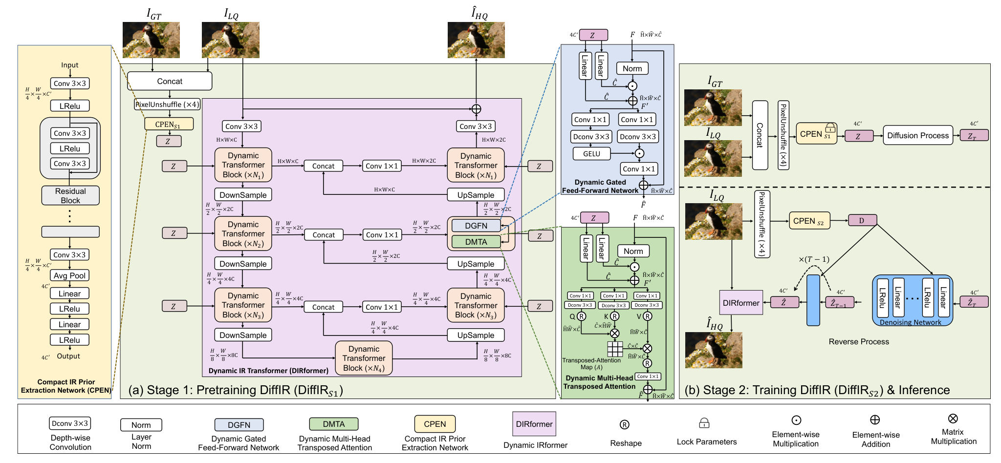
In this paper, we aim to design a DM-based IR network that can fully and efficiently use the powerful distribution mapping abilities of DM to restore images. To this end, we propose DiffIR. Since the transformer can model long-range pixel dependencies, we adopt the transformer blocks as our basic unit of DiffIR. We stack transformer blocks in Unet shape to form Dynamic IRformer (DIRformer) to extract and aggregate multi-level features. We train our DiffIR in two stages: (1) In the first stage (Fig. 2 (a)), we develop a compact IR prior extraction network (CPEN) to extract a compact IR prior representation (IPR) from ground-truth images to guide the DIRformer. Besides, we develop Dynamic Gated Feed-Forward Network (DGFN) and Dynamic Multi-Head Transposed Attention (DMTA) for DIRformer to fully use the IPR. It is notable that CPEN and DIRformer are optimized together. (2) In the second stage (Fig. 2 (b)), we train the DM to directly estimate the accurate IPR from LQ images. Since the IPR is light and only adds details for restoration, our DM can estimate quite an accurate IPR and obtain stable visual results after several iterations.

Apart from the above scheme and architectural novelties, we show the effectiveness of joint optimization. In the second stage, we observe that the estimated IPR may still have minor errors, which will affect the performance of the DIRformer. However, the previous DMs need many iterations, which is unavailable to optimize DM with the decoder together. Since our DiffIR requires few iterations, we can run all iterations and obtain the estimated IPR to optimize with DIRformer jointly. As shown in Fig. 1, our DiffIR achieves SOTA performance consuming much less computation than other DM-based methods (e.g., RePaint [40] and LDM [50]). In particular, DiffIR is 1000 $\times$ more efficient than RePaint. Our main contributions are threefold:

•

We propose DiffIR, a strong, simple, and efficient DM-based baseline for IR. Unlike image synthesis, most pixels of input images in IR are given. Thus, we use the strong mapping abilities of DM to estimate a compact IPR to guide IR, which can improve the restoration efficiency and stability for DM in IR.
•

We propose DGTA and DGFN for Dynamic IRformer to fully exploit the IPR. Different from the previous latent DMs optimizing the denoising network individually, we propose joint optimization of the denoising network and decoder (i.e., DIRformer) to further improve the robustness of estimation errors.
•

Extensive experiments show that the proposed DiffIR can achieve SOTA performance in IR tasks while consuming much less computational resources compared with other DM-based methods.


(a) Inpainting (Tab. 1)	(b) Super-Resolution (Tab. 2)	(c) Motion deblurring (Tab. 3)

Figure 1: The Mult-Adds are measured on 256

\times

256 inputs. Our DiffIR achieves SOTA performance on IR tasks. Notably, LDM [50] and RePaint [40] are DM-based methods, and DiffIR is 1000

\times

more efficient than RePaint while achieving better performance.

Refer to caption — Figure 2: The overview of the proposed DiffIR, which consists of DIRformer, CPEN, and denoising network. DiffIR has two training stages: (a) In the first stage, CPEN_S1 takes the ground-truth image as input and outputs an IPR $\mathbf{Z}$ to guide DIRformer to restore images. We optimize the CPEN_S1 with DiffIR_S1 together to make DiffIR_S1 can fully use extracted IPR. (b) In the second stage, we use the strong data estimation abilities of the DM to estimate the IPR extracted by pretrained CPEN_S1. Notably, we do not input the ground-truth image into CPEN_S2 and denoising networks. In the inference stage, we only use the reverse process of DM.

2 Related Work

Image Restoration. As pioneer works, SRCNN [15], DnCNN [84], and ARCNN [14] adopt compact CNN to achieve impressive performance on IR. After that, CNN-based methods became more popular compared with traditional IR methods. Up to now, researchers have carried out CNN’s study with different perspectives and obtained more elaborate network architecture designs and learning schemes, such as residual block [29, 81, 6], GAN [21, 65, 48], attention [86, 66, 11, 72, 71, 68, 73], knowledge distillation [67], and others [26, 19, 30, 18, 76].

Recently, transformer, a natural language processing model, has gained much popularity in the computer vision community. Compared with CNN, transformers can model global interactions between different regions and achieve state-of-the-art performance. Presently, the transformer has been adopted in numerous vision tasks, such as image recognition [17, 60], segmentation [62, 69, 87, 49], object detection [5, 89], and image restoration [7, 38, 74, 36, 8].

Diffusion Models. Diffusion Models (DMs) [23], have achieved state-of-the-art results in density estimation [31] as well as in sample quality [12]. DMs adopt parameterized Markov chain to optimize the lower variational bound on the likelihood function, which can make them generate more accurate target distribution than other generative models, i.e., GAN. Recently, DM has become increasingly influential in the field of image restoration tasks, such as super-resolution [28, 52] and inpainting [40, 50, 10]. SR3 [52] and SRdiff [35] introduced a DM to image super-resolution and achieved better performance than SOTA GAN-based methods. Besides, Palette [51] is inspired by conditional generation models [44] and proposes a conditional diffusion model for IR. LDM [50] proposes to perform DM on latent space to improve the restoration efficiency. Furthermore, RePaint [40] designs an improved denoising strategy by resampling iterations in DM for inpainting. However, these DM-based IR methods directly use the paradigm of DM in image synthesis. However, most of the pixels in IR are given, and it is unnecessary to perform DM on whole images or feature maps. Our DiffIR performs DM on a compact IPR, which can make DM process more efficient and stable for IR.

3 Preliminaries: Diffusion Models

In this paper, we adopt diffusion models (DMs) [23] to generate accurate IR prior representation (IPR). In the training phase, DM methods define a diffusion process that transforms an input image $x_{0}$ to Gaussian noise $x_{T}\sim\mathcal{N}(0,1)$ by $T$ iterations. Each iteration of the diffusion process can be described as follows:

q\left(x_{t}\mid x_{t-1}\right)=\mathcal{N}\left(x_{t};\sqrt{1-\beta_{t}}x_{t-1},\beta_{t}\mathbf{I}\right),\vskip-2.84526pt

(1)

where $x_{t}$ is the noised image at time-step $t$ , $\beta_{t}$ is the predefined scale factor, and $\mathcal{N}$ represents the Gaussian distribution. The Eq. (1) can be further simplified as follows:

q\left(\mathbf{x}_{t}\mid\mathbf{x}_{0}\right)=\mathcal{N}\left(\mathbf{x}_{t};\sqrt{\bar{\alpha}_{t}}\mathbf{x}_{0},\left(1-\bar{\alpha}_{t}\right)\mathbf{I}\right),

(2)

where $\alpha_{t}=1-\beta_{t}$ , $\bar{\alpha}_{t}=\prod_{i=0}^{t}\alpha_{i}$ .

In the inference stage (reverse process), DM methods sample a Gaussian random noise map $x_{T}$ and then gradually denoise $x_{T}$ until it reaches a high-quality output $x_{0}$ :

p\left(\mathbf{x}_{t-1}\mid\mathbf{x}_{t},\mathbf{x}_{0}\right)=\mathcal{N}\left(\mathbf{x}_{t-1};\boldsymbol{\mu}_{t}\left(\mathbf{x}_{t},\mathbf{x}_{0}\right),\sigma_{t}^{2}\mathbf{I}\right),

(3)

where mean $\boldsymbol{\mu}_{t}\left(\mathbf{x}_{t},\mathbf{x}_{0}\right)=\frac{1}{\sqrt{\alpha_{t}}}\left(\mathbf{x}_{t}-\epsilon\frac{1-\alpha_{t}}{\sqrt{1-\bar{\alpha}_{t}}}\right)$ and variance $\sigma_{t}^{2}=\frac{1-\bar{\alpha}_{t-1}}{1-\bar{\alpha}_{t}}\beta_{t}$ . $\epsilon$ indicates the noise in $x_{t}$ , which is the only uncertain variable in the reverse process. DMs adopt a denoising network $\epsilon_{\theta}(x_{t},t)$ to estimate $\epsilon$ . To train $\epsilon_{\theta}(x_{t},t)$ , given a clean image $x_{0}$ , DMs randomly sample a time step $t$ and a noise $\epsilon\sim\mathcal{N}(0,\mathbf{I})$ to generate noisy images $x_{t}$ according to Eq. (2). Then, DMs optimize the network parameters $\theta$ of $\epsilon_{\theta}$ following [23]:

\nabla_{\boldsymbol{\theta}}\left\|\epsilon-\epsilon_{\boldsymbol{\theta}}\left(\sqrt{\bar{\alpha}_{t}}\mathrm{x}_{0}+\epsilon\sqrt{1-\bar{\alpha}_{t}},t\right)\right\|_{2}^{2}.

(4)

4 Methodology

Traditional DMs [54, 50, 40] require a large number of iterations, computational resources, and model parameters to generate accurate and realistic images or latent feature maps. Although DMs achieve impressive performance in generating images from scratch (image synthesis), it is a waste of computational resources to directly apply the DM paradigm of image synthesis to IR. Since most pixels and information in IR are given, performing DMs on whole images or feature maps not only spends a lot of iterations and computation but also is easy to generate more artifacts. Overall, DMs have strong data estimation ability, but applying the existing DM paradigm in image synthesis to IR is inefficient. To address the issue, we propose an efficient DM for IR (i.e., DiffIR), which adopts DM to estimate a compact IPR to guide the network to restore images. Since the IPR is quite light, the model size and iteration of DiffIR can be largely reduced to generate more accurate estimations compared with traditional DM.

In this section, we present our DiffIR. As shown in Fig. 2, DiffIR mainly consists of a compact IR prior extraction network (CPEN), dynamic IRformer (DIRformer), and denoising network. We train DiffIR in two stages, including pretraining DiffIR and training the diffusion model. In the following sections, we first introduce the pretraining DiffIR in Sec. 4.1. Then, we provide the details of the training efficient DM for DiffIR in Sec. 4.2.

4.1 Pretrain DiffIR

Before introducing pretraining DiffIR, we would like to introduce two networks in the first stage, including a compact IR prior extraction network (CPEN) and a dynamic IRformer (DIRformer). The structure of CPEN is shown in Fig. 2 yellow box, which is mainly stacked with residual blocks and linear layers to extract the compact IR prior representation (IPR). After that, DIRformer can use the extracted IPR to restore LQ images. The structure of the DIRformer is shown in Fig. 2 pink box, which is stacked with dynamic transformer blocks in the Unet shape. The dynamic transformer blocks consist of dynamic multi-head transposed attention (DMTA, Fig. 2 green box) and dynamic gated feed-forward network (DGFN, Fig. 2 nattier blue box), which can use IPR as dynamic modulation parameters to add restoration details into feature maps.

In the pretraining (Fig. 2 (a)), we train CPEN_S1 and DIRformer together. Specifically, we first concatenate ground-truth and LQ images together and use the PixelUnshuffle operation to downsample them to obtain the input for CPEN_S1. Then, CPEN_S1 extract the IPR $\mathbf{Z}\in\mathbb{R}^{4C^{\prime}}$ as:

\mathbf{Z}=\operatorname{CPEN_{S1}}(\operatorname{PixelUnshuffle}(\operatorname{Concat}(I_{GT},I_{LQ}))).

(5)

Then IPR $\mathbf{Z}$ is sent into DGFN and DMTA of DIRformer as dynamic modulation parameters to guide restoration:

\mathbf{F^{\prime}}=W_{l}^{1}\mathbf{Z}\odot\operatorname{Norm}(\mathbf{F})+W_{l}^{2}\mathbf{Z},

(6)

where $\odot$ indicates element-wise multiplication, $\operatorname{Norm}$ denotes layer normalization [2], $W_{l}$ represents linear layer, $\mathbf{F}$ and $\mathbf{F^{\prime}}\in\mathbb{R}^{\hat{H}\times\hat{W}\times\hat{C}}$ are input and output feature maps respectively, and $W_{l}^{1}\mathbf{Z},W_{l}^{2}\mathbf{Z}\in\mathbb{R}^{\hat{C}}$ .

Then, we aggregate global spatial information in DMTA. Specifically, $\mathbf{F^{\prime}}$ is projected into query $\mathbf{Q}=W_{d}^{Q}W_{c}^{Q}\mathbf{F^{\prime}}$ , key $\mathbf{K}=W_{d}^{K}W_{c}^{K}\mathbf{F^{\prime}}$ , and value $\mathbf{V}=W_{d}^{V}W_{c}^{V}\mathbf{F^{\prime}}$ , where $W_{c}$ is the $1\times 1$ point-wise convolution and $W_{d}$ is the $3\times 3$ depth-wise convolution. Next, we reshape the query $\hat{\mathbf{Q}}\in\mathbb{R}^{\hat{H}\hat{W}\times\hat{C}}$ , key $\hat{\mathbf{K}}\in\mathbb{R}^{\hat{C}\times\hat{H}\hat{W}}$ , and value $\hat{\mathbf{V}}\in\mathbb{R}^{\hat{H}\hat{W}\times\hat{C}}$ . After that, we perform dot-product between $\hat{\mathbf{Q}}$ and $\hat{\mathbf{K}}$ generates a transposed-attention map $\mathbf{A}$ of size $\mathbb{R}^{\hat{C}\times\hat{C}}$ , which is more efficient than regular attention map of size $\mathbb{R}^{\hat{H}\hat{W}\times\hat{H}\hat{W}}$ . The overall process of DMTA can be described as follows:

\vskip-2.84526pt\hat{\mathbf{F}}=W_{c}\hat{\mathbf{V}}\cdot\operatorname{Softmax}(\hat{\mathbf{K}}\cdot\hat{\mathbf{Q}}/\gamma)+\mathbf{F},

(7)

where $\gamma$ is a learnable scaling parameter. As conventional multi-head self attention [17, 7] did, we separate channels to multi-head and calculate attention maps.

Next, in DGFN, we aggregate local features. We use $1\times 1$ Conv to aggregate information from different channels and adopt $3\times 3$ depth-wise Conv to aggregate information from spatially neighboring pixels. Besides, we adopt the gating mechanism to enhance information encoding. The overall process of DGFN is defined as:

\mathbf{\hat{F}}=\operatorname{GELU}\left(W_{d}^{1}W_{c}^{1}\mathbf{F^{\prime}}\right)\odot W_{d}^{2}W_{c}^{2}\mathbf{F^{\prime}}+\mathbf{F}.

(8)

We train CPEN_S1 and DIRformer together, which can make DIRformer fully use the IPR extracted by CPEN_S1 for restoration. The training loss is defined as follows:

L_{rec}=\left\|I_{GT}-\hat{I}_{HQ}\right\|_{1},\vskip-5.69054pt

(9)

where $I_{GT}$ and $\hat{I}_{HQ}$ are the ground-truth and restored HQ images, respectively. $\|\cdot\|_{1}$ denotes the $L_{1}$ norm. If some works emphasize visual quality, such as inpainting and SISR, we can further add perceptual loss and adversarial loss. More details are provided in supplementary materials.

4.2 Diffusion Models for Image Restoration

In the second stage (Fig. 2 (b)), we exploit the strong data estimation ability of the DM to estimate IPR. Specifically, we use the pretrained CPEN_S1 to capture the IPR $\mathbf{Z}\in\mathbb{R}^{4C^{\prime}}$ . After that, we apply the diffusion process on $\mathbf{Z}$ to sample $\mathbf{Z}_{T}\in\mathbb{R}^{4C^{\prime}}$ , which can be described as:

q\left(\mathbf{Z}_{T}\mid\mathbf{Z}\right)=\mathcal{N}\left(\mathbf{Z}_{T};\sqrt{\bar{\alpha}_{T}}\mathbf{Z},\left(1-\bar{\alpha}_{T}\right)\mathbf{I}\right),

(10)

where $T$ is the total number of iterations, $\bar{\alpha}$ and $\alpha$ are defined in Eqs. (1) and (2) (i.e., $\bar{\alpha}_{T}=\prod_{i=0}^{T}\alpha_{i}$ ).

In the reverse process, since IPR is compact, DiffIR_S2 can use much fewer iterations and smaller model size to obtain quite good estimations than traditional DMs [50, 40]. Since traditional DMs have huge computational costs in iterations, they have to randomly sample a time-step $t\in[1,T]$ and merely optimize the denoising network at that time step (Eqs. (1), (2), (3), and (4)). The lack of joint training of the denoising network and decoder (i.e., DIRformer) means the minor error of estimations caused by the denoising network would make the DIRformer cannot achieve its potential. By contrast, DiffIR starts from $T$ -th time step (Eq. (10)) and runs all denoising iterations (Eq. (11)) to obtain $\mathbf{\hat{Z}}$ and send it to DIRformer for joint optimization.

\mathbf{\hat{Z}}_{t-1}=\frac{1}{\sqrt{\alpha_{t}}}\left(\mathbf{\hat{Z}}_{t}-\epsilon\frac{1-\alpha_{t}}{\sqrt{1-\bar{\alpha}_{t}}}\right),\vskip-2.84526pt

(11)

where $\epsilon$ indicates the same noise, and we use the CPEN_S2 and denoising network to predict noise as Eq. (3). It is notable that, different from traditional DMs in Eq. (3), our DiffIR_S2 delete the variance estimation and find it helpful for accurate IPR estimation and better performance (Sec. 6).

In the reverse process of DM, we first use CPEN_S2 to obtain a conditional vector $\mathbf{D}\in\mathbb{R}^{4C^{\prime}}$ from LQ images:

\vskip-2.84526pt\mathbf{D}=\operatorname{CPEN_{S2}}(\operatorname{PixelUnshuffle}(I_{LQ})),

(12)

where CPEN_S2 has the same structure as CPEN_S1 except the input dimension of the first convolution. Then, we use the denoising network $\epsilon_{\theta}$ to estimate noise in each time step $t$ as $\epsilon_{\theta}(\operatorname{Concat}(\mathbf{\hat{Z}}_{t},t,\mathbf{D}))$ . The estimated noise is substituted into Eq. (11) to obtain $\mathbf{\hat{Z}}_{t-1}$ to start the next iteration.

Then, after $T$ times iterations, we obtain the final estimated IPR $\mathbf{\hat{Z}}\in\mathbb{R}^{4C^{\prime}}$ . We joint train CPEN_S2, denoising network, and DIRformer using $\mathcal{L}_{all}$ :

\vskip-2.84526pt\mathcal{L}_{diff}=\frac{1}{4C^{\prime}}\sum_{i=1}^{4C^{\prime}}\left|\hat{\mathbf{Z}}(i)-\mathbf{Z}(i)\right|,\mathcal{L}_{all}=\mathcal{L}_{rec}+\mathcal{L}_{diff},

(13)

where we can further add perceptual loss and adversarial loss in $\mathcal{L}_{all}$ for better visual quality as Eq. (9).

In the inference stage, we only use the reverse diffusion process (the bottom part of Fig. 2 (b)). CPEN_S2 extracts a conditional vector $\mathbf{D}$ from LQ images, and we randomly sample a Gaussian noise $\mathbf{\hat{Z}}_{T}$ . Denoising network utilizes the $\mathbf{\hat{Z}}_{T}$ and $\mathbf{D}$ to estimate IPR $\mathbf{\hat{Z}}$ after $T$ iterations. After that, DIRformer exploits the IPR to restore LQ images.

Table 1: Quantitative comparison (FID/LPIPS) for inpainting on benchmark datasets. Best and second best performance are marked in bold and underlined, respectively. The bottom three methods marked in gray adopt the diffusion model.

Method	#Params (M)	Places [88] (512 $\times$ 512)				CelebA-HQ [27] (256 $\times$ 256)
		Narrow Masks		Wide Masks		Narrow Masks		Wide Masks
		FID $\downarrow$	LPIPS $\downarrow$	FID $\downarrow$	LPIPS $\downarrow$	FID $\downarrow$	LPIPS $\downarrow$	FID $\downarrow$	LPIPS $\downarrow$
EdgeConnect [46]	22	1.3421	0.1106	8.4866	0.1594	6.9566	0.0922	7.8346	0.1149
ICT [61]	150	-	-	-	-	8.4977	0.0982	9.8794	0.1196
LaMa [57]	27	0.6340	0.0898	2.2494	0.1339	5.3889	0.0806	5.7023	0.0951
LDM [50]	215	-	-	2.1500	0.1440	-	-	-	-
RePaint [40]	607	-	-	-	-	4.7395	0.0890	5.4881	0.1094
DiffIR_S2 (Ours)	26	0.4913	0.0758	1.9788	0.1306	4.5967	0.0769	5.1440	0.0918

5 Experiments

5.1 Experiment Settings

We apply our method to three typical IR tasks separately: (a) inpainting, (b) image super-resolution (SR), (c) single-image motion deblurring. Our DiffIR adopts a 4-level encoder-decoder structure. From level- $1$ to level- $4$ , the attention heads in DMTA are $[1,2,4,8]$ , and the number of channels is $[48,96,192,384]$ . Additionally, in all IR tasks, we tune the number of dynamic transformer blocks in DIRformer to compare DiffIR with the SOTA methods in similar parameters and computational costs. Specifically, from level-1 to level-4, we set the number of dynamic transformer blocks to $[1,1,1,9]$ , $[13,1,1,1]$ , and $[3,5,6,6]$ for inpainting, SR, and deblurring, respectively. In addition, following previous works [40, 50], we introduce adversarial loss and perceptual loss for inpainting and SR. The number of channels $C^{\prime}$ of CPEN is set to $64$ .

In training the diffusion model, total timesteps $T$ are set to $4$ , and $\beta_{t}$ in Eq. (11) ( $\alpha_{t}=1-\beta_{t}$ ) linearly increase from $\beta_{1}=0.1$ to $\beta_{T}=0.99$ . We train models with Adam optimizer ( $\beta_{1}=0.9$ , $\beta_{2}=0.99$ ). More details are presented in the supplementary material.

Table 2: Quantitative comparison ( LPIPS/DISTS). for Single image super-resolution on benchmark datasets. Best and second best performance are marked in bold and underlined, respectively. The bottom two methods marked in gray adopt the diffusion model.

Method	Set14 [77]		Urban100 [25]		Manga109 [43]		General100 [16]		DIV2K100 [1]
Method	PSNR $\uparrow$	LPIPS $\downarrow$	PSNR $\uparrow$	LPIPS $\downarrow$	PSNR $\uparrow$	LPIPS $\downarrow$	PSNR $\uparrow$	LPIPS $\downarrow$	PSNR $\uparrow$	LPIPS $\downarrow$
SFTGAN [64]	26.74	0.1313	24.34	0.1343	28.17	0.0716	29.16	0.0947	28.09	0.1331
SRGAN [34]	26.84	0.1327	24.41	0.1439	28.11	0.0707	29.33	0.0964	28.17	0.1257
ESRGAN [65]	26.59	0.1241	24.37	0.1229	28.41	0.0649	29.43	0.0879	28.18	0.1154
USRGAN [80]	27.41	0.1347	24.89	0.1330	28.75	0.0630	30.00	0.0937	28.79	0.1325
SPSR [42]	26.86	0.1207	24.80	0.1184	28.56	0.0672	29.42	0.0862	28.18	0.1099
BebyGAN [37]	27.09	0.1157	25.23	0.1096	29.19	0.0529	29.95	0.0778	28.62	0.1022
LDM [50]	25.62	0.2034	23.36	0.1816	25.87	0.1321	27.17	0.1655	26.66	0.1939
SRdiff [35]	27.14	0.1450	25.12	0.1379	28.67	0.0665	29.83	0.1009	28.58	0.1293
DiffIR_S2 (Ours)	27.73	0.1117	26.05	0.1007	30.32	0.0463	30.58	0.0717	29.13	0.0871

5.2 Evaluation on Inpainting

We train and validate our DiffIR_S2 on inpainting using the same settings of LaMa [57]. Specifically, we train our DiffIR with the batch size of 30 and patch size of 256 on Places-Standard [88] and CelebA-HQ [27] datasets, respectively. We compare our DiffIR_S2 with SOTA inpainting methods (ICT [61], LaMa [57], and RePaint [40]) using LPIPS [85] and FID [22] on validation datasets.

The quantitative results are shown in Tab. 1 and Fig. 1 (a). We can see that our DiffIR_S2 significantly outperforms other methods. Specifically, our DiffIR_S2 surpasses competitive method LaMa by a FID margin of up to 0.2706 and 0.5583 with wide masks on Places and CelebA-HQ consuming similar total numbers of parameters and Mult-Adds. Furthermore, compared with DM based method RePaint [50], our DiffIR_S2 can achieve better performance while merely consuming $4.3\%$ parameters and $0.1\%$ computational resources. This indicates that DiffIR can fully and efficiently use the data estimation ability of DM for IR.

The qualitative results are shown in Fig. 3. Our DiffIR_S2 can produce more realistic and reasonable structures and details than other competitive inpainting methods. More qualitative results are provided in the supplementary material.

5.3 Evaluation on Image Super-Resolution

We train and validate our DiffIR_S2 on image super-resolution. Specifically, we train DiffIR_S2 on DIV2K [1] (800 images) and Flickr2K [59] (2650 images) datasets for $4\times$ super-resolution. The batch sizes are set to 64, and the LQ patch sizes are 64 $\times$ 64. We evaluate our DiffIR_S2 and other SOTA GAN-based SR methods on five benchmarks (Set5 [3], Set14 [77], General100 [16], Urban100 [25], and DIV2K100 [1]) using LPIPS [85] and PSNR.

Tab. 2 and Fig. 1 (b) show the performance and Mult-Adds comparsion of DiffIR_S2 with SOTA GAN-based SR methods: SFTGAN [64], SRGAN [34], ESRGAN [65], USRGAN [80], SPSR [42], and BebyGAN [37]. We can see that DiffIR_S2 achieves the best performance. Compared with the competitive SR method BebyGAN, our DiffIR_S2 surpasses it by LPIPS margin of up to 0.0151 and 0.0089 on DIV2K100 and Urban100 while merely consuming $63\%$ computational resources. Moreover, it is notable that DiffIR_S2 significantly outperforms DM-based method LDM while consuming $2\%$ computational resources.

The qualitative results are shown in Fig. 4. DiffIR_S2 achieves the best visual quality containing more realistic details. These visual comparisons are consistent with the quantitative results, showing the superiority of DiffIR. DiffIR can efficiently use the powerful DM to restore images. More visual results are given in supplementary material.

Table 3: Quantitative comparison for Single image motion deblurring on benchmark datasets. Best and second best performance are marked in bold and underlined, respectively.

Method	GoPro [45]		HIDE [53]
Method	PSNR $\uparrow$	SSIM $\uparrow$	PSNR $\uparrow$	SSIM $\uparrow$
Xu et al. [70]	21.00	0.741	-	-
DeblurGAN [32]	28.70	0.858	24.51	0.871
Nah et al. [45]	29.08	0.914	25.73	0.874
Zhang et al. [79]	29.19	0.931	-	-
DeblurGAN-v2 [33]	29.55	0.934	26.61	0.875
SRN [58]	30.26	0.934	28.36	0.915
Gao et al. [20]	30.90	0.935	29.11	0.913
DBGAN [83]	31.10	0.942	28.94	0.915
MT-RNN [47]	31.15	0.945	29.15	0.918
DMPHN [78]	31.20	0.940	29.09	0.924
Suin et al. [56]	31.85	0.948	29.98	0.930
MIMO-Unet+ [9]	32.45	0.957	29.99	0.930
IPT [7]	32.52	-	-	-
MPRNet [75]	32.66	0.959	30.96	0.939
Restormer [74]	32.92	0.961	31.22	0.942
DiffIR_S2 (Ours)	33.20	0.963	31.55	0.947

5.4 Evaluation on Image Motion Deblurring

We train DiffIR on GoPro [45] dataset for image motion deblurring and evaluate DiffIR on two classic benchmarks (GoPro, HIDE [53]). We compare DiffIR_S2 with the state-of-the-art image motion deblurring methods, including Restormer [74], MPRNet [75], and IPT [7].

The quantitative results (PSNR and SSIM) are shown in Tab. 3, and the Mult-Adds are shown in Fig. 1 (c). We can see that our DiffIR_S2 outperforms other motion deblurring methods. Specifically, DiffIR_S2 surpasses IPT and MIMI-Unet+ by 0.68 dB and 0.54 dB on GoPro, respectively. Furthermore, DiffIR_S2 surpasses Restormer by 0.28 dB and 0.33 dB on GoPro and HIDE datasets separately, only consuming $78\%$ computational resources. This demonstrates the effectiveness of DiffIR.

The qualitative results are shown in Fig. 5, and our DiffIR_S2 has the best visual quality containing more realistic details close to corresponding HQ images. More qualitative results are provided in the supplementary material.

6 Ablation Study

Efficient diffusion model for image restoration. In this part, we validate the effectiveness of the components in DiffIR, such as DM, training schemes for DM, and whether inserting variance noise in DM (Tab. 4).

(1) DiffIR_S2-V3 is actually the DiffIR_S2 adopted in Tab. 1, and DiffIR_S1 is the first stage pretraining network with ground-truth images as inputs. Comparing DiffIR_S1 and DiffIR_S2-V3, we can see that DiffIR_S2-V3 has quite similar LPIPS with DiffIR_S1, which means that DM has powerful data modeling ability to predict accurate IPR.

(2) To further demonstrate the effectiveness of DM, we cancel using DM in DiffIR_S2-V3 to obtain DiffIR_S2-V1. Comparing DiffIR_S2-V1 and DiffIR_S2-V3, we can see that DiffIR_S2-V3 (using DM) significantly outperform DiffIR_S2-V1. That means the IPR learned by DM can effectively guide DIRformer to restore LQ images.

(3) To explore the better training schemes for DM, we compare two training schemes: traditional DM optimization and our proposed joint optimization. Since traditional DM [50, 54] requires many iterations to estimate large images or feature maps, they have to adopt traditional DM optimization by randomly sampling a timestep to optimize the denoising network, which cannot optimize with the later decoder (i.e., DIRformer in our paper). Since DiffIR merely uses DM to estimate a compact one-dimensional vector IPR, we can use several times iterations to obtain quite accurate results. Therefore, we can adopt joint optimization by running all iterations of the denoising network to obtain IPR to optimize with DIRformer jointly. Comparing DiffIR_S2-V2 and DiffIR_S2-V3, DiffIR_S2-V3 significantly surpass the DiffIR_S2-V2, which demonstrates the effectiveness of our proposed joint optimization for training DM. That is because the DM’s minor estimation error in IPR may lead to the performance drop of the DIRformer. Training DM and DIRformer jointly can address this problem.

(4) In traditional DM methods, they will insert variance noise in the reverse DM process (Eq. (3)) to generate more realistic images. Different from traditional DM predicting images or feature maps, we use DM to estimate IPR. In DiffIR_S2-V4, we insert noise in the reverse DM process. As we can see, DiffIR_S2-V3 achieve better performance than DiffIR_S2-V4. That means it is better to cancel inserting noise to guarantee the accuracy of the estimated IPR.

Table 4: FID results evaluated on CelebA-HQ for inpainting. The performance and Mult-Adds are measured on an LQ size of 256

\times

256.

Method	Mult-Adds (G)	GT	DM	Training Schemes		Inserting Noise	CelebA-HQ
Method	Mult-Adds (G)	GT	DM	Traditional DM Optimization	Joint Optimization	Inserting Noise	CelebA-HQ
DiffIR_S1	47.97	✓	✗	✗	✗	✗	4.8045
DiffIR_S2-V1	51.63	✗	✗	✗	✗	✗	5.6782
DiffIR_S2-V2	51.63	✗	✓	✓	✗	✗	5.9766
DiffIR_S2-V3 (Ours)	51.63	✗	✓	✗	✓	✗	5.1440
DiffIR_S2-V4	51.63	✗	✓	✗	✓	✓	5.1937

Table 5: DM loss functions comparison (FID) in inpainting.

Loss	$\mathcal{L}_{diff}$ (Eq. (13))	$\mathcal{L}_{2}$ (Eq. (14))	$\mathcal{L}_{kl}$ (Eq. (15))
CelebA-HQ $\downarrow$	5.1440	5.1837	5.2365

The loss functions for DM. We explore which loss function is best to guide the denoising network and CPEN_S2 to learn to estimate accurate IPR from LQ images. Here, we define three loss functions. (1) We define $\mathcal{L}_{diff}$ for optimization (Eq. (13)). (2) We adopt $\mathcal{L}_{2}$ (Eq. (14)) to measure estimation error. (3) We use the Kullback Leibler divergence to measure distribution similarity ( $\mathcal{L}_{kl}$ , Eq. (15)).

\vskip-5.69054pt\mathcal{L}_{2}=\frac{1}{4C^{\prime}}\sum_{i=1}^{4C^{\prime}}\left(\hat{\mathbf{Z}}(i)-\mathbf{Z}(i)\right)^{2},

(14)

\displaystyle\mathcal{L}_{kl}

\displaystyle=\sum_{i=1}^{4C^{\prime}}\mathbf{Z}_{norm}(i)\log\left(\frac{\mathbf{Z}_{norm}(i)}{\hat{\mathbf{Z}}_{norm}(i)}\right),

(15)

where $\hat{\mathbf{Z}}$ and $\mathbf{Z}\in\mathbb{R}^{4C^{\prime}}$ are IPRs extracted by DiffIR_S1 and DiffIR_S2 respectively. $\hat{\mathbf{Z}}_{norm}$ and $\mathbf{Z}_{norm}\in\mathbb{R}^{4C^{\prime}}$ are normalized with softmax operation of $\hat{\mathbf{Z}}$ and $\mathbf{Z}$ separately. We apply these three loss functions on DiffIR_S2 separately to learn to directly estimate the accurate IPR from LQ images. Then, we evaluate them on CelebA-HQ in the inpainting task. The results are shown in Tab. 5. We can see that the performance of $\mathcal{L}_{diff}$ is better than $\mathcal{L}_{2}$ and $\mathcal{L}_{kl}$ .

Impact of the number of iterations. In this part, we explore how the number of iterations in DM affects the performance of DiffIR_S2. We set different number of iterations in DiffIR_S2 and tune the $\beta_{t}$ ( $\alpha_{t}=1-\beta_{t}$ ) in Eq. (10) to make $\mathbf{Z}$ be Gaussian noise $\mathbf{Z}_{T}\sim\mathcal{N}(0,1)$ after diffusion process (i.e., $\bar{\alpha}_{T}\rightarrow 0$ ). The results are shown in Fig. 6. As iterations increase to 3, the performance of DiffIR_S2 will significantly improve. As the number of iteration is larger than 4, DiffIR_S2 almost keep stable, which means it reaches the upper bound. Besides, we can see that our DiffIR_S2 has more quick convergence speed than traditional DM (requiring more than 200 iterations). That is because we merely perform DM on IPR (a compact one-dimensional vector).

Figure 6: Ablation study of the number of iterations in DM.

7 Conclusion

Traditional DMs achieve impressive performance in image synthesis. Different from image synthesis generating each pixel from scratch, IR gives an LQ image as a reference. Thus, it is inefficient to directly apply the traditional DM paradigm to IR. In this paper, we propose an efficient diffusion model for IR (i.e., DiffIR), consisting of CPEN, DIRformer, and denoising network. Specifically, we first input ground-truth image into CPEN_S1 to generate a compact IPR to guide DIRformer. After that, we train DM to estimate the IPR extracted by CPEN_S1. Compared with traditional DMs, our DiffIR can use much fewer iterations than traditional DMs to obtain accurate estimations and reduce artifacts in restored images. Furthermore, thanks to the few iterations, our DiffIR can adopt joint optimization of CPEN_S2, DIRformer, and denoising network to reduce the influence of estimation error. Extensive experiments show that DiffIR can achieve a general SOTA IR performance.

References

[1] Eirikur Agustsson and Radu Timofte. Ntire 2017 challenge on single image super-resolution: Dataset and study. In CVPRW, 2017.
[2] Jimmy Lei Ba, Jamie Ryan Kiros, and Geoffrey E Hinton. Layer normalization. arXiv preprint arXiv:1607.06450, 2016.
[3] Marco Bevilacqua, Aline Roumy, Christine Guillemot, and Marie line Alberi Morel. Low-complexity single-image super-resolution based on nonnegative neighbor embedding. In BMVC, 2012.
[4] Jianrui Cai, Hui Zeng, Hongwei Yong, Zisheng Cao, and Lei Zhang. Toward real-world single image super-resolution: A new benchmark and a new model. In ICCV, 2019.
[5] Nicolas Carion, Francisco Massa, Gabriel Synnaeve, Nicolas Usunier, Alexander Kirillov, and Sergey Zagoruyko. End-to-end object detection with transformers. In ECCV, 2020.
[6] Lukas Cavigelli, Pascal Hager, and Luca Benini. Cas-cnn: A deep convolutional neural network for image compression artifact suppression. In IJCNN, 2017.
[7] Hanting Chen, Yunhe Wang, Tianyu Guo, Chang Xu, Yiping Deng, Zhenhua Liu, Siwei Ma, Chunjing Xu, Chao Xu, and Wen Gao. Pre-trained image processing transformer. In CVPR, 2021.
[8] Liangyu Chen, Xiaojie Chu, Xiangyu Zhang, and Jian Sun. Simple baselines for image restoration. In ECCV, 2022.
[9] Sung-Jin Cho, Seo-Won Ji, Jun-Pyo Hong, Seung-Won Jung, and Sung-Jea Ko. Rethinking coarse-to-fine approach in single image deblurring. In ICCV, 2021.
[10] Hyungjin Chung, Byeongsu Sim, and Jong Chul Ye. Come-closer-diffuse-faster: Accelerating conditional diffusion models for inverse problems through stochastic contraction. In CVPR, 2022.
[11] Tao Dai, Jianrui Cai, Yongbing Zhang, Shu-Tao Xia, and Lei Zhang. Second-order attention network for single image super-resolution. In CVPR, 2019.
[12] Prafulla Dhariwal and Alexander Nichol. Diffusion models beat gans on image synthesis. NeurIPS, 2021.
[13] Keyan Ding, Kede Ma, Shiqi Wang, and Eero P Simoncelli. Image quality assessment: Unifying structure and texture similarity. TPAMI, 2020.
[14] Chao Dong, Yubin Deng, Chen Change Loy, and Xiaoou Tang. Compression artifacts reduction by a deep convolutional network. In ICCV, 2015.
[15] Chao Dong, Chen Change Loy, Kaiming He, and Xiaoou Tang. Image super-resolution using deep convolutional networks. TPAMI, 2015.
[16] Chao Dong, Chen Change Loy, and Xiaoou Tang. Accelerating the super-resolution convolutional neural network. In ECCV, 2016.
[17] Alexey Dosovitskiy, Lucas Beyer, Alexander Kolesnikov, Dirk Weissenborn, Xiaohua Zhai, Thomas Unterthiner, Mostafa Dehghani, Matthias Minderer, Georg Heigold, Sylvain Gelly, et al. An image is worth 16x16 words: Transformers for image recognition at scale. ICLR, 2021.
[18] Xueyang Fu, Menglu Wang, Xiangyong Cao, Xinghao Ding, and Zheng-Jun Zha. A model-driven deep unfolding method for jpeg artifacts removal. TNNLS, 2021.
[19] Xueyang Fu, Zheng-Jun Zha, Feng Wu, Xinghao Ding, and John Paisley. Jpeg artifacts reduction via deep convolutional sparse coding. In ICCV, 2019.
[20] Hongyun Gao, Xin Tao, Xiaoyong Shen, and Jiaya Jia. Dynamic scene deblurring with parameter selective sharing and nested skip connections. In CVPR, 2019.
[21] Ishaan Gulrajani, Faruk Ahmed, Martin Arjovsky, Vincent Dumoulin, and Aaron Courville. Improved training of wasserstein gans. arXiv preprint arXiv:1704.00028, 2017.
[22] Martin Heusel, Hubert Ramsauer, Thomas Unterthiner, Bernhard Nessler, and Sepp Hochreiter. Gans trained by a two time-scale update rule converge to a local nash equilibrium. NeurIPS, 2017.
[23] Jonathan Ho, Ajay Jain, and Pieter Abbeel. Denoising diffusion probabilistic models. NeurIPS, 2020.
[24] Jonathan Ho, Chitwan Saharia, William Chan, David J Fleet, Mohammad Norouzi, and Tim Salimans. Cascaded diffusion models for high fidelity image generation. JMLR, 2022.
[25] Jia-Bin Huang, Abhishek Singh, and Narendra Ahuja. Single image super-resolution from transformed self-exemplars. In CVPR, 2015.
[26] Xixi Jia, Sanyang Liu, Xiangchu Feng, and Lei Zhang. Focnet: A fractional optimal control network for image denoising. In CVPR, 2019.
[27] Tero Karras, Timo Aila, Samuli Laine, and Jaakko Lehtinen. Progressive growing of gans for improved quality, stability, and variation. arXiv preprint arXiv:1710.10196, 2017.
[28] Bahjat Kawar, Michael Elad, Stefano Ermon, and Jiaming Song. Denoising diffusion restoration models. arXiv preprint arXiv:2201.11793, 2022.
[29] Jiwon Kim, Jung Kwon Lee, and Kyoung Mu Lee. Accurate image super-resolution using very deep convolutional networks. In CVPR, 2016.
[30] Yoonsik Kim, Jae Woong Soh, Jaewoo Park, Byeongyong Ahn, Hyun-Seung Lee, Young-Su Moon, and Nam Ik Cho. A pseudo-blind convolutional neural network for the reduction of compression artifacts. TCSVT, 2019.
[31] Diederik Kingma, Tim Salimans, Ben Poole, and Jonathan Ho. Variational diffusion models. NeurIPS, 2021.
[32] Orest Kupyn, Volodymyr Budzan, Mykola Mykhailych, Dmytro Mishkin, and Jiří Matas. Deblurgan: Blind motion deblurring using conditional adversarial networks. In CVPR, 2018.
[33] Orest Kupyn, Tetiana Martyniuk, Junru Wu, and Zhangyang Wang. Deblurgan-v2: Deblurring (orders-of-magnitude) faster and better. In ICCV, 2019.
[34] Christian Ledig, Lucas Theis, Ferenc Huszár, Jose Caballero, Andrew Cunningham, Alejandro Acosta, Andrew Aitken, Alykhan Tejani, Johannes Totz, Zehan Wang, et al. Photo-realistic single image super-resolution using a generative adversarial network. In CVPR, 2017.
[35] Haoying Li, Yifan Yang, Meng Chang, Shiqi Chen, Huajun Feng, Zhihai Xu, Qi Li, and Yueting Chen. Srdiff: Single image super-resolution with diffusion probabilistic models. Neurocomputing, 2022.
[36] Wenbo Li, Zhe Lin, Kun Zhou, Lu Qi, Yi Wang, and Jiaya Jia. Mat: Mask-aware transformer for large hole image inpainting. In CVPR, 2022.
[37] Wenbo Li, Kun Zhou, Lu Qi, Liying Lu, and Jiangbo Lu. Best-buddy gans for highly detailed image super-resolution. In AAAI, 2022.
[38] Jingyun Liang, Jiezhang Cao, Guolei Sun, Kai Zhang, Luc Van Gool, and Radu Timofte. Swinir: Image restoration using swin transformer. In ICCVW, 2021.
[39] Ilya Loshchilov and Frank Hutter. Sgdr: Stochastic gradient descent with warm restarts. ICLR, 2017.
[40] Andreas Lugmayr, Martin Danelljan, Andres Romero, Fisher Yu, Radu Timofte, and Luc Van Gool. Repaint: Inpainting using denoising diffusion probabilistic models. In CVPR, 2022.
[41] Andreas Lugmayr, Martin Danelljan, and Radu Timofte. Ntire 2020 challenge on real-world image super-resolution: Methods and results. In CVPRW, 2020.
[42] Cheng Ma, Yongming Rao, Yean Cheng, Ce Chen, Jiwen Lu, and Jie Zhou. Structure-preserving super resolution with gradient guidance. In CVPR, 2020.
[43] Yusuke Matsui, Kota Ito, Yuji Aramaki, Azuma Fujimoto, Toru Ogawa, Toshihiko Yamasaki, and Kiyoharu Aizawa. Sketch-based manga retrieval using manga109 dataset. Multimedia Tools and Applications, 2017.
[44] Mehdi Mirza and Simon Osindero. Conditional generative adversarial nets. arXiv preprint arXiv:1411.1784, 2014.
[45] Seungjun Nah, Tae Hyun Kim, and Kyoung Mu Lee. Deep multi-scale convolutional neural network for dynamic scene deblurring. In CVPR, 2017.
[46] Kamyar Nazeri, Eric Ng, Tony Joseph, Faisal Z Qureshi, and Mehran Ebrahimi. Edgeconnect: Generative image inpainting with adversarial edge learning. arXiv preprint arXiv:1901.00212, 2019.
[47] Dongwon Park, Dong Un Kang, Jisoo Kim, and Se Young Chun. Multi-temporal recurrent neural networks for progressive non-uniform single image deblurring with incremental temporal training. In ECCV, 2020.
[48] Deepak Pathak, Philipp Krahenbuhl, Jeff Donahue, Trevor Darrell, and Alexei A Efros. Context encoders: Feature learning by inpainting. In CVPR, 2016.
[49] Olivier Petit, Nicolas Thome, Clement Rambour, Loic Themyr, Toby Collins, and Luc Soler. U-net transformer: Self and cross attention for medical image segmentation. In MLMI, 2021.
[50] Robin Rombach, Andreas Blattmann, Dominik Lorenz, Patrick Esser, and Björn Ommer. High-resolution image synthesis with latent diffusion models. In CVPR, 2022.
[51] Chitwan Saharia, William Chan, Huiwen Chang, Chris Lee, Jonathan Ho, Tim Salimans, David Fleet, and Mohammad Norouzi. Palette: Image-to-image diffusion models. In ACM SIGGRAPH, 2022.
[52] Chitwan Saharia, Jonathan Ho, William Chan, Tim Salimans, David J Fleet, and Mohammad Norouzi. Image super-resolution via iterative refinement. TPAMI, 2022.
[53] Ziyi Shen, Wenguan Wang, Xiankai Lu, Jianbing Shen, Haibin Ling, Tingfa Xu, and Ling Shao. Human-aware motion deblurring. In ICCV, 2019.
[54] Jascha Sohl-Dickstein, Eric Weiss, Niru Maheswaranathan, and Surya Ganguli. Deep unsupervised learning using nonequilibrium thermodynamics. In ICML, 2015.
[55] Yang Song, Jascha Sohl-Dickstein, Diederik P Kingma, Abhishek Kumar, Stefano Ermon, and Ben Poole. Score-based generative modeling through stochastic differential equations. ICLR, 2021.
[56] Maitreya Suin, Kuldeep Purohit, and AN Rajagopalan. Spatially-attentive patch-hierarchical network for adaptive motion deblurring. In CVPR, 2020.
[57] Roman Suvorov, Elizaveta Logacheva, Anton Mashikhin, Anastasia Remizova, Arsenii Ashukha, Aleksei Silvestrov, Naejin Kong, Harshith Goka, Kiwoong Park, and Victor Lempitsky. Resolution-robust large mask inpainting with fourier convolutions. In WACV, 2022.
[58] Xin Tao, Hongyun Gao, Xiaoyong Shen, Jue Wang, and Jiaya Jia. Scale-recurrent network for deep image deblurring. In CVPR, 2018.
[59] Radu Timofte, Eirikur Agustsson, Luc Van Gool, Ming-Hsuan Yang, and Lei Zhang. Ntire 2017 challenge on single image super-resolution: Methods and results. In CVPRW, 2017.
[60] Hugo Touvron, Matthieu Cord, Matthijs Douze, Francisco Massa, Alexandre Sablayrolles, and Hervé Jégou. Training data-efficient image transformers & distillation through attention. In ICML, 2021.
[61] Ziyu Wan, Jingbo Zhang, Dongdong Chen, and Jing Liao. High-fidelity pluralistic image completion with transformers. In ICCV, 2021.
[62] Wenhai Wang, Enze Xie, Xiang Li, Deng-Ping Fan, Kaitao Song, Ding Liang, Tong Lu, Ping Luo, and Ling Shao. Pyramid vision transformer: A versatile backbone for dense prediction without convolutions. In ICCV, 2021.
[63] Xintao Wang, Liangbin Xie, Chao Dong, and Ying Shan. Real-esrgan: Training real-world blind super-resolution with pure synthetic data. In ICCV, 2021.
[64] Xintao Wang, Ke Yu, Chao Dong, and Chen Change Loy. Recovering realistic texture in image super-resolution by deep spatial feature transform. In CVPR, 2018.
[65] Xintao Wang, Ke Yu, Shixiang Wu, Jinjin Gu, Yihao Liu, Chao Dong, Yu Qiao, and Chen Change Loy. Esrgan: Enhanced super-resolution generative adversarial networks. In ECCVW, pages 0–0, 2018.
[66] Bin Xia, Yucheng Hang, Yapeng Tian, Wenming Yang, Qingmin Liao, and Jie Zhou. Efficient non-local contrastive attention for image super-resolution. AAAI, 2022.
[67] Bin Xia, Yulun Zhang, Yitong Wang, Yapeng Tian, Wenming Yang, Radu Timofte, and Luc Van Gool. Knowledge distillation based degradation estimation for blind super-resolution. ICLR, 2023.
[68] Chaohao Xie, Shaohui Liu, Chao Li, Ming-Ming Cheng, Wangmeng Zuo, Xiao Liu, Shilei Wen, and Errui Ding. Image inpainting with learnable bidirectional attention maps. In ICCV, 2019.
[69] Enze Xie, Wenhai Wang, Zhiding Yu, Anima Anandkumar, Jose M Alvarez, and Ping Luo. Segformer: Simple and efficient design for semantic segmentation with transformers. NeurIPS, 2021.
[70] Li Xu, Shicheng Zheng, and Jiaya Jia. Unnatural l0 sparse representation for natural image deblurring. In CVPR, 2013.
[71] Zili Yi, Qiang Tang, Shekoofeh Azizi, Daesik Jang, and Zhan Xu. Contextual residual aggregation for ultra high-resolution image inpainting. In CVPR, 2020.
[72] Jiahui Yu, Zhe Lin, Jimei Yang, Xiaohui Shen, Xin Lu, and Thomas S Huang. Generative image inpainting with contextual attention. In CVPR, 2018.
[73] Jiahui Yu, Zhe Lin, Jimei Yang, Xiaohui Shen, Xin Lu, and Thomas S Huang. Free-form image inpainting with gated convolution. In ICCV, 2019.
[74] Syed Waqas Zamir, Aditya Arora, Salman Khan, Munawar Hayat, Fahad Shahbaz Khan, and Ming-Hsuan Yang. Restormer: Efficient transformer for high-resolution image restoration. In CVPR, 2022.
[75] Syed Waqas Zamir, Aditya Arora, Salman Khan, Munawar Hayat, Fahad Shahbaz Khan, Ming-Hsuan Yang, and Ling Shao. Multi-stage progressive image restoration. In CVPR, 2021.
[76] Yanhong Zeng, Jianlong Fu, Hongyang Chao, and Baining Guo. Aggregated contextual transformations for high-resolution image inpainting. IEEE Transactions on Visualization and Computer Graphics, 2022.
[77] Roman Zeyde, Michael Elad, and Matan Protter. On single image scale-up using sparse-representations. In International conference on curves and surfaces, 2010.
[78] Hongguang Zhang, Yuchao Dai, Hongdong Li, and Piotr Koniusz. Deep stacked hierarchical multi-patch network for image deblurring. In CVPR, 2019.
[79] Jiawei Zhang, Jinshan Pan, Jimmy Ren, Yibing Song, Linchao Bao, Rynson WH Lau, and Ming-Hsuan Yang. Dynamic scene deblurring using spatially variant recurrent neural networks. In CVPR, 2018.
[80] Kai Zhang, Luc Van Gool, and Radu Timofte. Deep unfolding network for image super-resolution. In CVPR, 2020.
[81] Kai Zhang, Yawei Li, Wangmeng Zuo, Lei Zhang, Luc Van Gool, and Radu Timofte. Plug-and-play image restoration with deep denoiser prior. TPAMI, 2021.
[82] Kai Zhang, Jingyun Liang, Luc Van Gool, and Radu Timofte. Designing a practical degradation model for deep blind image super-resolution. arXiv preprint arXiv:2103.14006, 2021.
[83] Kaihao Zhang, Wenhan Luo, Yiran Zhong, Lin Ma, Bjorn Stenger, Wei Liu, and Hongdong Li. Deblurring by realistic blurring. In CVPR, 2020.
[84] Kai Zhang, Wangmeng Zuo, Yunjin Chen, Deyu Meng, and Lei Zhang. Beyond a gaussian denoiser: Residual learning of deep cnn for image denoising. TIP, 2017.
[85] Richard Zhang, Phillip Isola, Alexei A Efros, Eli Shechtman, and Oliver Wang. The unreasonable effectiveness of deep features as a perceptual metric. In CVPR, 2018.
[86] Yulun Zhang, Kunpeng Li, Kai Li, Lichen Wang, Bineng Zhong, and Yun Fu. Image super-resolution using very deep residual channel attention networks. In ECCV, 2018.
[87] Sixiao Zheng, Jiachen Lu, Hengshuang Zhao, Xiatian Zhu, Zekun Luo, Yabiao Wang, Yanwei Fu, Jianfeng Feng, Tao Xiang, Philip HS Torr, et al. Rethinking semantic segmentation from a sequence-to-sequence perspective with transformers. In CVPR, 2021.
[88] Bolei Zhou, Agata Lapedriza, Aditya Khosla, Aude Oliva, and Antonio Torralba. Places: A 10 million image database for scene recognition. TPAMI, 2017.
[89] Xizhou Zhu, Weijie Su, Lewei Lu, Bin Li, Xiaogang Wang, and Jifeng Dai. Deformable detr: Deformable transformers for end-to-end object detection. arXiv preprint arXiv:2010.04159, 2020.

Appendix A Appendix

Appendix B Evaluation on Real-world SR

We train and validate our DiffIR_S2 on real-world SR using the same settings of Real-ESRGAN [63]. Specifically, we adopt the same loss functions of Real-ESRGAN [65], which further introduce perceptual loss and adversarial loss to the basic $\mathcal{L}_{1}$ loss. We set the learning rate of the DiffIR_S2 to $2\times 10^{-4}$ . We further validate the effectiveness of DiffIR_S2 on Real-World datasets. For optimization, we use Adam with $\beta_{1}=0.9$ , $\beta_{2}=0.99$ . In both two stages of training, we set the batch size to $64$ , with the input patch size being $64$ . We evaluate all methods on the dataset provided in the challenge of Real-World Super-Resolution: NTIRE2020 Track1 and Tracks [41]. In addition, we also validate our DiffIR on RealSRSet [4]. Since NTIRE2020 Track1 and RealSRSet datasets provide a paired validation set, we use the LPIPS [85], DISTS [13], and PSNR for the evaluation.

The quantitative results are shown in Tab. 6. We can see that DiffIR_S2 outperforms SOTA real-world SR method KDSR_S-GAN on LPIPS, DISTS, and PSNR, consuming fewer computational costs. In addition, we can see that DiffIR_S2 outperforms classic real-world SR method Real-ESRGAN on LPIPS, DISTS, and PSNR, only consuming its $63\%$ Mult-Adds. Furthermore, compared with DM-based LDM [50], DiffIR_S2 achieve much better performance consuming only $2\%$ Mult-Adds.

We also visualize the results on NTIRE2020 Track2, which was captured with smartphones. The qualitative results are shown in Fig. 7. We can see that DiffIR_S2 achieves the best performance.

Table 6: 4

\times

SR quantitative comparison on real-world SR benchmarks. The Mult-Adds are computed based on an LR size of 256

\times

256. Best and second best performance are marked in bold and underlined, respectively. The bottom two methods marked in gray adopt the diffusion model.

Methods	Mult-Adds (T)	RealSRSet [4]			NTIRE2020 Track1 [41]
Methods	Mult-Adds (T)	LPIPS $\downarrow$	DISTS $\downarrow$	PSNR $\uparrow$	LPIPS $\downarrow$	DISTS $\downarrow$	PSNR $\uparrow$
BSRGAN [82]	1.18	0.3648	0.1676	26.90	0.3691	0.1368	26.75
Real-ESRGAN [63]	1.18	0.3629	0.1609	26.07	0.3471	0.1326	26.40
KDSR_s-GAN [67]	0.86	0.3610	0.1627	27.18	0.3198	0.1252	27.12
LDM [50]	37.25	0.4369	0.1982	26.37	0.4763	0.1844	25.68
DiffIR_S2 (Ours)	0.74	0.3527	0.1588	27.65	0.3088	0.1131	27.31

Appendix C Algorithm

The algorithm of DiffIR₂ training is summarized in Alg. 1. The algorithm of DiffIR₂ inference is summarized in Alg. 2.

Algorithm 1 DiffIR_S2 Training

Input: Trained DiffIR_S1 (including CPEN_S1 and DIRformer), $\beta_{t}(t\in[1,T])$ .
Output: Trained DiffIR_S2.

1: Init:

\alpha_{t}=1-\beta_{t}

\bar{\alpha}_{T}=\prod_{i=0}^{T}\alpha_{i}

2: Init: The DIRformer of DiffIR_S2 copies the parameters of trained DiffIR_S1.

3: for

I_{LQ}

I_{GT}

\mathbf{Z}=\operatorname{CPEN_{S1}}(\operatorname{PixelUnshuffle}(\operatorname{Concat}(I_{GT},I_{LQ}))).

(paper Eq. (5))

5: Diffusion Process:

6: We sample

\mathbf{Z}_{T}

q\left(\mathbf{Z}_{T}\mid\mathbf{Z}\right)=\mathcal{N}\left(\mathbf{Z}_{T};\sqrt{\bar{\alpha}_{T}}\mathbf{Z},\left(1-\bar{\alpha}_{T}\right)\mathbf{I}\right)

(i.e., diffusion process. paper Eq. (10))

7: Reverse Process:

\mathbf{\hat{Z}}_{T}=\mathbf{Z}_{T}

\mathbf{D}=\operatorname{CPEN_{S2}}(\operatorname{PixelUnshuffle}(I_{LQ}))

(paper Eq. (12))

10: for

t=T

1

11:

\mathbf{\hat{Z}}_{t-1}=\frac{1}{\sqrt{\alpha_{t}}}\left(\mathbf{\hat{Z}}_{t}-\epsilon_{\theta}(\operatorname{Concat}(\mathbf{\hat{Z}}_{t},t,\mathbf{D}))\frac{1-\alpha_{t}}{\sqrt{1-\bar{\alpha}_{t}}}\right)

(paper Eq. (11))

12: end for

13:

\mathbf{\hat{Z}}=\mathbf{\hat{Z}}_{0}

14:

\hat{I}_{HQ}=\operatorname{DIRformer}(I_{LQ},\mathbf{\hat{Z}})

15: Calculate

\mathcal{L}_{diff}

loss (paper Eq. (13)).

16: end for

17: Output the trained model DiffIR_S2.

Algorithm 2 DiffIR_S2 Inference

Input: Trained DiffIR_S2 (including CPEN_S2 and DIRformer), $\beta_{t}(t\in[1,T])$ , LQ images $I_{LQ}$ .
Output: Restored HQ images $\hat{I}_{HQ}$ .

1: Init:

\alpha_{t}=1-\beta_{t}

\bar{\alpha}_{T}=\prod_{i=0}^{T}\alpha_{i}

2: Reverse Process:

3: Sample

\mathbf{\hat{Z}}_{T}\sim\mathcal{N}(0,1)

\mathbf{D}=\operatorname{CPEN_{S2}}(\operatorname{PixelUnshuffle}(I_{LQ}))

(paper Eq. (12))

5: for

t=T

1

\mathbf{\hat{Z}}_{t-1}=\frac{1}{\sqrt{\alpha_{t}}}\left(\mathbf{\hat{Z}}_{t}-\epsilon_{\theta}(\operatorname{Concat}(\mathbf{\hat{Z}}_{t},t,\mathbf{D}))\frac{1-\alpha_{t}}{\sqrt{1-\bar{\alpha}_{t}}}\right)

(paper Eq. (11))

7: end for

\mathbf{\hat{Z}}=\mathbf{\hat{Z}}_{0}

\hat{I}_{HQ}=\operatorname{DIRformer}(I_{LQ},\mathbf{\hat{Z}})

10: Output restored HQ images

\hat{I}_{HQ}

Appendix D More Training Details on Inpainting

We train our DiffIR for inpainting using the same loss functions of LaMa [57], which further introduce multiple perceptual losses and adversarial loss to the basic $\mathcal{L}_{1}$ loss.

For our experiments on image-inpainting in the paper Sec. 5.2, we used the code of LaMa [57] to generate synthetic masks. In training, we adopt the Adam optimizer with learning rates $0.0002$ and $0.0001$ for DiffIR and discriminator networks, respectively. All models are trained for 1M iterations with a batch size of 30. In addition, we use random crops of size $256\times 256$ to train DiffIR on Places and CelebA-HQ. In testing, we use a fixed set of 2k validation and 30k testing samples from CelebA-HQ [27] and Places [88]. Moreover, we validate DiffIR_S2 on crops of size $512\times 512$ and $256\times 256$ on Places and CelebA-HQ validation datasets, respectively.

Appendix E More Training Details on SR

Compared with DIRformer for other IR tasks, we add a $\times 4$ upsampling network [65] at the end of DIRformer for super-resolution (SR). We train our DiffIR for SR using the same loss functions of ESRGAN [65], which further introduce perceptual loss and adversarial loss to the basic $\mathcal{L}_{1}$ loss.

We train DiffIR for 1M iterations with a batch size of $64$ . In addition, we use random crops of size $256\times 256$ to train DiffIR on DIV2K [1] (800 images) and Flickr2K [59] (2650 images) datasets for 4 $\times$ super-resolution. We train our DiffIR using Adam optimizer with learning rates $0.0002$ and $0.0001$ for DiffIR and discriminator networks, respectively.

Appendix F More Training Details on deblurring

Following previous works in single image motion deblurring [9, 75, 74], we train our DiffIR only using $\mathcal{L}_{1}$ loss for fair comparisons. We train DiffIR for 300K iterations with the initial learning rate $2^{-4}$ gradually reduced to $1^{-6}$ with the cosine annealing [39]. Following previous work [74], we progressively increase patch size and decrease batch size. Specifically, we start training with patch size $128\times 128$ and batch size $64$ . The patch size and batch size pairs are updated to $[(1602,40),(1922,32),(2562,16),(3202,8),(3842,8)]$ at iterations $[92K,156K,204K,240K,276K]$ .

Appendix G More Visual Comparisons on Inpainting

In this section, we provide more qualitative comparisons between our DiffIR_S2 and SOTA inpainting methods (ICT [61], LaMa [57], and RePaint [40]). The results are shown in Fig 8. We can observe that our DiffIR_S2 can produce more realistic and reasonable structures and details than other competitive inpainting methods.

Appendix H More Visual Comparisons on SR

In this section, we provide more qualitative comparisons between our DiffIR_S2 and SOTA GAN-based SR methods. The results are shown in Figs 9 and 10. Our DiffIR_S2 achieves the best visual quality containing more realistic details.

Appendix I More Visual Comparisons on Deblurring

In this section, we provide more qualitative comparisons between our DiffIR_S2 and SOTA image motion deblurring methods. The results are shown in Fig 11. Our DiffIR_S2 has the best visual quality containing more realistic details close to corresponding HQ images.