Contrastive Semi-supervised Learning for Underwater Image Restoration via Reliable Bank
Abstract
Despite the remarkable achievement of recent underwater image restoration techniques, the lack of labeled data has become a major hurdle for further progress. In this work, we propose a mean-teacher based Semi-supervised Underwater Image Restoration (Semi-UIR) framework to incorporate the unlabeled data into network training. However, the naive mean-teacher method suffers from two main problems: (1) The consistency loss used in training might become ineffective when the teacher’s prediction is wrong. (2) Using L1 distance may cause the network to overfit wrong labels, resulting in confirmation bias. To address the above problems, we first introduce a reliable bank to store the “best-ever” outputs as pseudo ground truth. To assess the quality of outputs, we conduct an empirical analysis based on the monotonicity property to select the most trustworthy NR-IQA method. Besides, in view of the confirmation bias problem, we incorporate contrastive regularization to prevent the overfitting on wrong labels. Experimental results on both full-reference and non-reference underwater benchmarks demonstrate that our algorithm has obvious improvement over SOTA methods quantitatively and qualitatively. Code has been released at https://github.com/Huang-ShiRui/Semi-UIR.
1 Introduction
Due to light refraction, absorption and scattering in underwater scenes, images taken in the water usually suffer severely from color distortion, low contrast and blur. Images with these defects tend to be less visually appealing and can potentially hinder the well-functioning of underwater robotic systems. Recently, many deep learning based methods huan1; huan2; huan3; huan4; huan5 have been proposed to address image restoration problems. Numerous efforts have also been devoted to the specific domain of underwater image restoration UIEBD; EUVP-FUnieGan; ucolor; cwr; yin2021fmsnet. Compared with traditional methods that mostly rely on hand-crafted priors, deep learning based solutions are able to deliver superior restoration results due to their data-driven nature.
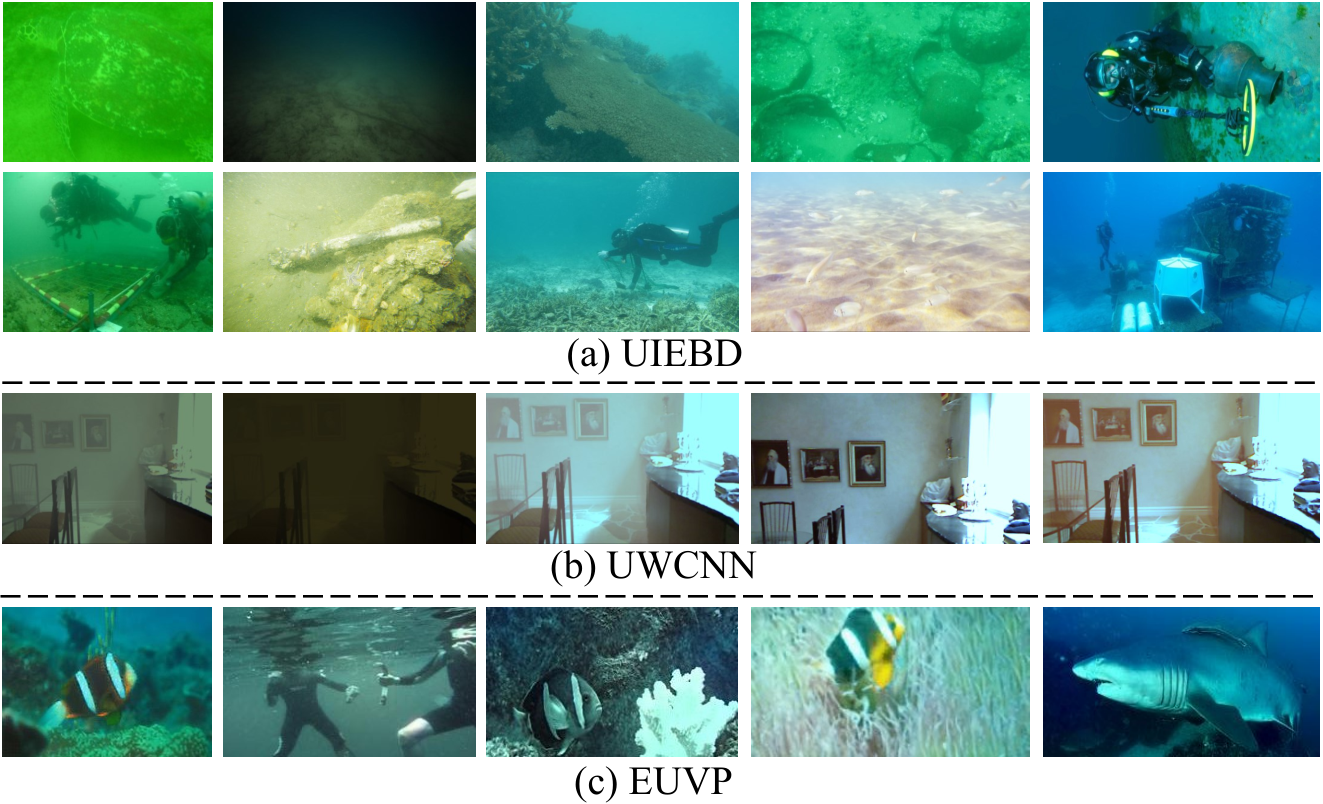
Despite their success, most of deep learning based methods are designed to learn the restoration mapping on paired datasets in a supervised manner. As is known, it is extremely hard, if not impossible, to acquire paired underwater images in real scenes. The existing datasets for underwater image restoration have several non-negligible issues: (1) Lack of real data. A popular way to construct paired datasets is to synthesize underwater images using some physical modelAnwar2019UWCNN or GANEUVP-FUnieGan. However, there is a significant discrepancy between synthesized and real data UWNR. As is shown in Fig. 1, the ambient light and color cast of synthetic data are quite different from the real counterparts. Due to domain shift, models trained on synthetic datasets often exhibit poor generalization in real scenes. Another wayUIEBD is to manually construct pseudo labels by selecting the best results among those produced by traditional algorithms. Inevitably, the quality of the pseudo ground truth is restricted by the restoration capability of traditional algorithms. (2) Limited data size. The current benchmarks only provide a very limited amount of paired data. For example, in UIEBUIEBD, there are only 890 paired underwater images. Models learned on such a small dataset may run the risk of overfitting. In comparison, the standard datasets for image classification, such as ImageNetimagenet, are several orders of magnitude larger in size.
On the other hand, unlabeled underwater images are relatively easy to collect. The challenge is how to make effective use of these unlabeled data. Semi-supervised learning, which capitalizes on both labeled and unlabeled data for model training, is best suited in this kind of scenarios. This motivates us to propose a semi-supervised scheme with the goal of improving the generalization of the resulting model on real-world underwater images. To be specific, we adopt the mean teacher methodtarvainen2017mean as the basis. The mean teacher method finds a way to obtain pseudo labels for unlabeled data and utilizes a consistency loss to improve the accuracy and robustness of the network. Specifically, it constructs a teacher model with improved performance from a student model via the exponential moving average (EMA) strategy. The teacher’s prediction serves as the pseudo label to guide the training of the student. However, it is a non-trivial task to tailor the mean teacher method to the underwater image restoration problem. The reasons are as follows: (1) There is no guarantee that the teacher can consistently outperform the student. Wrong pseudo labels may jeopardize the training of the student network. (2) The commonly used consistency loss is based on L1 distance. The “strict” L1 loss can easily make the model overfit wrong predictions, resulting in confirmation bias.
To address the first issue, we construct a reliable bank to archive the best-ever outputs from the teacher as pseudo labels. The main challenge here is how to determine what are the “best-ever” outputs? Intuitively, non-reference image quality assessment (NR-IQA) can be leveraged to evaluate the quality of each output. However, as noted in berman2020underwater; UIEBD; guo2023uranker, the current NR-IQA metrics for underwater images are, to some extent, inconsistent with human visual perception. To identify the right one for our purpose, we compare several NR-IQA metrics using the monotonicity property as the reliability criterion. Our empirical analysis suggests MUSIQke2021musiq best meets the criterion. For the second issue, we introduce contrastive learning as a supplementary regularization to alleviate overfitting. Unlike those conventional loss functions that are only concerned with how close the outputs and ground truths are, contrastive loss provides additional supervision to prevent the degradation of the outputs. In this sense, contrastive regularization is ideally suited to our semi-supervised learning framework since we only have access to the degraded images in the unlabeled dataset. It enables the model to take advantage of unlabeled data.
In summary, our main contributions are as follows: (1) We propose a mean teacher based semi-supervised underwater image restoration framework named Semi-UIR, which effectively leverages the knowledge from unlabeled data to improve the generalization of the trained model on real-world data. (2) We evaluate teacher outputs by a judiciously chosen NR-IQA metric and build a reliable bank to store best-ever teacher outputs, which ensures the reliability of pseudo-labels. (3) We adopt contrastive loss as a form of regularization to alleviate confirmation bias. (4) Extensive experimental results demonstrate the effectiveness of our proposed methods.
2 Related Work
2.1 Underwater Image Restoration Methods
Traditional underwater image restoration methods can be categorized into model-based and model-agnostic methods. Model-based methodsgaldran2015rcp; peng2018gdcp; berman2020underwater use hand-crafted priors to estimate unknown parameters of underwater imaging modelschechner2004clear, such as transmission and ambient light. In contrast, model-agnostic methods rely on the design of appropriate image enhancement techniques such as CLAHEclahe-mix, Retinexlabmsr, fusionfusion-18 and MMLEMMLE. Despite their success, the traditional methods usually fail to cope with complex real scenes.
Most of early deep learning based underwater image restoration methodswang2019underwater; kar2021zero accomplish the goal by exploiting physical imaging models. Specifically, they make use of neural networks to estimate the transmission and ambient light. However, inaccurate estimation of these parameters hinders such methods from achieving good performance. Recent years have seen many deep learning based methods that directly learn the restoration mapping from the labeled dataset in a supervised manner without resorting to imaging models. UIEBD employs an effective network to fuse three feature maps enhanced by traditional model-agnostic methods. ucolor designs a multi-color space encoder and a transmission-guided decoder by leveraging the ideas from traditional model-based approaches. prwnet proposes a wavelet boost learning strategy, through which features in the frequency domain are utilized for fine detail restoration. EUVP-FUnieGan introduces an end-to-end network based on GAN for the purpose of real-time inference.
2.2 Semi-supervised Learning
In recent years, semi-supervised learning zhu2005semi has played an increasingly important role in tackling computer vision problems. It focuses on making effective use of both labeled and unlabeled data. Many semi-supervised methods have been developed, such as mean teachertarvainen2017mean, virtual adversarial learningmiyato2018virtual and FixMatchsohn2020fixmatch. Among them, the mean teacher methodtarvainen2017mean, which is based on consistency regularization, has achieved remarkable success in semi-supervised image recognition. This success also triggers its applications to other vision tasks such as semantic segmentation nips2021ael; cvpr2022psmt; cvpr2022u2pl and image restoration acmm2021dmt; 2022semisr. Unfortunately, to the best of our knowledge, semi-supervised learning is rarely explored in underwater image restoration. 20-semi makes an initial attempt in this direction by training a single network with both supervised and unsupervised losses. In comparison, we adopt a more systematic approach and introduce several techniques in handling unlabeled data, including mean teacher, reliable bank and contrastive loss.

2.3 Contrastive Learning
Contrastive learning has emerged as an effective paradigm in self-supervised learning chen2020simclr; he2020moco; grill2020byol. It enables visual representation to be learned empirically by instance discrimination, through which similar samples are kept close to each other whereas dissimilar samples are separated far apart. To take advantage of contrastive learning in image restoration, previous works largely focus on the construction of contrastive samples and feature space. For example, wu2021contrastive; contrastive_deblurring take clean images as positive instances and degraded images as negative instances and then project them into a new feature space by VGGvgg. Note that in the above works, contrastive loss is applied in a supervised manner, which is infeasible for unlabeled data. How to make contrastive loss applicable to unlabeled data remains an open problem. cwr is the first to employ contrastive learning in the context of underwater image restoration. However, it is still a supervised learning method in nature, and contrastive loss is used as a regularization term to boost the performance of supervised learning. Against this backdrop, the present work puts forward a systematic approach for making use of contrastive learning to exploit unlabeled data.
3 Method
3.1 Problem Formulation
Semi-supervised learning aims to enable a learning system to learn from both labeled and unlabeled data. The problem for underwater image restoration is defined as follows. Let denote the labeled dataset, where and are respectively the underwater image and clean ground truth from degraded set and ground truth set . Similarly, let denote the unlabeled dataset, where is the underwater image sampled from the degraded set . It is worth mentioning that the data in and are disjoint, i.e. . Our goal is to learn a mapping on that converts an underwater image to its clean counterpart .
3.2 Semi-supervised Underwater Restoration
Our semi-supervised learning framework follows the typical setup in semi-supervised learningtarvainen2017mean; sohn2020fixmatch, as illustrated in Fig. 2. Specifically, our Semi-UIR consists of two networks of the same structure, called teacher and student respectively. The two networks differ mainly in how their weights are updated.
The teacher’s weights are updated by exponential moving average (EMA) of the student’s weights :
| (1) |
where is the momentum. Using this update strategy, the teacher model can aggregate previously learned weights immediately after each training step. As is noted in polyak1992acceleration, temporal weight averaging can stabilize the training process and help improve the performance compared with standard gradient descent.
The weights of student network are updated using gradient descent. Usually, the optimization of the student network can be formulated as minimizing the following loss:
| (2) |
where denotes the supervised loss and represents the unsupervised teacher-student consistency loss. refers to L1 distance. and are respectively the data augmentations of student’s inputs and teacher’s inputs.
Ideally, since the teacher network is in general better than the student network, could provide effective supervision to train the student network on the unlabeled dataset. We thus refer to the teacher’s output as pseudo label. However, it is not guaranteed that the outputs of the teacher are consistently better than those of the student. Wrong pseudo labels can potentially jeopardize the training of the student network.
3.3 Reliable Teacher-Student Consistency
To address the above issue, we shall select the reliable outputs of teacher as pseudo labels. In image classification and semantic segmentation sohn2020fixmatch; nips2021ael; cvpr2022u2pl, the reliability of the network’s outputs is usually measured by entropy and confidence. However, the extension to image restoration problems does not appear to be straightforward due to the presence of new challenges. In particular, as a regression task, underwater image restoration requires recovering fine textures and removing color cast.
To this end, we propose a reliable bank to store the best-ever outputs of the teacher network during the training process. To be specific, We first initialize our reliable bank to be an empty set, i.e. . In each training iteration, we compare the current output of teacher with both the student’s output and the pseudo label in the reliable bank. If the teacher’s output is the best in quality, then we replace the pseudo label in the reliable bank with the teacher’s current output. In this way, we could maintain a reliable bank . Note that is a pseudo labeled dataset. This reliable bank can keep track of the best pseudo labels and therefore avoid the wrong labels involved in the calculation of the unsupervised consistency loss . Then, we can re-write the in Eq. (2) as:
| (3) |
Now arises the obvious question: How to determine the quality of a prediction without the true label?
3.4 Reliable Metric Selection
Intuitively, we could resort to non-reference image quality assessment (NR-IQA). Unfortunately, as is noted in berman2020underwater; UIEBD, the commonly used UCIQEUCIQE and UIQMUIQM cannot accurately reflect the quality of restored underwater images. Therefore, building our reliable bank based on such metrics is questionable. To find the best possible NR-IQA for underwater images, we conduct an empirical analysis of several NR-IQA metrics.
Given a degraded underwater image and a paired clean image , we perform various linear combination of them to get a set of images with different quality. Specifically, let , we can obtain a set of ten images . With the increase of , the visual quality of the corresponding image deteriorates, as shown in Fig. 3. It thus makes sense to evaluate the NR-IQA metrics based on how well they capture this monotonicity law. In particular, an NR-IQA metric is identified as reliable if its score on the decreases with the increase of . Following this rule, we conduct experiments with seven NR-IQA approaches on EUVP benchmarkEUVP-FUnieGan, as it covers a wide range of underwater scenes. The experimental results are shown in Fig. 4. We can observe that the deep learning based MUSIQke2021musiq is most in line with the monotonicity law. Therefore, it is selected to measure the reliability of the networks’ outputs.
The overall procedure of our reliable bank construction is summarized in Algorithm 1.

3.5 Contrastive Regularization
Typically, many mean teacher based methods uses L1 distance as consistency loss as is shown by in Eq. (2). The simple consistency loss can easily make the student model overfit on wrong predictions, resulting in confirmation bias. To address this problem, we introduce contrastive loss in the training. Contrastive learning has emerged as an effective paradigm in the self-supervised domain chen2020simclr; he2020moco; grill2020byol. The goal of contrastive learning is to enable a model to produce a similar representation of positive pairs and a dissimilar representation of negative pairs. Recently, it has been extended to address image restoration problems wu2021contrastive; contrastive_deblurring. Despite the tremendous success, they usually construct contrastive loss on paired datasets, where the positive and negative samples are respectively the labels and degraded images. In this section, we propose to incorporate contrastive loss in handling unlabeled data. To achieve this, we first need to construct positive and negative pairs. contrastive_super provide an idea of directly using the teacher’s output as positive samples. However, due to the wrong label problem we have discussed in the previous sections, using the teacher’s outputs as positive samples might be harmful.
Thanks to our proposed reliable bank, where the samples are potentially of higher quality than the student’s outputs, we can take as our positive sample. For the negative sample, we follow wu2021contrastive; contrastive_deblurring; contrastive_super to take the strongly augmented degraded image as our negative sample. After constructing the positive and negative samples, we can calculate the contrastive loss as follows:
| (4) |
where is the student’s prediction on the unlabeled dataset . represents the hidden layer of the pre-trained VGG-19vgg and is the weight coefficient. We use L1 loss to measure the distance in feature space between the students’ outputs with the positive and negative samples.
3.6 Overall Optimization Objective
Similar to Eq. (2), our final optimization objective consists of supervised loss and unsupervised loss.
For the supervised loss, unlike the one defined in Eq. (2) that only calculate the L1 distance, we follow prwnet to extend the original by adding perceptual loss and gradient penalty :
| (5) |
For the unsupervised loss, we replace the original by a combination of the proposed reliable teacher-student consistency loss and contrastive loss:
| (6) |
Finally, we rewrite our overall optimization objective following Eq. (2):
| (7) |
Due to the page limit, please refer to supplementary material for the detailed perceptual loss and gradient penalty.
4 Experimental Results
4.1 Implementation Details

Network Structure Our student and teacher model are based on the same structure, AIM-Net. To tackle the prominent issues with underwater images (e.g., low contrast, color distortion and blur), certain prior information of such images (e.g., illumination prior UWNR and gradient prior) are effectively exploited. As is shown in Fig. 5, the network consists of two branches: illumination-aware restoration branch and gradient branch. The restoration branch incorporates illumination prior to enhance the color and light source perception capabilities. The gradient branch is introduced to enhance the edge structure. Please refer to supplementary material for detailed network structure.
| Method | testS | testR | ||
| PSNR | SSIM | PSNR | SSIM | |
| Input | 14.64 | 0.641 | 18.23 | 0.746 |
| GDCPpeng2018gdcp | 12.89 | 0.576 | 15.78 | 0.757 |
| MMLEMMLE | 12.76 | 0.651 | 20.01 | 0.781 |
| WaterNetUIEBD | 15.44 | 0.706 | 21.58 | 0.858 |
| Ucolorucolor | 23.32 | 0.853 | 22.92 | 0.881 |
| PRWNetprwnet | 17.27 | 0.723 | 20.98 | 0.848 |
| FGANEUVP-FUnieGan | 18.54 | 0.743 | 19.41 | 0.824 |
| CWRcwr | 14.79 | 0.697 | 21.87 | 0.815 |
| Semi-UIR | 23.40 | 0.821 | 24.59 | 0.901 |

Training Details Our method is implemented using Pytorch library paszke2019pytorch and conducted on NVIDIA RTX 3090 GPUs. We use AdamPheo2021adamp as our optimizer. In consideration of its fast convergence to optimum, we select AdamP mainly to reduce the training time. During training, we use a mini-batch size of 16, where 8 samples are labeled and 8 samples are unlabeled. The initial learning rate is set to . We train for 200 epochs with the learning rate multiplied by 0.1 at 100 epochs. The training images are all cropped to a size of . For the data augmentation on unlabeled data, we only apply resize on the teacher’s inputs and impose strong data augmentation on the student’s inputs. The strong augmentation includes resize, color jitter, gaussian blur and gray scale. Labeled data is normally augmented, including resize, random crop and rotation. The weights of different loss components are set as follows: , , and is updated with training epoch following an exponential warming up function acmm2021dmt: .
4.2 Datasets
Our training set contains 1600 labeled image pairs and 1600 unlabeled images. The labeled image pairs are randomly sampled from Anwar2019UWCNN and UIEBUIEBD with a ratio of 1:1. Anwar2019UWCNN provides a synthesized underwater image dataset in indoor scene. The UIEBUIEBD dataset contains 890 real underwater images with corresponding ground truths. The unlabeled images are sampled from the unpaired data in the EUVP benchmarkEUVP-FUnieGan, which cover a variety of underwater scenes, water types and lighting conditions.
Test set is built with full-reference and non-reference benchmarks. Full-reference test set includes 110 pairs from Anwar2019UWCNN and 90 pairs from UIEBUIEBD, namely testS and testR. Non-reference test set includes nearly 700 real world underwater images without ground truths from benchmarks such as UIEB, EUVP, RUIEliu2020real and Seathruseathru.
4.3 Comparison with the State-of-the-Arts
We compare our proposed Semi-UIR with seven state-of-the-art underwater restoration methods, including two traditional methods (GDCPpeng2018gdcp, MMLEMMLE) and five deep learning based methods (WaterNetUIEBD, Ucolorucolor, FUnIE-GANEUVP-FUnieGan, PRWNetprwnet and CWRcwr). All the compared methods are re-trained on our training dataset. For testS and testR, we conduct full-reference evaluations using PSNR, SSIMssim. For non-reference test set, we provide evaluation results using UIQMUIQM, UCIQEUCIQE and MUSIQke2021musiq.
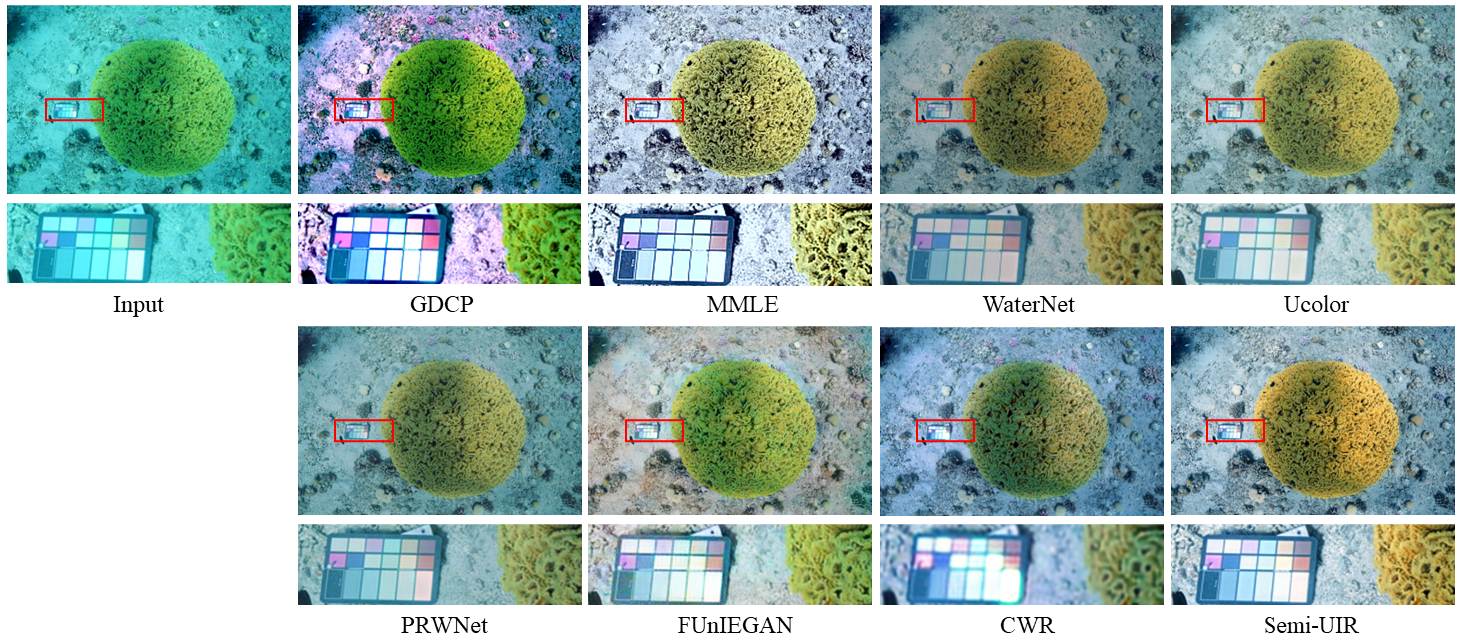
Results on full-reference datasets. The quantitative results on testS and testR are shown in Table 1. On testS, our method performs the best in PSNR, but slightly worse than Ucolor in terms of SSIM. One potential reason is that incorporating unlabeled real underwater images in training might emphasize the network to pay more attention to the real underwater scene. This can be confirmed by checking the quantitative results on testR. On testR, our method outperforms the other methods by a significant margin (outperforms the second best by 1.67dB in PSNR). In addition to the quantitative results, qualitative results are shown in Fig. 6. Our results are visually pleasant, while the compared methods suffer from color cast and over-enhancement.
| Method | UIQM (higher, better) | UCIQE (higher, better) | MUSIQ (higher, better) | |||||||||
|---|---|---|---|---|---|---|---|---|---|---|---|---|
| UIEB | EUVP | RUIE | Seathru | UIEB | EUVP | RUIE | Seathru | UIEB | EUVP | RUIE | Seathru | |
| Input | 3.066 | 4.729 | 3.948 | 5.925 | 0.509 | 0.517 | 0.490 | 0.537 | 41.70 | 42.73 | 33.53 | 60.25 |
| GDCPpeng2018gdcp | 3.401 | 4.738 | 4.509 | 5.343 | 0.564 | 0.599 | 0.565 | 0.590 | 40.07 | 42.49 | 34.63 | 60.54 |
| MMLEMMLE | 4.283 | 4.723 | 4.967 | 5.555 | 0.578 | 0.596 | 0.571 | 0.620 | 40.33 | 47.55 | 36.80 | 66.16 |
| WaterNetUIEBD | 4.118 | 5.317 | 4.568 | 6.829 | 0.572 | 0.595 | 0.572 | 0.610 | 40.32 | 43.07 | 32.23 | 64.38 |
| Ucolorucolor | 3.894 | 5.286 | 4.426 | 6.752 | 0.542 | 0.566 | 0.534 | 0.594 | 40.08 | 41.81 | 33.66 | 64.44 |
| PRWNetprwnet | 4.371 | 5.330 | 4.395 | 6.778 | 0.518 | 0.543 | 0.518 | 0.572 | 40.30 | 43.52 | 33.12 | 62.82 |
| FGANEUVP-FUnieGan | 4.315 | 4.469 | 4.519 | 4.853 | 0.541 | 0.561 | 0.527 | 0.564 | 40.95 | 43.36 | 34.48 | 64.25 |
| CWRcwr | 4.133 | 5.152 | 4.469 | 6.067 | 0.587 | 0.596 | 0.565 | 0.624 | 38.46 | 41.46 | 31.25 | 64.21 |
| Semi-UIR | 4.598 | 5.291 | 4.671 | 6.846 | 0.587 | 0.593 | 0.557 | 0.632 | 43.77 | 51.66 | 37.87 | 66.61 |

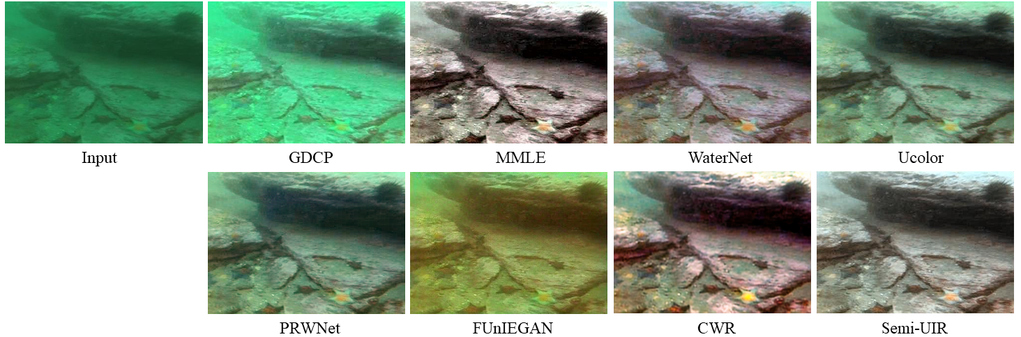
Results on non-reference datasets. The quantitative results on UIEB, EUVP, RUIE and Seathru are shown in Table 2. By quickly checking throughout the table, we can observed that our method significantly outperform the compared method in MUSIQ. Besides, we also achieve competitive performance in terms of UIQM and UCIQE. However, as is noted inberman2020underwater; UIEBD; guo2023uranker, UIQM and UCIQE might be biased to some characteristics and thus cannot accurately reflect the true visual quality of restored images. Similarly, the performance in MUSIQ is also for a reference. Therefore, the quantitative results might be insufficient to indicate the quality of restored underwater images due the underdeveloped NR-IQA metrics. We further show the qualitative results on the four benchmarks in Fig. 7. Compared with other methods, our approach can robustly restore various types of underwater images with natural color and rich details. Under the guidance of reliable pseudo labels and powerful contrastive regularization, our framework generalizes well on various underwater scenes.
4.4 Ablation Study
To analyze the effectiveness of Semi-UIR, we conduct ablation studies to reveal the influence of the key components in our method. They are presented as follows: (a) Sup-base: where we train the network AIM-Net without semi-supervised learning and unlabeled data. (b) Semi-base: Base semi-supervised training with consistency loss . (c) Semi-base+RB*: using reliable bank based on Semi-base without contrastive loss. (d) Semi-base+CL*: adding contrastive loss to Semi-base, without using reliable bank. (e) Semi-UIR: our proposed Semi-UIR.
The quantitative results of above methods are shown in Table 3. We can observe that our full solution performs best. In addition, by comparing Semi-base+RB* with Semi-base and Semi-UIR with Semi-base+CL*, it is easy to verify the effectiveness of incorporating the reliable bank.
Besides, the qualitative results are shown in Fig. 8, where special attention should be paid on Semi-base+CL* Semi-base+RB*. (1) In Semi-base+CL*, without the reliable positive samples, the contrastive loss pushes the network to produce extremely different results than the negative samples (inputs). However, this unfortunately results in over-enhancement. (2) On the contrary, in Semi-base+RB*, without the help of contrastive loss, the restored images still suffer from color distortion and are close to the degraded inputs. The two ablation studies verify the utility of the reliable bank and contrastive regularization.

| Method | MT | RB | CL | testR | EUVP | UIEB |
|---|---|---|---|---|---|---|
| Sup-base | 24.38 | 42.66 | 40.70 | |||
| Semi-base | 23.11 | 42.48 | 40.33 | |||
| Semi-base+RB* | 24.53 | 43.27 | 42.16 | |||
| Semi-base+CL* | 23.97 | 46.59 | 40.64 | |||
| Semi-UIR | 24.59 | 51.66 | 43.77 |
4.5 Breakdown of the Training
To further illustrate that the teacher’s outputs can be used to train student network, we here provide some intermediate results during training. The results are shown in Fig. 9. At the beginning of the training (10 epochs), the teacher’s prediction is much better than that of student. As the training processes, the student’s outputs and teacher’s outputs are improved simultaneously.

4.6 Influence of Non-reference Metric
We here conduct experiments to show the influence of using different NR-IQA approaches in building our reliable bank. We conclude in Sec. 3.4 that MUSIQ is the most reliable one. To further demonstrate the correctness of this selection, we here show the final performance of using NIMA, PAQ2PIQ and MUSIQ on the labeled dataset, i.e. testS and testR. Table 4 shows the results. It can be observed that we can achieve the best performance by using MUSIQ. It also shows that using PAQ2PIQ is better than using NIMA, which is consistent with their reliability shown in Fig. 4.
| Method | Reliability | PSNR | SSIM | ||
|---|---|---|---|---|---|
| testS | testR | testS | testR | ||
| NIMA | 41.05% | 23.01 | 23.88 | 0.815 | 0.888 |
| PAQ2PIQ | 82.11% | 23.08 | 24.28 | 0.818 | 0.893 |
| MUSIQ | 91.21% | 23.40 | 24.59 | 0.821 | 0.901 |
4.7 Influence of Data Augmentation
We finally show the influence of using different data augmentations in Table 5. By comparing the method using data augmentation with baseline, it is easy to conclude that adopting any of the data augmentations is beneficial. Besides, using a mixture of the three strategies achieves the best performance.
| Strategy | testR | UIEB | EUVP | RUIE | Seathru |
|---|---|---|---|---|---|
| Baseline | 0.880 | 40.12 | 46.06 | 31.14 | 64.71 |
| Color Jitter | 0.889 | 40.31 | 49.16 | 33.66 | 64.87 |
| Gaussian Blur | 0.896 | 41.23 | 49.27 | 36.88 | 64.88 |
| Gray Scale | 0.895 | 40.61 | 47.57 | 32.51 | 65.19 |
| All | 0.901 | 43.77 | 51.66 | 37.87 | 66.61 |
5 Conclusion
We propose an efficient semi-supervised underwater image restoration method named Semi-UIR. As demonstrated the ablation experiments, the superior performance of the proposed method over other SOTA algorithms can be attributed to reliable teacher-student consistency and contrastive regularization. The follow-up research can be carried out in two directions: 1) extend the semi-supervised framework to cover other restoration tasks, 2) optimize memory usage during training and improve performance via memory management.
References
- (1) Derya Akkaynak and Tali Treibitz. Sea-thru: A method for removing water from underwater images. In Proceedings of the IEEE/CVF conference on computer vision and pattern recognition, pages 1682–1691, 2019.
- (2) Codruta O Ancuti, Cosmin Ancuti, Christophe De Vleeschouwer, and Philippe Bekaert. Color balance and fusion for underwater image enhancement. IEEE Transactions on image processing, 27(1):379–393, 2017.
- (3) Dana Berman, Deborah Levy, Shai Avidan, and Tali Treibitz. Underwater single image color restoration using haze-lines and a new quantitative dataset. IEEE transactions on pattern analysis and machine intelligence, 43(8):2822–2837, 2020.
- (4) Stephan Brehm, Sebastian Scherer, and Rainer Lienhart. High-resolution dual-stage multi-level feature aggregation for single image and video deblurring. In Proceedings of the IEEE/CVF Conference on Computer Vision and Pattern Recognition Workshops, pages 458–459, 2020.
- (5) Ting Chen, Simon Kornblith, Mohammad Norouzi, and Geoffrey Hinton. A simple framework for contrastive learning of visual representations. In International conference on machine learning, pages 1597–1607. PMLR, 2020.
- (6) Zhixiang Chi, Xiao Shu, and Xiaolin Wu. Joint demosaicking and blind deblurring using deep convolutional neural network. In 2019 IEEE International Conference on Image Processing (ICIP), pages 2169–2173. IEEE, 2019.
- (7) Zhixiang Chi, Yang Wang, Yuanhao Yu, and Jin Tang. Test-time fast adaptation for dynamic scene deblurring via meta-auxiliary learning. In Proceedings of the IEEE/CVF Conference on Computer Vision and Pattern Recognition, pages 9137–9146, 2021.
- (8) Yimian Dai, Fabian Gieseke, Stefan Oehmcke, Yiquan Wu, and Kobus Barnard. Attentional feature fusion. In Proceedings of the IEEE/CVF Winter Conference on Applications of Computer Vision, pages 3560–3569, 2021.
- (9) Minghan Fu, Huan Liu, Yankun Yu, Jun Chen, and Keyan Wang. Dw-gan: A discrete wavelet transform gan for nonhomogeneous dehazing. In Proceedings of the IEEE/CVF Conference on Computer Vision and Pattern Recognition, pages 203–212, 2021.
- (10) Adrian Galdran, David Pardo, Artzai Picón, and Aitor Alvarez-Gila. Automatic red-channel underwater image restoration. Journal of Visual Communication and Image Representation, 26:132–145, 2015.
- (11) Jean-Bastien Grill, Florian Strub, Florent Altché, Corentin Tallec, Pierre Richemond, Elena Buchatskaya, Carl Doersch, Bernardo Avila Pires, Zhaohan Guo, Mohammad Gheshlaghi Azar, et al. Bootstrap your own latent-a new approach to self-supervised learning. Advances in neural information processing systems, 33:21271–21284, 2020.
- (12) Chunle Guo, Ruiqi Wu, Xin Jin, Linghao Han, Zhi Chai, Weidong Zhang, and Chongyi Li. Underwater ranker: Learn which is better and how to be better. In Proceedings of the AAAI Conference on Artificial Intelligence, 2023.
- (13) Junlin Han, Mehrdad Shoeiby, Tim Malthus, Elizabeth Botha, Janet Anstee, Saeed Anwar, Ran Wei, Mohammad Ali Armin, Hongdong Li, and Lars Petersson. Underwater image restoration via contrastive learning and a real-world dataset. Remote Sensing, 14(17):4297, 2022.
- (14) Kaiming He, Haoqi Fan, Yuxin Wu, Saining Xie, and Ross Girshick. Momentum contrast for unsupervised visual representation learning. In Proceedings of the IEEE/CVF conference on computer vision and pattern recognition, pages 9729–9738, 2020.
- (15) Byeongho Heo, Sanghyuk Chun, Seong Joon Oh, Dongyoon Han, Sangdoo Yun, Gyuwan Kim, Youngjung Uh, and Jung-Woo Ha. Adamp: Slowing down the slowdown for momentum optimizers on scale-invariant weights. In International Conference on Learning Representations (ICLR), 2021.
- (16) Muhammad Suzuri Hitam, Ezmahamrul Afreen Awalludin, Wan Nural Jawahir Hj Wan Yussof, and Zainuddin Bachok. Mixture contrast limited adaptive histogram equalization for underwater image enhancement. In 2013 International conference on computer applications technology (ICCAT), pages 1–5. IEEE, 2013.
- (17) Hanzhe Hu, Fangyun Wei, Han Hu, Qiwei Ye, Jinshi Cui, and Liwei Wang. Semi-supervised semantic segmentation via adaptive equalization learning. Advances in Neural Information Processing Systems, 34:22106–22118, 2021.
- (18) Fushuo Huo, Bingheng Li, and Xuegui Zhu. Efficient wavelet boost learning-based multi-stage progressive refinement network for underwater image enhancement. In Proceedings of the IEEE/CVF International Conference on Computer Vision, pages 1944–1952, 2021.
- (19) Md Jahidul Islam, Youya Xia, and Junaed Sattar. Fast underwater image enhancement for improved visual perception. IEEE Robotics and Automation Letters, 5(2):3227–3234, 2020.
- (20) Aupendu Kar, Sobhan Kanti Dhara, Debashis Sen, and Prabir Kumar Biswas. Zero-shot single image restoration through controlled perturbation of koschmieder’s model. In Proceedings of the IEEE/CVF Conference on Computer Vision and Pattern Recognition, pages 16205–16215, 2021.
- (21) Junjie Ke, Qifei Wang, Yilin Wang, Peyman Milanfar, and Feng Yang. Musiq: Multi-scale image quality transformer. In Proceedings of the IEEE/CVF International Conference on Computer Vision, pages 5148–5157, 2021.
- (22) Boyun Li, Xiao Liu, Peng Hu, Zhongqin Wu, Jiancheng Lv, and Xi Peng. All-in-one image restoration for unknown corruption. In Proceedings of the IEEE/CVF Conference on Computer Vision and Pattern Recognition, pages 17452–17462, 2022.
- (23) Chongyi Li, Saeed Anwar, Junhui Hou, Runmin Cong, Chunle Guo, and Wenqi Ren. Underwater image enhancement via medium transmission-guided multi-color space embedding. IEEE Transactions on Image Processing, 30:4985–5000, 2021.
- (24) Chongyi Li, Saeed Anwar, and Fatih Porikli. Underwater scene prior inspired deep underwater image and video enhancement. Pattern Recognition, 98:107038, 2020.
- (25) Chongyi Li, Chunle Guo, Wenqi Ren, Runmin Cong, Junhui Hou, Sam Kwong, and Dacheng Tao. An underwater image enhancement benchmark dataset and beyond. IEEE Transactions on Image Processing, 29:4376–4389, 2020.
- (26) Dong Liang, Ling Li, Mingqiang Wei, Shuo Yang, Liyan Zhang, Wenhan Yang, Yun Du, and Huiyu Zhou. Semantically contrastive learning for low-light image enhancement. In Proceedings of the AAAI Conference on Artificial Intelligence, volume 36, pages 1555–1563, 2022.
- (27) Huan Liu, Zijun Wu, Liangyan Li, Sadaf Salehkalaibar, Jun Chen, and Keyan Wang. Towards multi-domain single image dehazing via test-time training. In Proceedings of the IEEE/CVF Conference on Computer Vision and Pattern Recognition, pages 5831–5840, 2022.
- (28) Risheng Liu, Xin Fan, Ming Zhu, Minjun Hou, and Zhongxuan Luo. Real-world underwater enhancement: Challenges, benchmarks, and solutions under natural light. IEEE Transactions on Circuits and Systems for Video Technology, 30(12):4861–4875, 2020.
- (29) Yuyuan Liu, Yu Tian, Yuanhong Chen, Fengbei Liu, Vasileios Belagiannis, and Gustavo Carneiro. Perturbed and strict mean teachers for semi-supervised semantic segmentation. In Proceedings of the IEEE/CVF Conference on Computer Vision and Pattern Recognition, pages 4258–4267, 2022.
- (30) Ye Liu, Lei Zhu, Shunda Pei, Huazhu Fu, Jing Qin, Qing Zhang, Liang Wan, and Wei Feng. From synthetic to real: Image dehazing collaborating with unlabeled real data. In Proceedings of the 29th ACM International Conference on Multimedia, pages 50–58, 2021.
- (31) Cheng Ma, Yongming Rao, Jiwen Lu, and Jie Zhou. Structure-preserving image super-resolution. IEEE Transactions on Pattern Analysis and Machine Intelligence, 2021.
- (32) Yiqun Mei, Yuchen Fan, and Yuqian Zhou. Image super-resolution with non-local sparse attention. In Proceedings of the IEEE/CVF Conference on Computer Vision and Pattern Recognition, pages 3517–3526, 2021.
- (33) Anish Mittal, Anush Krishna Moorthy, and Alan Conrad Bovik. No-reference image quality assessment in the spatial domain. IEEE Transactions on image processing, 21(12):4695–4708, 2012.
- (34) Anish Mittal, Rajiv Soundararajan, and Alan C Bovik. Making a “completely blind” image quality analyzer. IEEE Signal processing letters, 20(3):209–212, 2012.
- (35) Takeru Miyato, Shin-ichi Maeda, Masanori Koyama, and Shin Ishii. Virtual adversarial training: a regularization method for supervised and semi-supervised learning. IEEE transactions on pattern analysis and machine intelligence, 41(8):1979–1993, 2018.
- (36) Karen Panetta, Chen Gao, and Sos Agaian. Human-visual-system-inspired underwater image quality measures. IEEE Journal of Oceanic Engineering, 41(3):541–551, 2015.
- (37) Adam Paszke, Sam Gross, Francisco Massa, Adam Lerer, James Bradbury, Gregory Chanan, Trevor Killeen, Zeming Lin, Natalia Gimelshein, Luca Antiga, et al. Pytorch: An imperative style, high-performance deep learning library. Advances in neural information processing systems, 32, 2019.
- (38) Yan-Tsung Peng, Keming Cao, and Pamela C Cosman. Generalization of the dark channel prior for single image restoration. IEEE Transactions on Image Processing, 27(6):2856–2868, 2018.
- (39) Boris T Polyak and Anatoli B Juditsky. Acceleration of stochastic approximation by averaging. SIAM journal on control and optimization, 30(4):838–855, 1992.
- (40) Olga Russakovsky, Jia Deng, Hao Su, Jonathan Krause, Sanjeev Satheesh, Sean Ma, Zhiheng Huang, Andrej Karpathy, Aditya Khosla, Michael Bernstein, Alexander C. Berg, and Li Fei-Fei. ImageNet Large Scale Visual Recognition Challenge. International Journal of Computer Vision (IJCV), 115(3):211–252, 2015.
- (41) Yoav Y Schechner and Nir Karpel. Clear underwater vision. In Proceedings of the 2004 IEEE Computer Society Conference on Computer Vision and Pattern Recognition, 2004. CVPR 2004., volume 1, pages I–I. IEEE, 2004.
- (42) Karen Simonyan and Andrew Zisserman. Very deep convolutional networks for large-scale image recognition. arXiv preprint arXiv:1409.1556, 2014.
- (43) Kihyuk Sohn, David Berthelot, Nicholas Carlini, Zizhao Zhang, Han Zhang, Colin A Raffel, Ekin Dogus Cubuk, Alexey Kurakin, and Chun-Liang Li. Fixmatch: Simplifying semi-supervised learning with consistency and confidence. Advances in neural information processing systems, 33:596–608, 2020.
- (44) Hossein Talebi and Peyman Milanfar. Nima: Neural image assessment. IEEE transactions on image processing, 27(8):3998–4011, 2018.
- (45) Antti Tarvainen and Harri Valpola. Mean teachers are better role models: Weight-averaged consistency targets improve semi-supervised deep learning results. Advances in neural information processing systems, 30, 2017.
- (46) Keyan Wang, Yan Hu, Jun Chen, Xianyun Wu, Xi Zhao, and Yunsong Li. Underwater image restoration based on a parallel convolutional neural network. Remote sensing, 11(13):1591, 2019.
- (47) Lin Wang and Kuk-Jin Yoon. Semi-supervised student-teacher learning for single image super-resolution. Pattern Recognition, 121:108206, 2022.
- (48) Xiaolong Wang, Ross Girshick, Abhinav Gupta, and Kaiming He. Non-local neural networks. In Proceedings of the IEEE conference on computer vision and pattern recognition, pages 7794–7803, 2018.
- (49) Xintao Wang, Ke Yu, Chao Dong, and Chen Change Loy. Recovering realistic texture in image super-resolution by deep spatial feature transform. In Proceedings of the IEEE conference on computer vision and pattern recognition, pages 606–615, 2018.
- (50) Yanbo Wang, Shaohui Lin, Yanyun Qu, Haiyan Wu, Zhizhong Zhang, Yuan Xie, and Angela Yao. Towards compact single image super-resolution via contrastive self-distillation. In Zhi-Hua Zhou, editor, Proceedings of the Thirtieth International Joint Conference on Artificial Intelligence, IJCAI-21, pages 1122–1128. International Joint Conferences on Artificial Intelligence Organization, 8 2021. Main Track.
- (51) Yuchao Wang, Haochen Wang, Yujun Shen, Jingjing Fei, Wei Li, Guoqiang Jin, Liwei Wu, Rui Zhao, and Xinyi Le. Semi-supervised semantic segmentation using unreliable pseudo-labels. In Proceedings of the IEEE/CVF Conference on Computer Vision and Pattern Recognition, pages 4248–4257, 2022.
- (52) Zhou Wang, Alan C Bovik, Hamid R Sheikh, and Eero P Simoncelli. Image quality assessment: from error visibility to structural similarity. IEEE transactions on image processing, 13(4):600–612, 2004.
- (53) Haiyan Wu, Yanyun Qu, Shaohui Lin, Jian Zhou, Ruizhi Qiao, Zhizhong Zhang, Yuan Xie, and Lizhuang Ma. Contrastive learning for compact single image dehazing. In Proceedings of the IEEE/CVF Conference on Computer Vision and Pattern Recognition, pages 10551–10560, 2021.
- (54) Miao Yang and Arcot Sowmya. An underwater color image quality evaluation metric. IEEE Transactions on Image Processing, 24(12):6062–6071, 2015.
- (55) Tian Ye, Sixiang Chen, Yun Liu, Yi Ye, Erkang Chen, and Yuche Li. Underwater light field retention: Neural rendering for underwater imaging. In Proceedings of the IEEE/CVF Conference on Computer Vision and Pattern Recognition (CVPR) Workshops, pages 488–497, June 2022.
- (56) Xiangyu Yin, Xiaohong Liu, and Huan Liu. Fmsnet: Underwater image restoration by learning from a synthesized dataset. In Artificial Neural Networks and Machine Learning–ICANN 2021: 30th International Conference on Artificial Neural Networks, Bratislava, Slovakia, September 14–17, 2021, Proceedings, Part III 30, pages 421–432. Springer, 2021.
- (57) Zhenqiang Ying, Haoran Niu, Praful Gupta, Dhruv Mahajan, Deepti Ghadiyaram, and Alan Bovik. From patches to pictures (paq-2-piq): Mapping the perceptual space of picture quality. In Proceedings of the IEEE/CVF Conference on Computer Vision and Pattern Recognition, pages 3575–3585, 2020.
- (58) Yankun Yu, Huan Liu, Minghan Fu, Jun Chen, Xiyao Wang, and Keyan Wang. A two-branch neural network for non-homogeneous dehazing via ensemble learning. In Proceedings of the IEEE/CVF conference on computer vision and pattern recognition, pages 193–202, 2021.
- (59) Syed Waqas Zamir, Aditya Arora, Salman Hameed Khan, Hayat Munawar, Fahad Shahbaz Khan, Ming-Hsuan Yang, and Ling Shao. Learning enriched features for fast image restoration and enhancement. IEEE Transactions on Pattern Analysis and Machine Intelligence, pages 1–1, 2022.
- (60) Shu Zhang, Ting Wang, Junyu Dong, and Hui Yu. Underwater image enhancement via extended multi-scale retinex. Neurocomputing, 245:1–9, 2017.
- (61) Weidong Zhang, Peixian Zhuang, Hai-Han Sun, Guohou Li, Sam Kwong, and Chongyi Li. Underwater image enhancement via minimal color loss and locally adaptive contrast enhancement. IEEE Transactions on Image Processing, 31:3997–4010, 2022.
- (62) Huabo Zhu, Xu Han, and Yourui Tao. Semi-supervised advancement of underwater visual quality. Measurement Science and Technology, 32(1):015404, 2020.
- (63) Xizhou Zhu, Han Hu, Stephen Lin, and Jifeng Dai. Deformable convnets v2: More deformable, better results. In Proceedings of the IEEE/CVF conference on computer vision and pattern recognition, pages 9308–9316, 2019.
- (64) Xiaojin Jerry Zhu. Semi-supervised learning literature survey. 2005.
Appendix A Supplementary Material
In the supplementary material, we first introduce the overall structure of our AIM-Net, details of validation set and loss functions, and then analyze the influence of the optimizer and NR-IQA metrics during training. Meanwhile, inherent advantage of Semi-UIR and additional experimental results on non-reference benchmarks are provided as well.
A.1 Details of the Network Structure
The goal of underwater image restoration is to conquer the problems such as low contrast, color distortion and blur. To this end, we propose an Asymmetric Illumination-aware Multi-scale Network (AIM-Net) to restore underwater images, as illustrated in Fig. 10. AIM-Net contains two important branches, namely illumination-aware restoration branch and gradient branch. The restoration branch adopts a multi-scale structure containing three parallel streams to exact precise spatial information and abundant contextual information in different scales. In addition, illumination prior is incorporated into the restoration branch to enhance the perception capability of color and light source. The simple gradient branch aims to recover high quality gradient map. The recovered gradient features are merged into the restoration branch to provide edge and structure prior.
The entire pipeline is as follows. The degraded image passes through a convolution layer to extract preliminary features. After that, the preliminary features are fed into the illumination-aware restoration branch to extract and integrate precise spatial information and contextual information. The illumination map is converted to illumination feature after a convolution layer. Then participates in the restoration branch via illumination guidance block (IGB) AirNet. On the other side, is fed into the gradient branch to restore fine gradient information. The gradient branch incorporates intermediate representations from the restoration branch because the intermediate representations carry rich structure information and are helpful for gradient map recovery. Later, attention feature fusion (AFF) block AFF fuses the fine features obtained by the two branches. Finally, the restored clear image and restored gradient map are both obtained after a convolution layer.
Illumination-aware Restoration Branch The task of the restoration branch is to reconstruct overall structure and color information of a degraded image. To complete the task, we introduce a parallel multi-scale structure incorporating illumination prior. The multi-scale structure can effectively integrate local details from different resolutions to maintain edge features and suppress halo artifacts wang2019underwater. Therefore, we adopt the structure of Multiscale Residual Block (MRB) MIRNetv2 as the backbone. MRB contains three parallel streams of different scales. Each stream utilizes residual contextual block (RCB) to distill useful spatial information and selective kernel feature fusion (SKFF) block to integrate contextual information. Based on the structure of MRB, we add several fundamental modules to further enhance feature extraction capability, including: multi-dilated-convolution block (MDB), IGB, non-local spatial attention (NLSA) block. Meanwhile, we replace the SKFF block with AFF block to better aggregate contextual information. These modules are described in detail as follows.
MDB works at the front of each stream to exact spatial features. It expands the receptive field via combing four dilated convolutions. Dilation rates are set as 1, 2, 3 and 4, consistent with dilated_conv. RCB MIRNetv2 distills useful contextual features by modeling and transforming the inter-channel dependencies via attention mechanism.
In the highest resolution stream, we introduce IGB between MDB and RCB to incorporate illumination prior. As is noted in UWNR, the illumination map reflects underwater light field information including ambient light and scene-dependent degradation that are essential for underwater image formation. As a result, we introduce the illumination map to help the network perceive color and light source information.

The illumination map is estimated in accordance with UWNR. IGB consists of a spatial feature transformation layer SFT and a deformable convolution deformable. In this way, our network can adapt to different color and light degradation types of underwater images.
To better integrate features from different scales, we replace SKFF module with AFF module. SKFF captures channel-wise dependencies via global-scale channel attention, whereas AFF squeezes local and global information into channel attention because local information is helpful to highlight local small targets AFF. The AFF module follows the RCB to aggregate local and global contextual features. Furthermore, we add NLSA module NLSA in the middle of the two lower resolution streams. NLSA models long-range feature correlations and enjoys robustness from sparse representation. Compared with the standard non-local attention NLA, it reduces computation expenses significantly.
With the help of the above well-designed modules, the network is able to extract fine feature representations. These feature representations are important for texture and color reconstruction.
Gradient Branch Image gradient map contains rich edge information and can guide the network to focus on local regions with sharp edges. As a result, we adopt the gradient map to enhance the edges of a restored image. Similar to spsr, the image gradient prior is introduced to promote the restoration of underwater images from two aspects: 1) a gradient branch to restore a high-quality gradient map and provide structural information for the restoration branch; 2) a supplementary gradient loss to constrain the second-order relationship of adjacent pixels, guiding the underwater image restoration to focus more on the geometry. The gradient branch first estimates a coarse gradient map of via gradient operation spsr, and then enhances the gradient map. Thanks to the intermediate representations from the restoration branch, the gradient branch can recover a fine gradient map with a very simple structure only including three convolution layers and two RCBs. Gradient loss is detailed in Eq. (9). Under these two types of guidance, the structure features can be better preserved, and the restoration results with sharper edges, higher perceptual quality and less geometric-inconsistent textures can be obtained.
In a word, AIM-net takes a degraded underwater image and its corresponding illumination map as input and outputs a restored clear image and a restored gradient map :
| (8) |
where represents the AIM-net parameterized by . AIM-Net has 1.675M parameters, and its inference speed is 33.3 FPS on the images with a resolution of 256× 256.
A.2 Details of Validation Set and Loss Functions
Our validation set, independent of testS and testR, contains 200 pairs of full reference underwater images from Anwar2019UWCNN; UIEBD with ratio 12:8.
The detailed perceptual loss and gradient penalty are as follows:
| (9) | ||||
where denotes perpetual loss based on pretrained VGG-16vgg network and denotes gradient loss. refer to ReLU1-2, ReLU2-2, and ReLU3-3 layers of the VGG-16 model. denotes clear ground truth. stands for the operation to extract a gradient mapspsr. constrains the restored gradient map of AIM-Net to approach the ground truth’s gradient map.
A.3 Influence of Optimizer and NR-IQA Metrics during Training
Table 6 shows the total training epochs required by Adam and AdamP to reach a similar accuracy. It can be observed that the training time required by Adam is longer than that by AdamP. Thus we choose AdamP as training optimizer.
| Optim | PSNR | SSIM | Epochs |
|---|---|---|---|
| Adam | 24.48 | 0.902 | 240 |
| AdamP | 24.59 | 0.901 | 200 |
To compare the efficiency of NR-IQA metrics, we additionally show the performance of adopting all seven NR-IQA metrics in Table 7. It is easy to check that using MUSIQ can achieve the best performance. Moreover, Fig. 11 presents some examples of pseudo labels (images in the reliable bank) selected by seven NR-IQA methods in the training process. It can be observed that MUSIQ can help select more visually pleasing pseudo labels (rightmost) over other metrics.
| NIQE | NIMA | UCIQE | BRISQUE | UIQM | PAQ2PIQ | MUSIQ | |
|---|---|---|---|---|---|---|---|
| Reliability | 13.45% | 41.05% | 48.16% | 48.69% | 76.87% | 82.11% | 91.21% |
| testS | 22.83/0.811 | 23.01/0.815 | 22.90/0.813 | 23.15/0.820 | 23.24/0.820 | 23.08/0.818 | 23.40/0.821 |
| testR | 22.98/0.887 | 23.88/0.888 | 23.64/0.890 | 24.00/0.900 | 23.80/0.897 | 24.28/0.893 | 24.59/0.901 |

A.4 Inherent Advantage of Semi-UIR
In order to verify the inherent advantage of our proposed semi-supervised restoration framework Semi-UIR, we replace the AIM-Net with 5-layer Unet used by FUnIE-GANEUVP-FUnieGan, and compare the performance using and not using Semi-UIR. Training details and datasets are unchanged. The quantitative results are shown in Table 8. It’s obvious that our semi-supervised framework Semi-UIR is beneficial to improve the generalizability of general model like Unet on real-world underwater benchmarks. It also demonstrates that Semi-UIR is extensible.
| Method | UIQM (higher, better) | UCIQE (higher, better) | MUSIQ (higher, better) | |||||||||
|---|---|---|---|---|---|---|---|---|---|---|---|---|
| UIEB | EUVP | RUIE | Seathru | UIEB | EUVP | RUIE | Seathru | UIEB | EUVP | RUIE | Seathru | |
| Unet-base | 4.215 | 4.442 | 4.529 | 4.970 | 0.585 | 0.583 | 0.554 | 0.603 | 39.33 | 43.87 | 31.17 | 62.92 |
| Unet-semi | 4.329 | 4.512 | 4.763 | 5.037 | 0.586 | 0.597 | 0.570 | 0.620 | 41.06 | 49.11 | 34.41 | 64.13 |
A.5 Additional Experimental Results on Non-reference Benchmark
In Fig. 12- 14, we present more results of our Semi-UIR on non-reference benchmarks Seathru seathru, RUIE liu2020real, UIEB UIEBD and EUVP EUVP-FUnieGan, and compare with the state-of-the-art methods including GDCP peng2018gdcp, MMLE MMLE, WaterNet UIEBD, Ucolor ucolor, FUnIE-GAN EUVP-FUnieGan, PRWNet prwnet and CWR cwr. Our proposed Semi-UIR outperforms other algorithms in restoring underwater images with rich details and natural color.