Endotactic and strongly endotactic networks with infinitely many positive steady states
Abstract
We show that there exists endotactic and strongly endotactic dynamical systems that are not weakly reversible and possess infinitely many steady states. We provide a few examples in two dimensions and an example in three dimensions that satisfy this property. In addition, we prove for some of these systems that there exist no weakly reversible mass-action systems that are dynamically equivalent to mass-action systems generated by these networks.
1 Introduction
Polynomial dynamical systems have profound applications in the study of ecology, epidemiology, and population dynamics. These dynamical systems are often of the form
| (1) |
where and . In particular, properties like extinction of species, persistence (property that no species goes extinct) and permanence (convergence to a compact set) are of paramount importance [13, 18, 10]. Many of these dynamical properties arise as a manifestation of the underlying structure of the reaction network. For example, it is conjectured that weakly reversible reaction networks (i.e., networks where every reaction is part of a directed cycle) are permanent. This is known as the Permanence conjecture [13]. Another important component in the analysis of dynamical systems is the study of steady states. We outline some important properties of steady states below.
Questions like the number of positive steady states, their stability and bifurcation are crucial to their analysis. In this paper, our focus is on the number of positive steady states. The analysis of steady states has a long history starting from the work on Deng et. al. [15], where they studied the existence and finiteness of steady states for weakly reversible networks. It has now been established by Boros [7] that for weakly reversible networks, there exists a positive steady state within each stoichiometric compatibility class. Further Boros, Craciun and Yu [8] have shown that there exists weakly reversible mass-action systems that possess infinitely many positive steady states; in particular they have constructed examples of weakly reversible mass-action systems where there is a curve of positive steady states. In this paper, we show that there exists examples of endotactic and strongly endotactic networks that possess a curve of positive steady states. The networks that appear in our construction are not weakly reversible; and in certain cases there exists no weakly reversible mass-action systems that are dynamically equivalent to the mass-action systems generated by these networks. In addition, we construct three dimensional endotactic networks that are not weakly reversible and possess infinitely many positive steady states.
In Section 2 we define reaction networks as graphs embedded in Euclidean space. In addition, we review some concepts from reaction network theory. In Section 3 we review certain properties about steady-states for weakly reversible and strongly endotactic networks. In Section 4 we define dynamically equivalent networks. In Section 5 we illustrate a set of simple operations on reaction networks that can be used to transform them to more complicated systems. In Section 6 we give examples of strongly endotactic and endotactic networks that are not weakly reversible but possess infinitely many steady states. In particular, we describe operations on a base unit network that eventually generate these endotactic and strongly endotactic networks. In Section 9 we review our results and chalk out directions for future research.
2 Reaction networks
A reaction network is a directed graph where reactions are represented by edges; reactant and product complexes are represented by vertices. Such graphs have been referred to as Euclidean embedded graphs(or E-graphs) [10, 11, 12, 9] in literature. We will denote this graph by , where is the set of vertices and is the set of edges. We will assume that and . We will denote the set of species by . A reaction will be denoted by the edge . We will denote by the set of source vertices. We define the following terms with respect to the reaction network :
- 1.
The stoichiometric subspace of a reaction network is the set . We will denote by the dimension of the stoichiometric subspace .
- 2.
The stoichiometric compatibility class of a point is the set .
- 3.
A set is called a linkage class if is a maximal connected component. We will denote the number of linkage classes in a network by .
- 4.
The deficiency of a network(denoted by is given by the formula: . Note that is an integer such that [20].
- 5.
A reaction network is weakly reversible if each reaction in the network is part of a directed cycle.
- 6.
- 7.
- 8.
A set of species is called a siphon if for every reaction the following holds true: if the complex does not contain any species from , then the complex also does not contain any species from .
- 9.
A set of species is said to be critical if there exists a point with if such that .
Figure 4 lists several examples of reaction networks that illustrates these properties.
The notions of endotactic and strongly endotactic network can be understood using the parallel sweep test [13, 18]. We state the test below for completeness.
Test 2.1 (Parallel sweep test for strongly endotactic networks).
Consider a reaction network . Let denote the stoichiometric subspace and denote the convex hull of the source vertices of . Choose a vector satisfying . Now sweep with a hyperplane perpendicular to towards . Let denote the hyperplane when it first touches the boundary of . Then the network is said to pass the parallel sweep for if the following conditions hold:
- 1.
For all reactions with source , we have and
- 2.
There exists at least one reaction with such that
We say that the network is strongly endotactic if it passes the parallel sweep testfor all . Otherwise, the network fails the parallel sweep test and is not strongly endotactic.

Test 2.2 (Parallel sweep test for endotactic networks).
Consider a reaction network . Let denote the stoichiometric subspace and denote the convex hull of the source vertices of . Choose a vector . Now sweep with a hyperplane perpendicular to towards . Let denote the hyperplane when it first touches the boundary of . We first verify if the following holds: for all reactions with source , we have . If no, then the network fails the parallel sweep test and is not endotactic. If yes, then we have two cases:
- 1.
If there exists at least one reaction with such that , then the network passes the parallel sweep test for .
- 2.
For all reactions with source , if we have , then we continue sweeping withe the hyperplane and repeat the steps above.
We say that the network is endotactic if it passes the parallel sweep test for all .
Note that weakly reversible reaction networks are endotactic. Strongly endotactic reaction networks are also endotactic. Further weakly reversible reaction networks consisting of a single linkage class are strongly endotactic. However, there exists endotactic reaction networks that are not weakly reversible; and endotactic networks that are not strongly endotactic.
Brunner et.al. [4] define extremally weakly reversible networks as those networks whose projections relative to the boundary of the convex hull of the source vertices are weakly reversible. They show that strongly endotactic networks in two dimensions are dynamically equivalent to some extremally weakly reversible network.
Reaction networks can be assigned a set of rate constants (one rate constant per reaction) which regulates the rate at which the species are produced or consumed. Given as assignment of rates, each reaction network can be linked to a set of dynamical system. In particular, if the dynamics is governed by mass-action kinetics [17, 25, 19, 26, 20, 1], then the rate equations are given by the following:
| (2) |
A point is called a steady state of 2 if . We will denote this mass-action dynamical system by . A mass-action system is said to be complex balanced if there exists such that the following is true for every vertex :
| (3) |
A lot of work hovers around inferring the dynamics of a reaction network from its underlying graphical structure. Such dynamical properties include persistence, permanence and global stability. The idea of persistence means that for any solution with , we have for all . A dynamical system is structurally persistent if the underlying reaction network does not possess critical siphons [5, 2]. Permanence is a stronger condition than persistence; in particular it implies that for every stoichiometric compatibility class , there exists a compact set such that the solution satisfies for large enough . A point is a global attractor if for any solution with , we have .
It is conjectured that weakly reversible reaction networks are permanent [13]. Further it is also conjectured that complex balanced systems have a globally attracting steady state within each stoichiometric compatibility class. This is known as the Global Attractor Conjecture. In recent years, there has been considerable progress in proving these conjectures. In particular, Craciun, Nazarov and Pantea [13] have proved that endotactic networks in two dimensions are permanent. This has been extended by Pantea [22] to networks with two dimensional stoichiometric subspace. Anderson [3] has shown that weakly reversible networks with a single linkage class are persistent. Gopalkrishnan, Miller and Shiu have shown that strongly endotactic networks are permanent. Angeli and Sontag [6] have shown that weakly reversible reversible networks that do not possess critical siphons are persistent. The entire proof of the Global Attractor Conjecture has been proposed in 2015 by Craciun [10].
3 Steady states
To understand the dynamics exhibited by reaction networks, it is important to analyze the behaviour of their steady states. In particular, phenomena like the existence of a unique steady state, or the the existence of multiple steady states or oscillations and bifurcations are of special interest. Proving the existence of positive steady states has received a lot of attention from the reaction network community. In particular, it is known that complex balanced dynamical systems have a unique steady state in each of their stoichiometric compatibility classes [21]. Further, these steady states are locally asymptotically stable. Boros [7] has shown that for weakly reversible networks, there exists a steady state within each stoichiometric compatibility class. Gopalkrishnan et.al. [18] have shown that strongly endotactic networks possess a positive steady state within each stoichiometric compatibility class.
In recent work, Craciun, Boros and Yu [8] have shown that there exists weakly reversible networks that possess infinitely many steady states. In particular, they have shown examples of weakly reversible networks that possess a curve of steady states. Our work extends this to show that there exists endotactic and strongly endotactic networks which are not weakly reversible, but possess a curve of steady states. Examples in Section 3 illustrate this point.
4 Dynamical Equivalence
The phenomenon of dynamical equivalence has been studied extensively in recent years. It has been also called macroequivalence by Horn and Jackson [21] and confoundability by Craciun and Pantea [14]. We formally define it below.
Definition 4.1.
Given dynamical systems and , we say that they are dynamically equivalent if the following holds for every
| (4) |
If two dynamical systems and are dynamically equivalent, we will denote this by .
5 Operations on Mass Action Systems
In this section, we describe different operations that we would be using on the mass-action systems in Section 6 such as: translation, scalar multiplication and addition.
5.1 Translation
For a mass-action system, when we multiply the right hand side of the dynamical system with by a monomial , it translates the system by a vector on the graph. For example consider the dynamical system given by:

| (5) | ||||
When we multiple the right-hand side of Equation 5 is multiplied by monomial , it translates the system by vector , and the dynamical system is given by:
Figure 5 represents the translation operation by a vector .
5.2 Scalar Multiplication
The scalar multiplication of the rate constant of the mass action system by a factor of give rise to two different behaviours depending upon the sign of the .
When , we modify the rate constants of the system by multiplying each of them with . For example, let us assume we have an initial mass action system as:
| (6) | ||||


We then multiply this dynamical system by on the right-hand side of Equation 6, we get the following dynamical system
When , we flip each reaction of the system along it’s source vertex and multiply to each rate coefficients by the absolute value of the . For example the initial system given by Equation 6 when multiplied by results in a dynamical system given by:
5.3 Addition and Simplification
Addition of two mass-action systems is equivalent to the following: take the union of all the reaction vectors of the two mass-action systems. The rate constants are added for the reaction vectors that are common to both the mass-action systems. For example consider the two mass-action systems:
| (7) | ||||
| (8) | ||||
We can also simplify the resultant mass-action system by combining similar monomials. This process will be called Simplification. For example, the addition of the mass-action systems given by Equations 7 and 8 is given by the following:


6 Strongly endotactic and endotactic reaction networks with infinitely many positive steady states
The goal of this section is to give a few examples of endotactic/strongly endotactic networks with infinitely many positive steady states. The idea of constructing these networks is similar to one described in [8]. For this process we start with a small unit, a simple endotactic/strongly endotactic network called the base unit. We then take multiple base units which are translated by multiplying with different scalar factors, which are combined and simplified to form a large reaction network that is endotactic/strongly endotactic but not weakly reversible.
Simplifying a reaction network refers to the process of reducing the differential equation to the minimum possible terms in such a way that the resultant reaction network is dynamically equivalent to the mass-action system generated by the original reaction network. The differential equation corresponding to the reaction network, comprises of two components
- •
Scalar Polynomial: It refers to common factor that represents the sum of the transformations of the base unit.
As remarked in [8], the key object here is called the Newton polytope [24], where the exponent corresponding to the negative monomial lies in the interior of the convex hull of exponents corresponding to the positive monomials. From [23], this implies that the sign of the polynomial near the boundary is positive. The polynomial evaluated at the point can be made negative, by choosing a sufficiently large negative coefficient corresponding to the negative monomial. This change in signs implies that the dynamical system has infinitely many positive steady states.
- •
Vector Polynomial: This part of the equation represents the dynamics corresponding to the base unit (which is a simple endotactic/strongly endotactic network) that we are using for construction of a complex reaction network. This base unit is then transformed by the scalar polynomial.
6.1 Example 1
We start with a base unit as given in Figure 8, where the rate constants corresponding to all reactions are set to 1. The network is not weakly reversible, has a deficiency of two and is endotactic, but not strongly endotactic. Further, the network possesses critical siphons implying that the dynamics generated by it is not structurally persistent. The properties mentioned above can be verified with the CoNtRol software [16].
Note that there exists no weakly reversible mass-action system that is dynamically equivalent to the mass-action system generated by the base unit. This base unit is then modified using certain transformations given in Figure 9. Combining these transformations, we obtain an endotactic mass action system as depicted in Figure 10. The dynamics of this system is given by:
6.1.1 Phase Plane Analysis
The positive steady states of the dynamical system are given by:


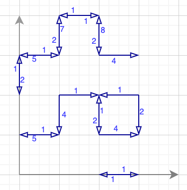
The curve of infinitely many positive steady states is the solution to the common term(scalar polynomial). The fixed point is the solution to the set vector polynomials. The phase portraits of the full system given in Figure 11 show a half-stable limit cycle, with a stable fixed point just outside the limit cycle. The phase portrait of the base unit also has a single stable fixed point at


We now describe the properties of the network corresponding to the full unit. The network is not weakly reversible, has a deficiency of eleven and is endotactic, but not strongly endotactic. Further, the network possesses critical siphons implying that the dynamics generated by it is not structurally persistent.
6.2 Example 2


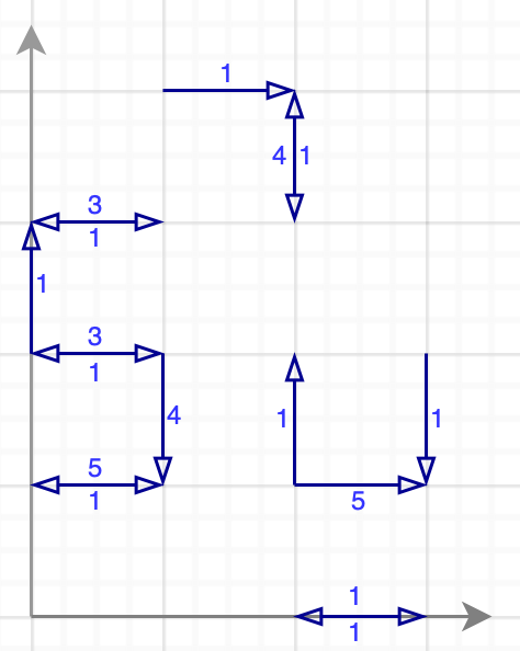
We start with a base unit given in Figure 12, where the rate constants corresponding to all reactions are all set to 1. This base unit is endotactic but not weakly reversible. The base unit is not weakly reversible, has a deficiency of two and is endotactic, but not strongly endotactic. Further, the network possesses critical siphons implying that the dynamics generated by it is not structurally persistent. The properties mentioned above can be verified with the CoNtRol software [16].
Further there exists no weakly reversible mass-action system that is dynamically equivalent to the mass-action system generated by the base unit. This base unit is then modified by using the transformations given in Figure 13. Combining these transformations we obtain an endotactic mass action system represented in Figure 14. Its dynamics is given by:
6.2.1 Phase Plane Analysis
The positive steady states of the dynamical system are given by:


The curve of the infinitely many steady states is the solution to the common term(scalar polynomial) and the point is the solution of the set of vector polynomials. The phase portrait of the full system given in Figure 15 shows a stable fixed point outside the curve of fixed points(which is a semi-stable limit cycle). The phase portrait of the base unit has a single stable fixed point at .
We now describe the properties of the network corresponding to the full unit. The network is not weakly reversible, has a deficiency of nine and is endotactic, but not strongly endotactic. Further, the network possesses critical siphons implying that the dynamics generated by it is not structurally persistent.
6.3 Example 3


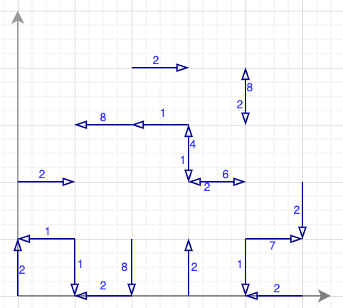
In this example, we start with a base unit given in Figure 16, where the rate constants corresponding to all reactions are set to 1. This base unit is strongly endotactic but not weakly reversible. The network has a deficiency of four and is strongly endotactic. Further, the network possesses no critical siphons implying that the dynamics generated by it is structurally persistent. The properties mentioned above can be verified with the CoNtRol software [16].
Further there exists no weakly reversible mass-action system that is dynamically equivalent to the mass-action system generated by the base unit. This base unit is then modified by using the transformations given in Figure 17. Combining these transformations we obtain a strongly endotactic mass action system depicted in Figure 18 The dynamics of the full unit is given by:
6.3.1 Phase Plane Analysis
The steady states of the system is given by:
The curve of infinite steady states is the solution to the common term(scalar polynomial) and the point is the solution for the set of vector polynomials. The phase portrait of the full system is given in Figure 19 show a unstable fixed point, surrounded by a stable limit cycle(which is a curve of infinite steady states.). The phase portrait of the base unit dynamical system have a single stable fixed point at (0.781, 1).


We now describe the properties of the network corresponding to the full unit. The network is not weakly reversible, has a deficiency of fifteen and is strongly endotactic. Further, the network possesses no critical siphons implying that the dynamics generated by it is structurally persistent.
7 Networks in three dimensions
The examples that we have analyzed so far are two dimensional. We now construct a three dimensional endotactic reaction network that is not weakly reversible but possesses a curve of infinitely many positive steady states.
7.1 Example
To come up with a base unit in three dimensions, we start with the two dimensional base unit given in Figure 12 and then combine it with a copy of itself transformed along the z-axis. To this system we add two reactions to connect the two planar vertices so that the reaction network looks like Figure 20.
The resultant network is not weakly reversible, has a deficiency of six and is endotactic, but not strongly endotactic. Further, the network possesses critical siphons implying that the dynamics generated by it is not structurally persistent. The properties mentioned above can be verified with the CoNtRol software.[16].
Note that there exists no weakly reversible mass-action system that is dynamically equivalent to the mass-action system generated by the base unit. The dynamics corresponding to the base unit is given by:

The base unit is then modified using certain transformations given in 21. The scalar polynomial for these transformations is given by:
Combining these transformations, we obtain the mass-action system depicted in figure 22(a).


7.1.1 Phase Plane Analysis
The steady states of the base system are given by:
where .
The dynamics generated by the base unit has infinitely many positive steady states which is given by a line of fixed points . The steady states of the full system is given by the set:
The full system gives us a curve of infinitely many steady states in , which is represented in Figure 22(b).
We now describe the properties of the network corresponding to the full unit. The network is not weakly reversible, has a deficiency of forty four and is endotactic, but not strongly endotactic. Further the network possesses critical siphons implying that the dynamics generated by it is not structurally persistent.


8 Appendix
8.1 Possible transformations of a reaction vector
In what follows, we list some transformations that can be done on a reaction vector and its rate constant so that the resultant system is dynamically equivalent to the original system.
8.1.1 Length transformation


This kind of transformation refers to the case where we modify the length of the reaction vector and its rate constant suitably, whilst keeping the direction of the reaction vector the same to ensure dynamical equivalence. Figure 23(a) gives an example of a scalar transformation of a reaction vector.
8.1.2 Diagonal decomposition
In this case, we take the reaction vector and decompose it into two reaction vectors, such that the original reaction vector bisects the two new vector. The rate constants of the new vectors are modified accordingly. Figure 23(b) gives an example of the this vector transformation.
8.2 Proof that there exists no weakly reversible mass-action systems that are dynamically equivalent to the mass-action systems generated by the full units in Examples 1 and 2


- 1.
Example 1: In Figure 24(a) we have the full unit given in Example 1. The boundary of the convex hull of the full unit is marked with a dotted red line. The problematic reaction is circled in green. There is no way which to return to the starting vertex, i.e. the point .
If we try to decompose the green reaction according to 8.1.2, the new vector that point outwards of the convex hull(on the right side), would again lead us to a vertex from where we cannot return.
If we try extending the reaction as we did in 8.1.1, the new reaction vector takes us to the point . From the point , we cannot go back to the upper part of the reaction network due to the reversible reaction vector between and Therefore, there exists no weakly reversible dynamical system that is dynamically equivalent to the mass-action system generated by the final system in Example 1.
- 2.
Example 2: In Figure 24(b) we have the full unit given in Example 2. The boundary of the convex hull of the full unit is marked with a dotted red line. The problematic reaction is circled in green. Arguing as in Example 1, there is no way to return to the starting vertex, i.e. the point . Therefore, there exists no weakly reversible dynamical system that is dynamically equivalent to the the mass-action system generated by the final system in Example 2.
9 Discussion
The study of steady states is crucial to the analysis of dynamical systems. In particular, questions about the existence and the number of steady states are of special importance. In particular, Boros [7] has established that for weakly reversible networks, there exists a positive steady state in every stoichiometric compatibility class. Gopalkrishnan, Miller ans Shiu have shown that strongly endotactic networks also possess at least positive steady state in every stoichiometric compatibility class. Boros, Craciun, and Yu [8] have shown that weakly reversible mass-action systems can possess infinitely many positive steady states. We extend this further to show that there exists endotactic and strongly endotactic networks that are not weakly reversible and possess infinitely many positive steady states. In addition, for the base and full units in Examples 1 and 2, there exists no weakly reversible systems that are dynamically equivalent to the mass-action systems generated by them.
This questions raises several intriguing questions for future work. For example,
- 1.
What is the minimal endotactic/strongly endotactic network that possesses infinitely many positive steady states? Here the phrase minimal could mean for e.g. the minimum number of reactions, or the minimum number of complexes or the minimum deficiency.
- 2.
Can one find conditions on the base unit, final unit and the scalar polynomial that ensures that there exists no weakly reversible systems that are dynamically equivalent to the mass-action systems generated by them?
- 3.
Can one find endotactic/strongly endotactic mass-action systems in higher dimensions (dimension greater than four) that are not weakly reversible and possess infinitely many positive steady states ?
- 4.
Is there a systematic way to construct such networks (i.e., can one design novel algorithms that can help us find such networks in practice?)
References
- [1] L. Adleman, M. Gopalkrishnan, M. Huang, P. Moisset, and D. Reishus, On the mathematics of the law of mass action, A Systems Theoretic Approach to Systems and Synthetic Biology I: Models and System Characterizations, Springer, 2014, pp. 3–46.
- [2] M Ali Al-Radhawi, D. Angeli, and E. Sontag, A computational framework for a lyapunov-enabled analysis of biochemical reaction networks, PLoS computational biology 16 (2020), no. 2, e1007681.
- [3] D. Anderson, A proof of the global attractor conjecture in the single linkage class case, SIAM J. Appl. Math. 71 (2011), no. 4, 1487–1508.
- [4] D. Anderson, J. Brunner, G. Craciun, and M. Johnston, On classes of reaction networks and their associated polynomial dynamical systems, J. Math. Chem. 58 (2020), no. 9, 1895–1925.
- [5] D. Angeli, P. De Leenheer, and E. Sontag, A petri net approach to persistence analysis in chemical reaction networks, Biology and Control Theory: Current Challenges (2007), 181–216.
- [6] , A petri net approach to the study of persistence in chemical reaction networks, Math. Biosci. 210 (2007), no. 2, 598–618.
- [7] B. Boros, Existence of positive steady states for weakly reversible mass-action systems, SIAM J. Math. Anal. 51 (2019), no. 1, 435–449.
- [8] B. Boros, G. Craciun, and P. Yu, Weakly reversible mass-action systems with infinitely many positive steady states, SIAM J. Appl. Math. 80 (2020), no. 4, 1936–1946.
- [9] C. Craciun, A. Deshpande, and J. Yeon, Quasi-toric differential inclusions, Discrete and Continuous Dynamical Systems - B 26 (2021), no. 5, 2343–2359.
- [10] G. Craciun, Toric differential inclusions and a proof of the global attractor conjecture, arXiv preprint arXiv:1501.02860 (2015).
- [11] , Polynomial dynamical systems, reaction networks, and toric differential inclusions, SIAM J. Appl. Algebra Geom. 3 (2019), no. 1, 87–106.
- [12] G. Craciun and A. Deshpande, Endotactic networks and toric differential inclusions, SIAM J. Appl. Dyn. Syst. 19 (2020), no. 3, 1798–1822.
- [13] G. Craciun, F. Nazarov, and C. Pantea, Persistence and permanence of mass-action and power-law dynamical systems, SIAM J. Appl. Math. 73 (2013), no. 1, 305–329.
- [14] G. Craciun and C. Pantea, Identifiability of chemical reaction networks, J. Math. Chem. 44 (2008), no. 1, 244–259.
- [15] J. Deng, C. Jones, M. Feinberg, and A. Nachman, On the steady states of weakly reversible chemical reaction networks, arXiv preprint arXiv:1111.2386 (2011).
- [16] P. Donnell, M. Banaji, A. Marginean, and C. Pantea, CoNtRol: an open source framework for the analysis of chemical reaction networks, Bioinformatics 30 (2014), no. 11, 1633–1634.
- [17] M. Feinberg, Lectures on chemical reaction networks, Notes of lectures given at the Mathematics Research Center, University of Wisconsin (1979), 49.
- [18] M. Gopalkrishnan, E. Miller, and A. Shiu, A geometric approach to the global attractor conjecture, SIAM J. Appl. Dyn. Syst. 13 (2014), no. 2, 758–797.
- [19] C. Guldberg and P. Waage, Studies Concerning Affinity, CM Forhandlinger: Videnskabs-Selskabet I Christiana 35 (1864), no. 1864, 1864.
- [20] J. Gunawardena, Chemical reaction network theory for in-silico biologists, Notes available for download at http://vcp. med. harvard. edu/papers/crnt. pdf (2003).
- [21] F. Horn and R. Jackson, General mass action kinetics, Arch. Ration. Mech. Anal. 47 (1972), no. 2, 81–116.
- [22] C. Pantea, On the persistence and global stability of mass-action systems, SIAM J. Math. Anal. 44 (2012), no. 3, 1636–1673.
- [23] C. Pantea, H. Koeppl, and G. Craciun, Global injectivity and multiple equilibria in uni- and bi-molecular reaction networks, Discrete Continuous Dyn. Syst. Ser. B. 17 (2012), no. 6.
- [24] B. Sturmfels, Grobner bases and convex polytopes, vol. 8, American Mathematical Soc., 1996.
- [25] E. Voit, H. Martens, and S. Omholt, 150 years of the mass action law, PLOS Comput. Biol. 11 (2015), no. 1, e1004012.
- [26] P. Yu and G. Craciun, Mathematical Analysis of Chemical Reaction Systems, Isr. J. Chem. 58 (2018), no. 6-7, 733–741.