Making Vision Transformers Efficient from A Token Sparsification View
Abstract
The quadratic computational complexity to the number of tokens limits the practical applications of Vision Transformers (ViTs). Several works propose to prune redundant tokens to achieve efficient ViTs. However, these methods generally suffer from (i) dramatic accuracy drops, (ii) application difficulty in the local vision transformer, and (iii) non-general-purpose networks for downstream tasks. In this work, we propose a novel Semantic Token ViT (STViT), for efficient global and local vision transformers, which can also be revised to serve as backbone for downstream tasks. The semantic tokens represent cluster centers, and they are initialized by pooling image tokens in space and recovered by attention, which can adaptively represent global or local semantic information. Due to the cluster properties, a few semantic tokens can attain the same effect as vast image tokens, for both global and local vision transformers. For instance, only 16 semantic tokens on DeiT-(Tiny,Small,Base) can achieve the same accuracy with more than 100% inference speed improvement and nearly 60% FLOPs reduction; on Swin-(Tiny,Small,Base), we can employ 16 semantic tokens in each window to further speed it up by around 20% with slight accuracy increase. Besides great success in image classification, we also extend our method to video recognition. In addition, we design a STViT-R(ecover) network to restore the detailed spatial information based on the STViT, making it work for downstream tasks, which is powerless for previous token sparsification methods. Experiments demonstrate that our method can achieve competitive results compared to the original networks in object detection and instance segmentation, with over 30% FLOPs reduction for backbone. Code is available at https://github.com/changsn/STViT-R.


1 Introduction
In contrast to standard Convolutional Neural Networks (CNNs) approaches which process images pixel-by-pixel, Vision Transformers (ViTs) dosovitskiy2020vit; touvron2021training; touvron2021going; liu2021swin; wu2021cvt treat an image as a sequence of patch/image tokens, and have shown promising performance in prevalent visual recognition scenarios. However, these superior performances do not come for free: the quadratic computational complexity to the number of image tokens limits their application in practice. Previous works song2021dynamic; zong2022self have illustrated the large amount of redundancy in the image tokens and also shown the effect of filtering out unimportant tokens normally according to predefined scoring mechanism. However, these methods face the following challenges. Firstly, the predefined scoring mechanisms for filtering are generally imprecise. In Figure 1, on the left we visualize the class token values in different layers which are commonly used to score the token importance xu2022evovit; fayyaz2021ats; liang2022evit. Different layers have different value distributions, thus using these imprecise scores for filtering would lead to unsatisfactory performance. For example, EViT liang2022evit has an accuracy drop of 1.3% when saving 50% FLOPs on DeiT-S touvron2021training. Secondly, the remaining tokens do not distribute evenly in space any more, making them hard to work in local vision transformers11 1 In this paper, we define the vision transformer with global self-attention (like DeiT) as global vision transformer and the vision transformer with local self-attention (like Swin) as local vision transformer.. Finally, large-scale token pruning tremendously damages the spatial structure and positional information, and causes difficulties when applied to downstream tasks, which they do not propose a solution to deal with.
To solve these problems, we propose Semantic Token ViT (STViT), for efficient global and local vision transformers, which also can be revised to serve as backbone for downstream tasks. The proposed approach is based on the following observations: (i) unlike local CNNs which learn spatial structure of images, vision transformer discretizes feature map as tokens for global feature exploration, relieving the requirements for maintaining the whole image structure and information; (ii) discrete tokens are more beneficial for optimization wang2021scaled; (iii) in Figure 1, on the right shows the attention maps in different transformer layers, and there are only several vertical lines in the deep layers, which means that only a few tokens with global semantic information matter. Thus, we argue that it is not necessary to maintain massive structured tokens for ViTs, especially in the deep layers. Employing a few discrete tokens with high-level semantic information can potentially achieve both high performance and efficiency.
In STViT, the semantic tokens represent the cluster centers, and the number of them is far less than the original image tokens, significantly reducing the computational cost. Inspired by the fact that multi-head attention can conduct the cluster center recovery (Appendix 6.6), we only employ the off-the-shelf self-attention to generate the semantic tokens. Specifically, the first few transformer layers are kept unchanged to obtain the image tokens with low-level features. The image tokens are then fed into our semantic token generation module (STGM) consisting of at least two transformer layers to generate semantic tokens. In each self-attention layer, the semantic tokens are input as queries, and the image tokens are fed as keys and values. The semantic tokens dynamically aggregate image tokens through the attention layers to recover cluster centers. In the first attention layer, the semantic tokens are initialized by an intra and inter-window spatial pooling which takes into account incorporating semantic information in each window and maximizing distance between adjacent windows. Thanks to this spatial initialization, the semantic tokens mainly incorporate local semantic information and achieve discrete and uniform distribution in space. In the following attention layer, besides further clustering, the semantic tokens are equipped with global cluster centers, and the network can adaptively select partial semantic tokens to focus on global semantic information. After the STGM, the original image tokens are discarded, and only semantic tokens are kept for the subsequent transformer layers. Because the generation of semantic tokens is flexible and space-aware, our method can be plugged into both global and local vision transformers. The semantic tokens can be produced in each window for the local vision transformer.
Another property of STViT is its capability to serve as a backbone for downstream tasks, such as object detection and instance segmentation. Discussions have been missing in all previous methods xu2022evovit; fayyaz2021ats; liang2022evit; ryoo2021tokenlearner; zong2022self about how to use them in downstream task under the massive loss of spatial information during the token sparsification process, which actually seriously impedes the application of their method. Instead, we design a novel STViT-R network based on STViT where a recovery module and dumbbell unit are adopted to periodically restore the full resolution feature map while the intermediate transformer layers continue to use semantic tokens to save computation cost, making our method work in downstream task.
The effectiveness of the proposed method is validated via a comprehensive empirical study on image and video ViT models. Only 16 semantic tokens on DeiT-(Tiny, Small, Base) achieve nearly 50% inference time reduction without any accuracy degradation; on Swin-(Tiny, Small, Base), we also improve the inference throughput by nearly 20% with slight accuracy increase. Moreover, the proposed STViT-R achieves promising results on object detection and instance segmentation. To the best of our knowledge, this is one of first works to apply the token sparsification algorithm in local vision transformers, and use the ViTs as backbones in downstream tasks after large-scale token pruning. Our findings in ViTs uncover that maintaining the full-size feature map is unnecessary, and a few tokens with high-level semantic representations can achieve both high performance and efficiency. Thanks to its simplicity and general-purpose ability, our method can also serve as a new efficient ViT baseline architecture and a starting point for further research from the token sparsification perspective.
2 Related work
Vision transformers.
Vision Transformer (ViT) dosovitskiy2020vit first introduces a pure Transformer backbone for image classification. ViT variants further inspire the applications of transformer to various vision tasks beyond image/video classification Yuan_2021_ICCV; touvron2021training; Xu_2021_ICCV; wang2021pyramid; wu2021cvt; touvron2021going; jiang2021all; bertasius2021space; arnab2021vivit; zhang2022morphmlp, such as object detection carion2020end; zhu2020deformable; zheng2020end; dai2021up, semantic segmentation wang2021max; wang2021end; zheng2021rethinking, and self-supervised learningchen2021mocov3; caron2021emerging; li2021efficient. Vanilla transformers have high computational and memory costs because the multi-head self-attention has quadratic computational complexity to the number of image tokens. Recently, various efficient ViTs have been proposed to alleviate this issue. The existing methods mainly focus on reducing the complexity of self-attention or reducing the number of tokens. Swin Transformer liu2021swin adopts local self-attention, i.e., attending neighboring tokens within a constant window size, achieving a linear computational complexity in the self-attention with high performance. Many subsequent works dong2021cswin; yu2022boat; wang2021crossformer; yang2021focal; huang2021shuffle; zhou2021elsa; chu2021twins follow the local self-attention design to develop variants. Token sparsification rao2021dynamicvit; wang2021not; pan2021ia; ryoo2021tokenlearner; chen2021chasing; song2021dynamic; yin2022vit; meng2021adavit; fayyaz2021ats; xu2022evovit; zong2022self; tang2021patch; kong2021spvit; liang2022evit also attracts increasing attention.
Token sparsification.
Token sparsification methods can be mainly categorized into hard pruning rao2021dynamicvit; pan2021ia; chen2021chasing; song2021dynamic; yin2022vit; meng2021adavit; fayyaz2021ats; xu2022evovit; kong2021spvit; liang2022evit; tang2021patch and soft pruning ryoo2021tokenlearner; zong2022self. Hard pruning methods filter out some unimportant tokens according to a predefined scoring mechanism. DynamicViT rao2021dynamicvit, SPViT kong2021spvit, and AdaViT meng2021adavit introduce additional prediction networks to score the tokens. Evo-ViTxu2022evovit, ATS fayyaz2021ats, and EViT liang2022evit utilize the values of class tokens to evaluate the importance of tokens. However, it is difficult to achieve precise scoring as shown in the left of Figure 1. Therefore, they usually suffer from a significant accuracy drop. For instance, EViT liang2022evit has an accuracy drop of 1.3% when saving 50% FLOPs on DeiT-S. Soft pruning methods generate new tokens from image tokens by importing additional attention networks. TokenLearner ryoo2021tokenlearner also argue for a few tokens to replace image tokens. However, its price is a 1.8% accuracy drop when reducing 44% FLOPs, which is far inferior to concurrent works. Besides performance degradation, previous methods also have the following disadvantages. First, whether or how to extend the methods to local vision transformers remains unexplored. Second, it has not been discussed about how to serve the downstream tasks like object detection and instance segmentation after the tokens are pruned.
In our method, we apply the off-the-shelf transformer layers to reduce token number. ma2021luna; jaegle2021perceiver; bai2021visual; zhang2019latentgnn; li2019expectation; chen2019graph adopt similar approaches to achieve efficient non-local relationships. Our method is different from them as below: (i) our method extracts local semantic information instead of non-local relationships; (ii) the semantic tokens are a few cluster centers, which can replace the massive image tokens to achieve image classification; (iii) our method specializes in pruning tokens.
3 Method
The proposed STViT is presented in this section, which aims to construct an efficient and high-performance ViT. STViT is first introduced in Section 3.1, followed by how to apply STViT in the local vision transformer in Section 3.2. Based on STViT, STViT-R is developed to restore the spatial resolution for downstream tasks in Section 3.3.
3.1 STViT
Overall architecture.
An overview of STViT architecture is presented in Figure 2(a). The patch embedding layer and shallow transformer layers are kept unchanged as a base module in our method. The base module copes with all the image tokens to extract low-level features, where is the number of image tokens and is the number of channels. The image tokens are fed into the semantic token generation module (STGM) to generate semantic tokens . After the STGM, the image tokens can be discarded, and only semantic tokens with high-level semantic information are used in all the subsequent transformers. Due to , our method can significantly reduce the computational cost.


Semantic token generation module (STGM).
The whole image is represented by a few tokens with high-level semantic information through clustering. Inspired by the fact that self-attention can conduct cluster center recovery (Appendix 6.6), we adopt the off-the-shelf self-attention layers to produce the semantic tokens. The STGM consists of at least two transformer layers.
The initial cluster centers are generated by an spatial pooling which pools the image tokens into fixed tokens, with . is generally set as . The spatial pooling can be achieved by a non-parameterized adaptive spatial pooling or a super lightweight network with higher performance, intra and inter-window spatial pooling. The intentions of spatial pooling initialization are three folds. First, the initial cluster centers can distribute uniformly in space, making the generated semantic tokens more discrete and preventing the semantic tokens from collapsing to one point in the following layers. Second, the semantic tokens can be forced to represent more local and distinguished features. Finally, the representation of semantic tokens is associated with the specific spatial locations, which is the basis to allow our method to be applied in local self-attention and downstream tasks. The initial cluster centers then dynamically integrate the image tokens according to semantic information by attention mechanism. In the first transformer layer, the processing of the generation of semantic tokens can be written as
| (1) |
where and are short for multi-head attention layer and feed-forward network, respectively, and the triplet input of are queries, keys, and values in turn. All the norm layers are omitted in all the equations for brevity. The initial cluster centers are produced in a window by an adaptive spatial pooling layer or an intra and inter-window spatial pooling, while the semantic tokens are generated from a global receptive field by a dynamic attention layer to ensure that they can extract high-level semantic representation. In order to further strengthen the clustering effect, we use the second transformer layer to repeat the clustering operation and guide the semantic tokens to extract global information. In this transformer layer, the semantic tokens are updated as:
| (2) |
where is the global cluster centers initialized by Gaussian noise and is a concatenation operation. The global cluster centers are responsible for global semantic information extraction like the class token. Although and are summed together as the queries, they can be decoupled in the attention computation as:
| (3) |
where and are the linear projection weights of queries and keys. We can see that and integrate the keys to generate and independently and just share a Softmax operation to produce the final attention map . Therefore, besides spatial semantic information, the semantic tokens also incorporate global semantic information with a negligible additional overhead. Though very similar, the global cluster centers are actually different from the learned positional encoding. We do not add the global cluster centers to keys. Moreover, it will be shown in the experiments that inserting the actual learned positional encoding will cause an accuracy drop. The number of transformer layers in STGM is flexible. More transformer layers can be associated for clustering. Two transformer layers are employed by default, i.e., is the output of the STGM. Note that the image tokens are not updated in the STGM.
Intra and inter-window spatial pooling.
Give feature map , we generate () initial cluster centers. We uniformly split the into windows with size and each window generates one initial cluster center. To represent abundant semantic information, we take into account intra and inter-window relations, i.e., integrating important tokens in the window and maximizing the distance among initial cluster centers in different windows. Specifically, we formulate an intra-window function to produce a mask, , which projects the input window from . The idea is to let the intra-window function adaptively select a combination of informative tokens in , which is implemented by
|
. |
(4) |
Then, we compute each integrated token from each window, and arrange by spatial structure to form the 2D tensor . We adopt an inter-window function to compute the inter-window relations and generate the offset, ,to revise the mask . The implementation of is similar to Eq. 4, except the mapping input from , where is the number of tokens in each window. For each window, the corresponding is sliced from and reshaped to . The is used to revise . The final initial cluster center is computed by
| (5) |
Our and are super lightweight and the introducing parameters can be negligible. For example, on DeiT-T, the parameters only increase by 0.05%.
3.2 STViT in local vision transformers.
Local self-attention has been widely used in current ViT models to balance efficiency and accuracy. As the generation of semantic tokens in STViT is flexible in space, it can be naturally applied in local self-attention. Suppose each local self-attention layer contains windows with size , we initialize cluster centers in each window by our intra and inter-window spatial pooling. The total number of semantic tokens would be . and are set as and by default separately. As a result, our method compresses more than 80% image tokens in local self-attention. In the STGM, although initial cluster centers are from windows, we use larger windows with size to obtain keys and values in Eq. 1 and Eq. 2 to mitigate the effect of limited window size. Other operations in STGM are kept the same as Section 3.1.
In the local ViT models, each local transformer layer is normally followed by a cross-window connection layer, such as a shift window transformer layer following a local transformer layer on Swin Transformer liu2021swin. In our method, the attention is computed within window in the local self-attention layer, and the cross-window connection can be achieved by computing self-attention in a larger-size (e.g., ) sliding window because of the rare number of tokens in each window. For the low-resolution input, our cross-window connection layer is equal to a global self-attention layer.
3.3 STViT for downstream tasks
Our method significantly reduces the computation cost by using a small number of semantic tokens, while its side effect is losing nearly all the detailed position information. High-level vision tasks, such as object detection and instance segmentation, are difficult to be executed on this extremely incomplete feature map. This issue also exists in previous works, which hinders the application of token sparsification methods. To solve this issue, we design a STViT-R network based on STViT to restore the original spatial resolution from the semantic tokens.
Our STViT-R shown in Figure 2(b) has two modifications compared with STViT. First, we adopt a recovery module to restore the spatial resolution from semantic tokens; second, we regroup the transformer layers and construct dumbbell units composed of our STViT-R.
Recovery module.
In the recovery module, only the self-attention layer is employed to restore the spatial resolution without any additional networks. The image tokens and semantic tokens are partitioned as windows of size and , respectively. The image tokens in each window aggregate the semantic tokens in the corresponding window, which is represented as:
| (6) |
This is a reverse operation of the generation of semantic tokens, using high-level semantic information to boost the image tokens.
Dumbbell unit.
The transformer layers are regrouped into multiple dumbbell units in our STViT-R. Each dumbbell unit consists of four parts. The transformers in the first part are responsible for coping with image tokens; the second part is the semantic token generation module; the transformer layers in the third part deal with semantic tokens; the last part is the recovery module. Take the application on Swin-S (STViT-R-Swin-S) as an example. One, two, two and one transformer layers are allocated for these four parts, respectively. In total, each dumbbell unit is composed of 6 transformer layers. We concatenate three dumbbell units in Stage 3 of Swin-S. In each dumbbell unit, the intermediate transformer layers process semantic tokens with high-level semantic information to save computational cost, and the complete spatial resolution is recovered at the end. By repeating multiple dumbbell units, the detailed spatial information will be preserved by the network, which can not only enhance the classification but also serve downstream tasks.
4 Experiments
STViT will first be applied in two representative ViT models, DeiT touvron2021training and Swin liu2021swin for image classification and video recognition. To validate that our method is effective in downstream tasks, STViT-R is then performed on object detection and instance segmentation tasks.
4.1 Image classification
Settings.
For image classification, all the models are trained on the ImageNet deng2009imagenet with 1.28M training images and 50K validation images from 1,000 classes. By default, the semantic token generation module (STGM) employs the and transformer layers of DeiT (with 12 layers in total), employs the and transformer layers of Stage 3 of Swin-T (with 12 layers in total), and employs the and transformer layers of Stage 3 of Swin-S and Swin-B (with 24 layers in total). The image resolution in training and inference is unless otherwise specified. The batch size is 1,024. All the models are trained from scratch for 300 epochs, and the augmentation and regularization strategies follow the original papers of DeiT and Swin. No knowledge distillation algorithms are used in our experiments. The classification is performed by applying a global average pooling layer on the output tokens of the last transformer layer, followed by a linear classifier. In evaluation, the top-1 accuracy using a single crop is reported. The FLOPs computations of this paper are measured by Fvcore22 2 https://github.com/facebookresearch/fvcore. Throughput is measured with the batch size of 128 on a V100 GPU.
On Swin liu2021swin, the semantic tokens are generated in Stage 3, and they are not downsampled in Stage 4 due to rare semantic tokens. The patch merging layer between Stage 3 and Stage 4 is replaced with a simple linear layer to double the number of channels. is set as 10 and 14 for two transformer layers of STGM.
| Model | Metrics | Base | No. of semantic tokens | |||
|---|---|---|---|---|---|---|
| 16 | 36 | 64 | 100 | |||
| STViT-DeiT-T | Top-1 Acc(%) | 72.2 | 72.2(+0.0%) | 72.7(+0.5) | 73.0(+0.8) | 73.2(+1.0) |
| FLOPs(G) | 1.26 | 0.53(-58%) | 0.60(-52%) | 0.71(-44%) | 0.86(-32%) | |
| Throughput(img/s) | 2752 | 5511(+101%) | 4769(+74%) | 4214(+53%) | 3551(+29%) | |
| STViT-DeiT-S | Top-1 Acc(%) | 79.8 | 79.8(+0.0) | 80.1(+0.3) | 80.5(+0.7) | 80.6(+0.8) |
| FLOPs(G) | 4.58 | 1.91(-58%) | 2.20(-52%) | 2.62(-43%) | 3.16(-31%) | |
| Throughput(img/s) | 1408 | 2891(+105%) | 2542(+80%) | 2229(+58%) | 1837(+30%) | |
| STViT-DeiT-B | Top-1 Acc(%) | 81.8 | 81.8(+0.0) | 82.2(+0.4) | 82.6(+0.8) | 82.7(+0.9) |
| FLOPs(G) | 17.58 | 7.31(-58%) | 8.44(-52%) | 10.04(-43%) | 12.13(-31%) | |
| Throughput(img/s) | 626 | 1308(+110%) | 1150(+85%) | 1087(+61%) | 826(+33%) | |
| Model | Metrics | Base | Move | No. of semantic tokens | ||
|---|---|---|---|---|---|---|
| STGM | 4 | 9 | 16 | |||
| STViT-Swin-T | Top-1 Acc(%) | 81.3 | 81.0(-0.3%) | 80.8(-0.5) | 81.5(+0.2) | 81.8(+0.5%) |
| FLOPs(G) | 4.5 | 3.14(-30%) | 2.99(-34%) | 3.43(-24%) | 4.06(-10%) | |
| Throughput(img/s) | 878 | 1124(+29%) | 1128(+29%) | 1061(+22%) | 1008(+15%) | |
| STViT-Swin-S | Top-1 Acc(%) | 83.0 | 82.8(-0.2%) | 82.4(-0.6%) | 83.0(-0.0) | 83.1(+0.1%) |
| FLOPs(G) | 8.7 | 5.95(-32%) | 5.95(-32%) | 6.53(-25%) | 7.36(-15%) | |
| Throughput(img/s) | 551 | 739(+35%) | 732(+34%) | 691(+26%) | 657(+20%) | |
| STViT-Swin-B | Top-1 Acc(%) | 83.5 | 83.2(-0.3%) | 83.0(-0.5) | 83.4(-0.1) | 83.7(+0.2%) |
| FLOPs(G) | 15.4 | 10.48(-32%) | 10.48(-32%) | 11.51(-25%) | 12.97(-16%) | |
| Throughput(img/s) | 415 | 558(+35%) | 551(+33%) | 521(+26%) | 489(+19%) | |
Results.
One of the advantages of our method is that it can be applied to both global and local vision transformers to reduce computational complexity. Our main results on DeiT and Swin are summarized in Table 1 and Table 2, respectively. The results of LV-ViT jiang2021all are illustrated in Appendix 6.2 due to limited space. We report the top-1 accuracy, FLOPs, and the throughput under different numbers of semantic tokens. On DeiT, the models with 16 semantic tokens achieve the same accuracy as the DeiT models with 196 tokens and save nearly 60% FLOPs on DeiT-T, DeiT-S, and DeiT-B. With more semantic tokens, the accuracy can consistently outperform the base models. For instance, STViT-DeiT-B with 36 semantic tokens surpasses DeiT-B by 0.4% accuracy with 52% FLOPs reduction.
The local vision transformer like Swin is already an efficient architecture compared to the global vision transformer, so the reduction of FLOPs on Swin models are smaller than on DeiT models. When 9 semantic tokens are used in each window, STViT-Swin models can reduce 25% FLOPs with negligible accuracy loss on all the model sizes. If the number of tokens is reduced to 4 in each window (16 in total), a significant accuracy drop will occur, which indicates that local vision transformers need more semantic tokens than global vision transformers. We can move the STGM towards shallow layers to attain a better complexity/accuracy trade-off. In Table 2, STGM is moved by one transformer layer on STViT-Swin-T and by two layers on STViT-Swin-S and STViT-Swin-B to save over 30% FLOPs with only about 0.3% accuracy drops (column of “Move STGM”).
STViT-R equipped with recovery modules is designed for downstream tasks, while it also can perform image classification. The corresponding results are reported in Table 3. On both Swin-S and Swin-B, STViT-R can save 33% FLOPs with 0.3% accuracy drop. The hyper-parameters we used in STGM are as same as STViT-Swin.
These results demonstrate that our method achieves both effectiveness and efficiency by employing a few semantic tokens to replace original image tokens. Our method reveals that constructing the tokens with high-level semantic representation is more important than maintaining structured tokens in ViTs. As reflected by the throughput, our method does not have overhead of memory or deployment. Compared to the total parameters, the additional parameters introduced by intra and inter-window spatial pooling is negligible(less than 0.05%), so we do not show them.
| Model | Top-1 Acc(%) | FLOPs(G) | Throughput |
|---|---|---|---|
| STViT-R-Swin-S | 82.7(-0.3) | 5.83(-33%) | 717(+30%) |
| STViT-R-Swin-B | 83.2(-0.3) | 10.26(-33%) | 539(+30%) |
| Model | Top-1 Acc | FLOPs(G) | |
| DeiT-S | |||
| DynamicViT rao2021dynamicvit | 79.3 | 2.9(-37%) | -0.5 |
| IA-RED2 pan2021ia | 79.1 | 3.2(-30%) | -0.7 |
| PS-ViT tang2021patch | 79.4 | 2.6(-43%) | -0.4 |
| TokenLearner ryoo2021tokenlearner | 76.1 | 1.9(-44%) | -1.8 |
| DGE* song2021dynamic | 79.7 | 3.1 (-49%) | -0.6 |
| A-ViT* yin2022vit | 78.6 | 3.6 (-39%) | -0.3 |
| Evo-ViT xu2022evovit | 79.4 | 3.0(-35%) | -0.4 |
| EViT liang2022evit | 78.5 | 2.3(-50%) | -1.3 |
| STViT(Ours) | 79.8 | 1.91(-58%) | -0.0 |
| DeiT-B | |||
| IA-RED2 pan2021ia | 80.3 | 11.8(-33%) | -1.5 |
| DynamicViT rao2021dynamicvit | 81.3 | 11.2(-36%) | -0.5 |
| PS-ViT tang2021patch | 81.5 | 9.8(-44%) | -0.3 |
| TokenLearner* ryoo2021tokenlearner | 83.7 | 28.7(-48%) | -1.1 |
| Evo-ViT xu2022evovit | 81.3 | 10.2(-33%) | -0.5 |
| EViT liang2022evit | 80.0 | 8.7(-51%) | -1.8 |
| STViT(Ours) | 81.8 | 7.31(-58%) | -0.0 |
| APb | AP | AP | AP | APm | AP | AP | AP | FLOPs(G) | |
|---|---|---|---|---|---|---|---|---|---|
| Swin-S | 51.8 | 70.4 | 56.3 | 35.2 | 44.7 | 67.9 | 48.5 | 28.8 | 194 |
| STViT-R-Swin-S | 51.8 | 70.6 | 56.1 | 36.7 | 44.7 | 67.8 | 48.6 | 29.0 | 134(-31%) |
| Swin-B | 51.9 | 70.9 | 56.5 | 35.4 | 45.0 | 68.4 | 48.7 | 28.9 | 343 |
| STViT-R-Swin-B | 52.2 | 70.8 | 56.8 | 36.5 | 45.2 | 68.3 | 49.1 | 29.5 | 233(-32%) |
Comparisons with existing token sparsification methods.
In Table 4, we compare STViT with the state-of-the-art token sparsification methods on DeiT-S and DeiT-B. Due to different base models used by different methods, we adopt accuracy difference between each model and its base model to evaluate them for fair. Results indicate that our method achieves the lowest accuracy drop with the highest FLOPs reduction, outperforming all the state-of-the-art methods in both accuracy and efficiency significantly.
4.2 Video recognition
Setting.
For video recognition, we apply our STViT to Video Swin liu2022video. All the models are pre-trained on ImageNet-1K and trained on Kinetics-400 carreira2017quo. We generate semantic tokens from each frame as illustrated in Section 3.2. The initialization from pre-trained models and other implementation details are as same as Video Swin liu2022video.
Results.
The results are presented in Table 6. On Swin-T and Swin-S, STViT-Swin can save about 27% FLOPs with 0.3% accuracy drop, which shows that our method works on video recognition.
4.3 Applications in object detection and instance segmentation
Settings.
Experiments of object detection and instance segmentation are conducted on COCO 2017 lin2014microsoft. We evaluate STViT-R with Swin in Cascade Mask R-CNN cai2018cascade; he2017mask detection frameworks. The is set to . The backbone models are pre-trained on ImageNet-1K and the pre-trained results are presented in Table 3. All the other settings follow Swin liu2021swin.
Comparison to Swin Transformer.
The performance of STViT-R-Swin using the Cascade Mask R-CNN framework with schedule is shown in Table 5. Our method achieves better performance with more than 30% FLOPs reduction for backbone on bath object detection and instance segmentation. This validates that the recovery module and dumbbell unit can restore detailed spatial information, and the global context information integrated from the semantic tokens significantly benefits object detection. Ignoring spatial structure in the intermediate layers does not affect the object detection task, which is a meaningful fact to help design efficient object detection frameworks. Another interesting finding is that our method has a remarkable improvement for small object detection which is a challenging problem in the detection community. For instance, our STViT-R-Swin-S outperforms Swin-S by 1.5% on .
| Model | Top-1 Acc(%) | FLOPs(G) | Speed |
|---|---|---|---|
| Swin-T | 78.8 | 88 | 779 |
| STViT-Swin-T | 78.5(-0.3) | 64.4(-27%) | 975(+25%) |
| Swin-S | 80.6 | 166 | 456 |
| STViT-Swin-S | 80.3(-0.3) | 120.5(-27%) | 572(+25%) |
| Spatial | Global | Learned | Top-1 Acc(%) |
| ✓ | 79.4 | ||
| ✓ | 78.7 | ||
| ✓ | ✓ | 79.8 | |
| ✓ | ✓ | 79.7 |
| No. of transformers | 2 | 3 | 4 |
|---|---|---|---|
| Top-1 Acc(%) | 79.8 | 79.5 | 79.6 |
| FLOPs(G) | 1.91 | 1.97 | 2.03 |
| STViT-R | w/o DU | Reusing ST | |
|---|---|---|---|
| APb | 51.8 | 51.4 | 51.6 |
| APm | 44.7 | 44.4 | 44.5 |
4.4 Ablation study
All the following ablation experiments of STViT and STViT-R are conducted on the DeiT-S and Swin-S, respectively.
Initialization analysis.
The semantic tokens are the cluster centers recovered by attention layers. The initialization of cluster centers induces the representation of semantic tokens. Spatial and global initialization are adopted in Section 3.1 to guide the semantic tokens to integrate local and global semantic information separately. We compare different initialization components in Table 7. When performing single global initialization(3rd row), we replace the spatial initial cluster centers with global initial cluster centers in the first transformer layer. The accuracy of using a single initialization method is far lower than using both, which shows the effectiveness of our initialization strategy. Our global initial cluster centers look similar to learned positional encoding since both use random initialization. To verify their distinction, we experiment with a real learned positional encoding by additionally adding the global initial cluster centers to keys, which causes 0.1% accuracy drop (the last row of Table 7). Therefore, our global initialization is different from learned positional encoding.
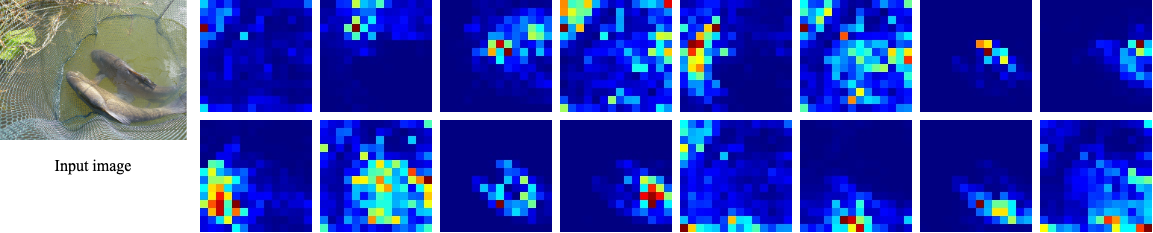
We visualize the attention maps of the first attention layer in the STGM in Figure 3. Because the queries of this layer are spatial initial cluster centers, these attention maps visualize the local semantic information integration by attention. The attention layer groups the semantic information according to the position of initial cluster centers, which ensures to extract fine-grained semantic information and keep the difference among semantic tokens. The attention map in the second attention layer is visualized in Appendix 6.4, which reveals that the network fixedly selects particle semantic tokens to represent global semantic information. We also show the semantic representation of image tokens in the same transformer layer on DeiT in Appendix 6.4. Compared to original image tokens, our semantic tokens in Figure 3 show more high-level semantic information.
Number of transformer layers in STGM.
Two transformer layers are adopted in the STGM by default. The effects of employing different numbers of transformer layers are shown in Table 8. The additional layers are from the ones behind STGM to keep the total number of layers unchanged. More transformer layers do not bring improvement.
The effectiveness of the dumbbell unit.
To verify the effectiveness of our dumbbell unit, we experiment STViT-R without dumbbell units, i.e., STViT equipped with only the recovery module. We employ and transformer layers to construct STGM and the last transformer layers to construct the recovery module in Stage 3. The FLOPs is the same as the full-model STViT-R for fair comparison. The results on the COCO are reported in Table 9. Inferior results demonstrate the effectiveness of the dumbbell unit.
Reusing semantic tokens in dumbbell units.
Semantic tokens are generated in each dumbbell unit. If they are produced only once in the first dumbbell unit and reused as initial cluster centers in the subsequent dumbbell units, the result is shown in Table 9 with a slight performance drop.
5 Conclusion
In this paper, we propose a simple and effective token sparsification method, semantic token vision transformer (STViT). Our method utilizes the clustering property of self-attention to generate a few semantic tokens with high-level information representation to replace the redundant image/video tokens, which can be applied in both global and local vision transformers. By simply configuring the recovery module, our method can be successfully applied to downstream tasks. Extensive experiments demonstrate that our method achieves better accuracy along with less inference time in most cases. The success in downstream tasks significantly boosts the development of token sparsification methods. We hope that this work can inspire more future research to pay much attention to high-level semantic representation in ViTs.
Acknowledgement
This project is supported by the National Research Foundation, Singapore under its NRFF Award NRF-NRFF13-2021-0008, and Mike Zheng Shou’s Start-Up Grant from NUS. The computational work for this article was partially performed on resources of the National Supercomputing Centre, Singapore. Shuning was supported by Alibaba Research Intern Program.
References
- (1) Anurag Arnab, Mostafa Dehghani, Georg Heigold, Chen Sun, Mario Lucic, and Cordelia Schmid. Vivit: A video vision transformer. In Proceedings of the IEEE/CVF international conference on computer vision, pages 6836–6846, 2021.
- (2) Song Bai, Philip Torr, et al. Visual parser: Representing part-whole hierarchies with transformers. arXiv preprint arXiv:2107.05790, 2021.
- (3) Gedas Bertasius, Heng Wang, and Lorenzo Torresani. Is space-time attention all you need for video understanding? In ICML, volume 2, page 4, 2021.
- (4) Zhaowei Cai and Nuno Vasconcelos. Cascade r-cnn: Delving into high quality object detection. In Proceedings of the IEEE conference on computer vision and pattern recognition, pages 6154–6162, 2018.
- (5) Nicolas Carion, Francisco Massa, Gabriel Synnaeve, Nicolas Usunier, Alexander Kirillov, and Sergey Zagoruyko. End-to-end object detection with transformers. In European conference on computer vision, pages 213–229. Springer, 2020.
- (6) Mathilde Caron, Hugo Touvron, Ishan Misra, Hervé Jégou, Julien Mairal, Piotr Bojanowski, and Armand Joulin. Emerging properties in self-supervised vision transformers. In Proceedings of the IEEE/CVF International Conference on Computer Vision, pages 9650–9660, 2021.
- (7) Joao Carreira and Andrew Zisserman. Quo vadis, action recognition? a new model and the kinetics dataset. In proceedings of the IEEE Conference on Computer Vision and Pattern Recognition, pages 6299–6308, 2017.
- (8) Tianlong Chen, Yu Cheng, Zhe Gan, Lu Yuan, Lei Zhang, and Zhangyang Wang. Chasing sparsity in vision transformers: An end-to-end exploration. Advances in Neural Information Processing Systems, 34, 2021.
- (9) Xinlei Chen*, Saining Xie*, and Kaiming He. An empirical study of training self-supervised vision transformers. arXiv preprint arXiv:2104.02057, 2021.
- (10) Yunpeng Chen, Marcus Rohrbach, Zhicheng Yan, Yan Shuicheng, Jiashi Feng, and Yannis Kalantidis. Graph-based global reasoning networks. In Proceedings of the IEEE/CVF Conference on Computer Vision and Pattern Recognition, pages 433–442, 2019.
- (11) Xiangxiang Chu, Zhi Tian, Yuqing Wang, Bo Zhang, Haibing Ren, Xiaolin Wei, Huaxia Xia, and Chunhua Shen. Twins: Revisiting the design of spatial attention in vision transformers. Advances in Neural Information Processing Systems, 34, 2021.
- (12) Zhigang Dai, Bolun Cai, Yugeng Lin, and Junying Chen. Up-detr: Unsupervised pre-training for object detection with transformers. In Proceedings of the IEEE/CVF Conference on Computer Vision and Pattern Recognition, pages 1601–1610, 2021.
- (13) Jia Deng, Wei Dong, Richard Socher, Li-Jia Li, Kai Li, and Li Fei-Fei. Imagenet: A large-scale hierarchical image database. In 2009 IEEE conference on computer vision and pattern recognition, pages 248–255. Ieee, 2009.
- (14) Xiaoyi Dong, Jianmin Bao, Dongdong Chen, Weiming Zhang, Nenghai Yu, Lu Yuan, Dong Chen, and Baining Guo. Cswin transformer: A general vision transformer backbone with cross-shaped windows. arXiv preprint arXiv:2107.00652, 2021.
- (15) Alexey Dosovitskiy, Lucas Beyer, Alexander Kolesnikov, Dirk Weissenborn, Xiaohua Zhai, Thomas Unterthiner, Mostafa Dehghani, Matthias Minderer, Georg Heigold, Sylvain Gelly, Jakob Uszkoreit, and Neil Houlsby. An image is worth 16x16 words: Transformers for image recognition at scale. ICLR, 2021.
- (16) Mohsen Fayyaz, Soroush Abbasi Koohpayegani, Farnoush Rezaei Jafari, Sunando Sengupta, Hamid Reza Vaezi Joze, Eric Sommerlade, Hamed Pirsiavash, and Juergen Gall. Adaptive token sampling for efficient vision transformers. In European Conference on Computer Vision (ECCV), 2022.
- (17) Kaiming He, Georgia Gkioxari, Piotr Dollár, and Ross Girshick. Mask r-cnn. In Proceedings of the IEEE international conference on computer vision, pages 2961–2969, 2017.
- (18) Zilong Huang, Youcheng Ben, Guozhong Luo, Pei Cheng, Gang Yu, and Bin Fu. Shuffle transformer: Rethinking spatial shuffle for vision transformer. arXiv preprint arXiv:2106.03650, 2021.
- (19) Andrew Jaegle, Felix Gimeno, Andy Brock, Oriol Vinyals, Andrew Zisserman, and Joao Carreira. Perceiver: General perception with iterative attention. In International conference on machine learning, pages 4651–4664. PMLR, 2021.
- (20) Zi-Hang Jiang, Qibin Hou, Li Yuan, Daquan Zhou, Yujun Shi, Xiaojie Jin, Anran Wang, and Jiashi Feng. All tokens matter: Token labeling for training better vision transformers. Advances in Neural Information Processing Systems, 34, 2021.
- (21) Zhenglun Kong, Peiyan Dong, Xiaolong Ma, Xin Meng, Wei Niu, Mengshu Sun, Bin Ren, Minghai Qin, Hao Tang, and Yanzhi Wang. Spvit: Enabling faster vision transformers via soft token pruning. arXiv preprint arXiv:2112.13890, 2021.
- (22) Chunyuan Li, Jianwei Yang, Pengchuan Zhang, Mei Gao, Bin Xiao, Xiyang Dai, Lu Yuan, and Jianfeng Gao. Efficient self-supervised vision transformers for representation learning. arXiv preprint arXiv:2106.09785, 2021.
- (23) Xia Li, Zhisheng Zhong, Jianlong Wu, Yibo Yang, Zhouchen Lin, and Hong Liu. Expectation-maximization attention networks for semantic segmentation. In Proceedings of the IEEE/CVF International Conference on Computer Vision, pages 9167–9176, 2019.
- (24) Youwei Liang, Chongjian Ge, Zhan Tong, Yibing Song, Jue Wang, and Pengtao Xie. Not all patches are what you need: Expediting vision transformers via token reorganizations. In International Conference on Learning Representations, 2022.
- (25) Tsung-Yi Lin, Michael Maire, Serge Belongie, James Hays, Pietro Perona, Deva Ramanan, Piotr Dollár, and C Lawrence Zitnick. Microsoft coco: Common objects in context. In European conference on computer vision, pages 740–755. Springer, 2014.
- (26) Ze Liu, Yutong Lin, Yue Cao, Han Hu, Yixuan Wei, Zheng Zhang, Stephen Lin, and Baining Guo. Swin transformer: Hierarchical vision transformer using shifted windows. In Proceedings of the IEEE/CVF International Conference on Computer Vision, pages 10012–10022, 2021.
- (27) Ze Liu, Jia Ning, Yue Cao, Yixuan Wei, Zheng Zhang, Stephen Lin, and Han Hu. Video swin transformer. In Proceedings of the IEEE/CVF Conference on Computer Vision and Pattern Recognition, pages 3202–3211, 2022.
- (28) Xuezhe Ma, Xiang Kong, Sinong Wang, Chunting Zhou, Jonathan May, Hao Ma, and Luke Zettlemoyer. Luna: Linear unified nested attention. Advances in Neural Information Processing Systems, 34:2441–2453, 2021.
- (29) Lingchen Meng, Hengduo Li, Bor-Chun Chen, Shiyi Lan, Zuxuan Wu, Yu-Gang Jiang, and Ser-Nam Lim. Adavit: Adaptive vision transformers for efficient image recognition. arXiv preprint arXiv:2111.15668, 2021.
- (30) Bowen Pan, Rameswar Panda, Yifan Jiang, Zhangyang Wang, Rogerio Feris, and Aude Oliva. Ia-red: Interpretability-aware redundancy reduction for vision transformers. Advances in Neural Information Processing Systems, 34, 2021.
- (31) Yongming Rao, Wenliang Zhao, Benlin Liu, Jiwen Lu, Jie Zhou, and Cho-Jui Hsieh. Dynamicvit: Efficient vision transformers with dynamic token sparsification. Advances in neural information processing systems, 34, 2021.
- (32) Michael S. Ryoo, AJ Piergiovanni, Anurag Arnab, Mostafa Dehghani, and Anelia Angelova. Tokenlearner: Adaptive space-time tokenization for videos. In Advances in Neural Information Processing Systems (NeurIPS), 2021.
- (33) Lin Song, Songyang Zhang, Songtao Liu, Zeming Li, Xuming He, Hongbin Sun, Jian Sun, and Nanning Zheng. Dynamic grained encoder for vision transformers. In Thirty-Fifth Conference on Neural Information Processing Systems, 2021.
- (34) Yehui Tang, Kai Han, Yunhe Wang, Chang Xu, Jianyuan Guo, Chao Xu, and Dacheng Tao. Patch slimming for efficient vision transformers. arXiv preprint arXiv:2106.02852, 2021.
- (35) Hugo Touvron, Matthieu Cord, Matthijs Douze, Francisco Massa, Alexandre Sablayrolles, and Hervé Jégou. Training data-efficient image transformers & distillation through attention. In International Conference on Machine Learning, pages 10347–10357. PMLR, 2021.
- (36) Hugo Touvron, Matthieu Cord, Alexandre Sablayrolles, Gabriel Synnaeve, and Hervé Jégou. Going deeper with image transformers. In Proceedings of the IEEE/CVF International Conference on Computer Vision, pages 32–42, 2021.
- (37) Huiyu Wang, Yukun Zhu, Hartwig Adam, Alan Yuille, and Liang-Chieh Chen. Max-deeplab: End-to-end panoptic segmentation with mask transformers. In Proceedings of the IEEE/CVF Conference on Computer Vision and Pattern Recognition, pages 5463–5474, 2021.
- (38) Pichao Wang, Xue Wang, Hao Luo, Jingkai Zhou, Zhipeng Zhou, Fan Wang, Hao Li, and Rong Jin. Scaled relu matters for training vision transformers. In Proceedings of the AAAI Conference on Artificial Intelligence (AAAI), 2022.
- (39) Wenhai Wang, Enze Xie, Xiang Li, Deng-Ping Fan, Kaitao Song, Ding Liang, Tong Lu, Ping Luo, and Ling Shao. Pyramid vision transformer: A versatile backbone for dense prediction without convolutions. In Proceedings of the IEEE/CVF International Conference on Computer Vision, pages 568–578, 2021.
- (40) Wenxiao Wang, Lu Yao, Long Chen, Binbin Lin, Deng Cai, Xiaofei He, and Wei Liu. Crossformer: A versatile vision transformer hinging on cross-scale attention. arXiv preprint arXiv:2108.00154, 2021.
- (41) Yulin Wang, Rui Huang, Shiji Song, Zeyi Huang, and Gao Huang. Not all images are worth 16x16 words: Dynamic transformers for efficient image recognition. Advances in Neural Information Processing Systems, 34, 2021.
- (42) Yuqing Wang, Zhaoliang Xu, Xinlong Wang, Chunhua Shen, Baoshan Cheng, Hao Shen, and Huaxia Xia. End-to-end video instance segmentation with transformers. In Proceedings of the IEEE/CVF Conference on Computer Vision and Pattern Recognition, pages 8741–8750, 2021.
- (43) Haiping Wu, Bin Xiao, Noel Codella, Mengchen Liu, Xiyang Dai, Lu Yuan, and Lei Zhang. Cvt: Introducing convolutions to vision transformers. In Proceedings of the IEEE/CVF International Conference on Computer Vision, pages 22–31, 2021.
- (44) Weijian Xu, Yifan Xu, Tyler Chang, and Zhuowen Tu. Co-scale conv-attentional image transformers. In Proceedings of the IEEE/CVF International Conference on Computer Vision (ICCV), pages 9981–9990, October 2021.
- (45) Yifan Xu, Zhijie Zhang, Mengdan Zhang, Kekai Sheng, Ke Li, Weiming Dong, Liqing Zhang, Changsheng Xu, and Xing Sun. Evo-vit: Slow-fast token evolution for dynamic vision transformer. In Proceedings of the AAAI Conference on Artificial Intelligence, 2022.
- (46) Jianwei Yang, Chunyuan Li, Pengchuan Zhang, Xiyang Dai, Bin Xiao, Lu Yuan, and Jianfeng Gao. Focal self-attention for local-global interactions in vision transformers, 2021.
- (47) Hongxu Yin, Arash Vahdat, Jose M Alvarez, Arun Mallya, Jan Kautz, and Pavlo Molchanov. A-vit: Adaptive tokens for efficient vision transformer. In Proceedings of the IEEE/CVF Conference on Computer Vision and Pattern Recognition, pages 10809–10818, 2022.
- (48) Tan Yu, Gangming Zhao, Ping Li, and Yizhou Yu. Boat: Bilateral local attention vision transformer. arXiv preprint arXiv:2201.13027, 2022.
- (49) Li Yuan, Yunpeng Chen, Tao Wang, Weihao Yu, Yujun Shi, Zi-Hang Jiang, Francis E.H. Tay, Jiashi Feng, and Shuicheng Yan. Tokens-to-token vit: Training vision transformers from scratch on imagenet. In Proceedings of the IEEE/CVF International Conference on Computer Vision (ICCV), pages 558–567, October 2021.
- (50) David Junhao Zhang, Kunchang Li, Yali Wang, Yunpeng Chen, Shashwat Chandra, Yu Qiao, Luoqi Liu, and Mike Zheng Shou. Morphmlp: An efficient mlp-like backbone for spatial-temporal representation learning. In Computer Vision–ECCV 2022: 17th European Conference, Tel Aviv, Israel, October 23–27, 2022, Proceedings, Part XXXV, pages 230–248. Springer, 2022.
- (51) Songyang Zhang, Xuming He, and Shipeng Yan. Latentgnn: Learning efficient non-local relations for visual recognition. In International Conference on Machine Learning, pages 7374–7383. PMLR, 2019.
- (52) Minghang Zheng, Peng Gao, Renrui Zhang, Kunchang Li, Xiaogang Wang, Hongsheng Li, and Hao Dong. End-to-end object detection with adaptive clustering transformer. arXiv preprint arXiv:2011.09315, 2020.
- (53) Sixiao Zheng, Jiachen Lu, Hengshuang Zhao, Xiatian Zhu, Zekun Luo, Yabiao Wang, Yanwei Fu, Jianfeng Feng, Tao Xiang, Philip HS Torr, et al. Rethinking semantic segmentation from a sequence-to-sequence perspective with transformers. In Proceedings of the IEEE/CVF conference on computer vision and pattern recognition, pages 6881–6890, 2021.
- (54) Jingkai Zhou, Pichao Wang, Fan Wang, Qiong Liu, Hao Li, and Rong Jin. Elsa: Enhanced local self-attention for vision transformer. arXiv preprint arXiv:2112.12786, 2021.
- (55) Xizhou Zhu, Weijie Su, Lewei Lu, Bin Li, Xiaogang Wang, and Jifeng Dai. Deformable detr: Deformable transformers for end-to-end object detection. In International Conference on Learning Representations, 2020.
- (56) Zhuofan Zong, Kunchang Li, Guanglu Song, Yali Wang, Yu Qiao, Biao Leng, and Yu Liu. Self-slimmed vision transformer. In Computer Vision–ECCV 2022: 17th European Conference, Tel Aviv, Israel, October 23–27, 2022, Proceedings, Part XI, pages 432–448. Springer, 2022.
6 Appendix
6.1 Computational complexity analysis
Global vision transformer (DeiT).
We define that the number of image tokens is N, the number of semantic tokens is M, and their dimension is C. The patch embedding layer is neglected. The computational complexity of a global transformer processing image tokens (IT) is:
| (7) |
The computational complexity of a global transformer processing semantic tokens (ST) is:
| (8) |
The relationships between computational complexity and token number in attention and FFN are quadratic and linear, respectively. Due to the , our method significantly reduces the cost of transformers, especially the attention. The computational complexity of STGM is:
| (9) |
In global vision transformers, our STGM is also an efficient module. The computational complexity of whole DeiT and our STViT-DeiT are:
| (10) |
| Model | Metrics | Base | No. of semantic tokens | ||
|---|---|---|---|---|---|
| 36 | 49 | 100 | |||
| STViT-LV-ViT-S | Top-1 Acc(%) | 83.3 | 82.7(-0.6) | 82.8(-0.5) | 83.1(-0.2%) |
| FLOPs(G) | 6.6 | 3.69(-44%) | 3.91(-41%) | 4.62(-30%) | |
| Throughput(img/s) | 1159 | 2073(+78%) | 1933(+72%) | 1592(+37%) | |
Local vision transformer (Swin).
We define that the number of image tokens (IT) is N, the number of image tokens in each window is W, the number of semantic tokens (ST) in each window is M, and their dimension is C. We only compute the computational complexity in each transformer. The computational complexity of a local transformer processing image tokens (IT) is:
| (11) |
The computational complexity of a local transformer processing image tokens (ST) is:
| (12) |
Swin makes the computational complexity linear to token number, while our method further reduces the computational complexity. The computational complexity of STGM is:
| (13) |
6.2 The results on LV-ViT
Setting.
In LV-ViT jiang2021all, by default, the STGM employs the and transformer layers of LV-ViT-S (with 16 layers in total). We downsample the token labels to match the size of our semantic tokens.
Results.
The main results are shown in Table 10. Token labelling in LV-ViT is not friendly for our method. Token labelling emphasizes the importance of all the output tokens and advocates that each output token should be associated with an individual location-specific label jiang2021all, while our semantic tokens generated by clustering emphasize high-level semantic information. However, we still achieve good performance. In Table 11, we compare our STViT with the state-of-the-art token sparsification method EViT liang2022evit on LV-ViT-S. Results indicate that our method outperforms it.
6.3 Applications in semantic segmentation
Settings.
ADE20K is a widely-used semantic segmentation dataset, including a broad range of 150 semantic classes. It has 25K images in total, with 20K for training, 2K for validation, and 3K for testing. UperNet in mmseg is utilized as our base framework. The is set to . Models are trained for 240K iterations. All the other settings follow the Swin Transformer liu2021swin.
Comparison to Swin Transformers.
Table 12 presents the results of STViT-R-Swin on semantic segmentation. With similar FLOPs reduction, the drop on mIoU is larger compared with those in object detection tasks, which shows that our method still has a gap on dense prediction compared to the full-token network.
We analyze the relatively poor performance from two views. First, the STGM strictly prunes more than 80% tokens by attention, which remains the high-level semantic information but loses nearly all the detailed information. Semantic segmentation is a dense pixel-level classification task, and the semantic tokens are difficult to enhance the pixel-level representation. Second, our spatial pooling layer with large kernel size in STGM and self-attention layers can be regarded as low-frequency filters. STGM filters most high-frequency information, which is necessary for semantic segmentation.
6.4 Additional visualization
We visualize the attention map of the second attention layer in STGM in Figure 4(a). The shape of attention map is , where , and . The results of the attention computation between semantic tokens (queries) and semantic tokens (keys) are shown in the most left 16 columns, and the rest columns show the computation between semantic tokens and image tokens . The figure shows that the second semantic token highlights the region of semantic tokens, while other semantic tokens highlight the image tokens. Figure 4(c) visualizes the attention maps in the self-attention layers after STGM. The second semantic token is incorporated by the majority of semantic tokens. These phenomenons illustrate that the second semantic token focuses on more global semantic information, which further verifies our global cluster center initialization can guide the semantic tokens to extract global semantic information. The phenomenons in Figure 4(a) and Figure 4(c) nearly emerge in all the images.
Neglecting the most left 16 columns of Figure 4(a), we reshape it into 16 attention maps like Figure 3 and show them in Figure 4(b). Thanks to the clustering of second attention and global initialization G, we can see that the semantic information is more accurate and meaningful.
We visualize the attention maps of semantic tokens with single global initialization in Figure 4(d). Without spatial initialization, the response regions are more global and similar. In contrast, our semantics of each semantic token are associated with the specific spatial location, which is the basis to allow our method to be applied in local self-attention and downstream tasks. Additionally, our attention maps contain more recognized and diverse semantic information, reflecting the effectiveness of our spatial initialization.
| Method | Top-1 Acc | FLOPs(G) |
|---|---|---|
| EViT liang2022evit | 82.5(-0.8) | 3.9(-41%) |
| EViT liang2022evit | 83.0(-0.3) | 4.7(-29%) |
| STViT(Ours) | 82.7(-0.6) | 3.7(-44%) |
| STViT(Ours) | 83.1(-0.2) | 4.6(-30%) |
6.5 Additional ablation study
All the following experiments of STViT and STViT-R are conducted on DeiT-S and Swin-S unless otherwise specified, respectively.


The position of STGM.
The effects of different position of STGM are shown in Table 13. Two transformer layers are employed in STGM in all the experiments. We can see that the performance achieves improvement with appropriately moving the STGM towards deep layers due to better features of image tokens.
Positional encoding.
We try to apply positional encoding to our semantic tokens. Table 14 shows comparisons of different positional encoding methods, including learned positional encoding, conditional positional encoding, and relative positional encoding liu2021swin. All the positional encoding methods do not work on DeiT-S and Swin-T, even though relative positional encoding improves Swin-T by 1.2%. These experiments demonstrate that the interaction between our semantic tokens depends on high-level semantic information and nearly does not use position relationships.
| Method | Backbone | mIoU | FLOPs(G) |
|---|---|---|---|
| UperNet | Swin-S | 49.3 | 49 |
| UperNet | STViT-R-Swin-S | 48.3 | 34(-31%) |
| UperNet | Swin-B | 49.7 | 87 |
| UperNet | STViT-R-Swin-B | 48.9 | 60(-31%) |
| Pos. | 3-5 | 4-6 | 5-7 | 7-9 | 8-10 | 10-12 |
|---|---|---|---|---|---|---|
| Top-1 Acc(%) | 79.3 | 79.8 | 79.8 | 80.3 | 80.3 | 79.8 |
| FLOPs(G) | 1.56 | 1.91 | 2.25 | 2.95 | 3.30 | 4.00 |
| STViT-DeiT-S Acc | STViT-Swin-T Acc | |
|---|---|---|
| Learned | 79.6 | 81.5 |
| Conditional | 79.7 | 81.4 |
| Relative | 79.8 | 81.3 |
| No pos. | 79.8 | 81.5 |
Alternative schemes of spatial pooling.
We use an intra and inter-window spatial pooling in STGM to generate initial cluster centers, which adaptively save meaningful semantic information and avoids overlap between adjacent windows as much as possible. Furthermore, we explore more spatial pooling schemes, including: (i) spatial pooling with large-size kernel and overlap, (ii) multi-scale spatial pooling, and (iii) adaptive spatial pooling. We adopt 25 semantic tokens in these experiments. In (i), the kernel size and overlap are set to 6 and 4, respectively. In (ii), we use two adaptive pooling layers which produce 9 and 16 tokens separately. The results are presented in Table 15 on DeiT-T. We can see that overlap and multiple scales cannot boost the performance, which also demonstrates that discrete semantic tokens with high-level semantic information benefit our method.
| Scheme i | Scheme ii | Adaptive spatial pooling | Ours | |
| Top-1 Acc(%) | 71.6 | 71.7 | 71.9 | 72.2 |
6.6 Cluster center recovery by self attention
We present an analysis showing how cluster centers are recovered through the attention mechanism. Let be the number of clusters. Let be the Gaussian distributions, with center and covariance matrix . Let be the data points independently sampled from . Given data points , of course without knowing the association of each data point to its underlying Gaussian distribution, our goal is to recover the underlying cluster centers . We assume that all the center vectors of Gaussian distributions are well separated, i.e. if . For the convenience of study, we assume .
Let the initialized cluster centers, with all the cluster centers being well normalized. Define as the gap for any initialized to the target cluster centers than to other clusters , i.e.
The new cluster centers are estimated through the self-attention mechanism, i.e.
where is a scaling factor and is defined as
Theorem 1
With sufficiently large and , with a probability , we have
Define . We have
We first bound . Since and , we know that . Hence, with a probability , we have
Since
we have, with a probability ,
With large enough , we have
and therefore
where
Here is a universal constant.
We second bound . We write each , where and is a dimensional Gaussian vector. We have
Since , we have . Using the concentration of distribution, we have, with a probability
To bound , following the same procedure, we have, with a probability
Since
and
We thus have, with a probability ,
When is sufficiently large, we have, with a probability
where . By putting them together, with a probability , we have
with and
Finally, we have, with a probability
Using the same analysis, we have, with a probability ,
Now, we can bound . We have
To further develop the bound for , we have
and
We thus have
By choosing , and by assuming is significantly larger than , we have
implying that