Latent space approaches to aggregate network data

Latent space models endow each node $i$ in a population of $n$ nodes with coordinates $z_{i}\in\mathbb{R}^{q}$ in a $q$-dimensional latent space [2]. The nodes’ positions in the latent space encode how they relate to one another. We use an adjacency matrix $y$ to represent connections between nodes such that $y_{ij}=1$ if node $j$ is connected to node $i$ and $y_{ij}=0$ otherwise. The probability for nodes $i$ and $j$ to connect is

$$p\left(y_{ij}=1\mid z_{i},z_{j},\theta\right)=\lambda\left(z_{i},z_{j},\theta\right),$$

where $\theta$ parameterises the connectivity kernel $\lambda$, which typically decays with increasing separation between the nodes. Connections are conditionally independent given the latent coordinates $z$. The kernel is assumed to be symmetric with respect to exchange of coordinates, i.e. $\lambda\left(z_{i},z_{j},\theta\right)=\lambda\left(z_{j},z_{i},\theta\right)$. We consider unweighted, directed networks, but subsequent results generalise to weighted and undirected networks (see appendix A for details).

Each node $i$ belongs to one of $r$ groups $g_{i}$, and members of the same group have a common coordinate distribution in the latent space, i.e.

$$z_{i}\mid\mu,\sigma,g_{i}\sim\mathsf{Normal}\left(\mu_{g_{i}},\sigma^{2}_{g_{i}}\right),$$

where $\mu_{g}\in\mathbb{R}^{q}$ is the centre of group $g$ and $\sigma^{2}_{g}>0$ is its variance. This setup closely follows the model-based clustering approach for latent space models developed by [14].

In contrast to latent space cluster models [14] and community detection algorithms [15], which are designed to assign nodes to latent groups given the individual-level network $y$, we assume that groups are defined a priori and that individual connections remain hidden. For example, groups could be defined by members having certain properties in common, such as sex, age, physical location, or a combination thereof. Only aggregate connections $Y$ between groups are observable. In particular, the number of connections from group $b$ to group $a$ is

$$Y_{ab}=\sum_{i\neq j}\delta_{ag_{i}}\delta_{bg_{j}}y_{ij},$$

(1)

where $\delta_{ab}$ is the Kronecker delta.

To complete the model, we impose a prior on the centres of groups

$$\mu\sim\mathsf{Normal}\left(0,\tau^{2}\right),$$

where $\tau^{2}>0$ is the population variance. The population prior ensures that disconnected groups retain finite coordinates when the model is fit to data. We use a half-Cauchy prior for the population and group scales $\tau$ and $\sigma$, respectively [16]. The prior for kernel parameters $\theta$ will be discussed in section 2.4. An example of a synthetic network generated by the model is shown in panel (a) of fig. 1.

Because the individual connections $y$ and latent coordinates $z$ are not observable, we are interested in the marginal likelihood

$$p\left(Y\mid\mu,\sigma,g,\theta\right)=\int dz\,p\left(Y\mid z,\theta\right)p\left(z\mid\mu,\sigma,g\right).$$

The distribution of $Y_{ab}$ given kernel parameters $\theta$ and node coordinates $z$ is a Poisson-binomial distribution, a generalisation of the binomial distribution allowing different probabilities for each trial. Its likelihood is difficult to evaluate, and the integral is intractable. However, we can evaluate the marginal moments of the aggregate connection volumes $Y$ which we will use to approximate the marginal likelihood.

Taking the expectation of eq. 1 with respect to node coordinates $z$ and connections $y$ (denoted by $\left\langle\cdot\right\rangle_{y,z}$), we find

$$\left\langle Y_{ab}\right\rangle_{y,z}=\begin{cases}n_{a}\left(n_{a}-1\right)\left\langle\lambda_{ij}\right\rangle_{z}&\text{if }a=b\\ n_{a}n_{b}\left\langle\lambda_{ij}\right\rangle_{z}&\text{otherwise},\end{cases}$$

(2)

where $n_{g}$ is the number of nodes in group $g$, we have used $\lambda_{ij}=\lambda\left(z_{i},z_{j},\theta\right)$ for notational convenience, $z_{i}\sim\mathsf{Normal}\left(\mu_{a},\sigma_{a}^{2}\right)$, and $z_{j}\sim\mathsf{Normal}\left(\mu_{b},\sigma_{b}^{2}\right)$.

The second moment of within-group connections is

$$\left\langle Y_{aa}^{2}\right\rangle_{y,z}=\sum_{i\neq j,k\neq l}\left\langle y_{ij}y_{kl}\right\rangle_{y,z},$$

(3)

where all nodes $i$, $j$, $k$, and $l$ belong to the same group $a$. Since the adjacency matrix elements $y_{ij}$ are independent Bernoulli random variables,

$$\left\langle y_{ij}y_{kl}\right\rangle_{y,z}=\begin{cases}\left\langle\lambda_{ij}\right\rangle_{z}&\text{if }i=k\text{ and }j=l\\ \left\langle\lambda_{ij}\lambda_{kl}\right\rangle_{z}&\text{otherwise}.\end{cases}$$

(4)

Substituting into eq. 3 yields

	$\displaystyle\left\langle Y_{aa}^{2}\right\rangle_{y,z}=n_{a}\left(n_{a}-1\right)$	$\displaystyle\left[\left\langle\lambda_{ij}\right\rangle_{z}+\left\langle\lambda_{ij}^{2}\right\rangle_{z}+4(n_{a}-2)\left\langle\lambda_{ij}\lambda_{il}\right\rangle_{z}\right.$		(5)
		$\displaystyle\left.+(n_{a}-2)(n_{a}-3)\left\langle\lambda_{ij}\right\rangle_{z}^{2}\right],$

where repeated indices refer to the same node, distinct indices refer to different nodes, and we have used the symmetry of the kernel to simplify $\lambda_{ij}\lambda_{ji}=\lambda_{ij}^{2}$. The prefactors account for the number of times different terms occur (see appendix A for details). The variance of within-group connections is thus

	$\displaystyle\var_{y,z}Y_{aa}$	$\displaystyle=\left\langle Y_{aa}\right\rangle_{y,z}-\left\langle Y_{aa}\right\rangle_{y,z}^{2}$
		$\displaystyle=n_{a}\left(n_{a}-1\right)\left[\left\langle\lambda_{ij}\right\rangle_{z}\left(1-\left\langle\lambda_{ij}\right\rangle_{z}\right)+\var_{z}\lambda_{ij}+4(n_{a}-2)\cov_{z}\left(\lambda_{ij},\lambda_{il}\right)\right].$		(6)

The first term accounts for variance due to individual connections, the second term captures reciprocity, and the last term encodes variance due to two edges sharing a common node. Similarly, the variance of between-group connections is

	$\displaystyle\var_{y,z}Y_{ab}=n_{a}n_{b}$	$\displaystyle\left[\left\langle\lambda_{ij}\right\rangle_{z}\left(1-\left\langle\lambda_{ij}\right\rangle_{z}\right)+(n_{b}-1)\cov_{z}\left(\lambda_{ij},\lambda_{il}\right)\right.$		(7)
		$\displaystyle\left.+(n_{a}-1)\cov_{z}\left(\lambda_{ij},\lambda_{kj}\right)\right],$

where nodes $i$ and $k$ belong to group $a$ and nodes $j$ and $l$ belong to group $b$. Similar to eq. 6, the first term captures individual connection variance. The second and third terms account for variance due to two edges sharing a common node in group $a$ and $b$, respectively. In contrast to eq. 6, there is no reciprocity term because we consider directed connections from one group to another.

Having derived the marginal mean and variance for within- and between-group connections, we approximate the likelihood by independent beta-binomial distributions. Like Poisson-binomial distributions, beta-binomial distributions generalise the binomial distribution and can model overdispersion, but their likelihood is tractable. In particular,

	$\displaystyle p\left(Y_{ab}\mid\mu,\sigma,\theta\right)$	$\displaystyle\approx\mathsf{BetaBinomial}\left(Y_{ab}\mid t_{ab},\alpha_{ab},\beta_{ab}\right),$		(8)
	$\displaystyle\text{where }t_{ab}$	$\displaystyle=\begin{cases}n_{a}(n_{a}-1)&\text{if }a=b\\ n_{a}n_{b}&\text{otherwise}\end{cases}$

is the number of trials and ensures that the beta-binomial distributions have the same domain as $Y$. For notational convenience, we have omitted the explicit dependence of the shape parameters $\alpha$ and $\beta$ on $\mu$, $\sigma$, and $\theta$. We choose the parameters by matching moments with the mean in eq. 2 and variances in eqs. 6 and 7 (see appendix B for details).

Finally, we arrive at the approximate marginal likelihood

$$p\left(Y\mid\mu,\sigma,\theta\right)\approx\prod_{a,b=1}^{r}\mathsf{BetaBinomial}\left(Y_{ab}\mid t_{ab},\alpha_{ab},\beta_{ab}\right).$$

(9)

The approximation neglects correlations between different connection volumes, but eq. 9 yields a sufficient approximation of the likelihood for inference in practice. These correlations are not unique to fully aggregated network data; they are also present in the partially aggregated data considered by [12], who have similarly not modelled them.

We need to obtain expressions for the moments of the connectivity kernel on the right-hand side of eq. 4 to evaluate the approximate likelihood. Latent space models commonly use logistic kernels [2, 14], but their moments are intractable for the Gaussian coordinate distributions of the latent space cluster model. Following [3], we use a Gaussian kernel of the form

$$\lambda\left(x,y,\theta\right)=\theta\exp\left(-\frac{\left|x-y\right|^{2}}{2}\right),$$

where the propensity parameter $0\leq\theta\leq 1$ controls the overall edge density. We do not include a spatial scale parameter in the kernel because the likelihood is invariant under a global rescaling. For two nodes $i$ and $j$ respectively belonging to groups $a$ and $b$, the expected probability to connect is

$$\left\langle\lambda_{ij}\right\rangle_{z}=\frac{\theta}{\left(1+\sigma_{a}^{2}+\sigma_{b}^{2}\right)^{q/2}}\exp\left(-\frac{\left|\mu_{a}-\mu_{b}\right|^{2}}{2\left(1+\sigma_{a}^{2}+\sigma_{b}^{2}\right)}\right).$$

A detailed derivation of the results presented in this section can be found in appendix C.

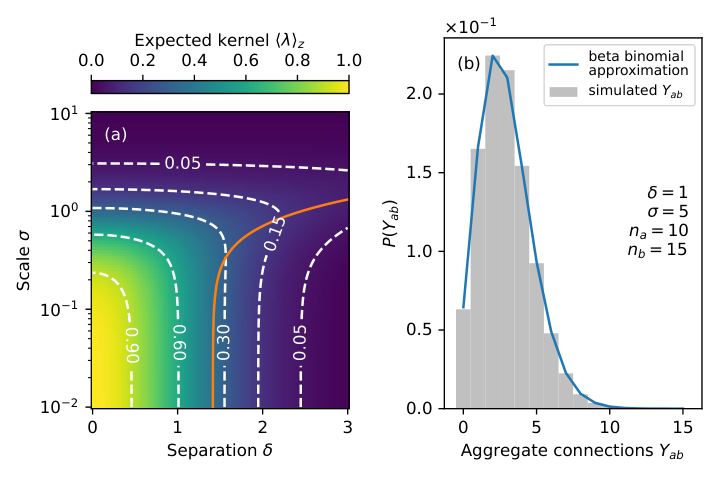
The expected kernel decreases exponentially with increasing separation $\delta=\left|\mu_{a}-\mu_{b}\right|$ between the two clusters, as shown in fig. 2 (a). However, for a given separation, there is an optimal scale that maximises the expected kernel. Assuming the two clusters have a common scale $\sigma_{a}=\sigma_{b}=\sigma$, the kernel is maximised by

$$\sigma^{2}_{\max}=\frac{\max\left(\delta^{2}-q,0\right)}{2q}.$$

On the one hand, when $\sigma<\sigma_{\max}$, the two clusters are isolated islands in the latent space, and the expected connection probability is small. On the other hand, when $\sigma>\sigma_{\max}$, the clusters overlap but are diffuse. The population density in the latent space is thus low, diminishing the likelihood of connections. At the optimal scale, the the two clusters overlap and the density remains sufficiently high for connections to form. When the squared distance is smaller than the dimensionality of the latent space, the connectivity is maximised by two point-mass distributions: for nonzero scales, any additional connectivity due to overlap between the distributions is thwarted by the increased separation between the peripheries.

The additional statistics required to evaluate the moments of aggregate connection volumes in eqs. 6 and 7 are

	$\displaystyle\left\langle\lambda_{ij}^{2}\right\rangle_{z}$	$\displaystyle=\frac{\theta^{2}}{\left(1+2\sigma_{a}^{2}+2\sigma_{b}^{2}\right)^{q/2}}\exp\left(-\frac{\left|\mu_{a}-\mu_{b}\right|^{2}}{1+2\sigma_{a}^{2}+2\sigma_{b}^{2}}\right)$
	$\displaystyle\left\langle\lambda_{ij}\lambda_{il}\right\rangle_{z}$	$\displaystyle=\frac{\theta^{2}}{\left[(1+2\sigma_{a}^{2}+\sigma_{b}^{2})(1+\sigma_{b}^{2})\right]^{q/2}}\exp\left(-\frac{\left|\mu_{a}-\mu_{b}\right|^{2}}{1+2\sigma_{a}^{2}+\sigma_{b}^{2}}\right),$		(10)

where node $i$ belongs to group $a$ and nodes $j\neq l$ belong to group $b$ (see appendix C for detailed derivations).

Having obtained expressions for the kernel moments in eq. 4, we can evaluate the aggregate mean in eq. 2 and variances in eqs. 7 and 6. To evaluate the quality of the moment-matched beta-binomial approximation in eq. 8, we compared the approximation with the empirical distribution of $10^{5}$ independent realisations of $Y_{ab}$ obtained by simulating the data generation process at the level of individual nodes and connections. We considered two clusters with 10 and 15 nodes, respectively, shared scale $\sigma=5$, and separation $\delta=1$. The beta-binomial likelihood approximated the empirical distribution well, as shown in panel (b) of fig. 2.

We sought to infer the parameters (comprising cluster coordinates $\mu$, scales $\sigma$, population scale $\tau$, and propensity $\theta$) from data given only aggregate network data $Y$. To this end, we used the probabilistic programming framework Stan [17] to draw samples from the posterior distribution

$$p\left(\mu,\tau,\sigma,\theta\mid Y\right)\propto p\left(Y\mid\mu,\sigma,\theta\right)p\left(\mu\mid\tau\right)p\left(\tau\right)p\left(\sigma\right)p\left(\theta\right).$$

We used eq. 9 to approximate the first term and assumed a uniform prior on the unit interval for the propensity $\theta$. The priors for $\mu$, $\tau$, and $\sigma$ are specified in section 2.1.

The model is only identifiable up to rotations and translations in the latent space because the likelihood solely depends on distances in the space rather than absolute coordinates. Because Stan attempts to explore the entire posterior distribution, the sampler spent considerable resources exploring all possible rotations of the latent space. To reduce rotational summary, we re-parameterised the cluster centres $\mu$ such that, without loss of generality, the first $q$ centres were axis-aligned. Translational symmetry was attenuated by the population-level prior $p\left(\mu\mid\tau\right)$ centred at the origin. Furthermore, the propensity parameter $\theta$ was heavily correlated with the group scales $\sigma$ and population scale $\tau$ in the posterior because small propensities can be compensated for by smaller scales, increasing the density of nodes in the latent space. The presence of groups with different scales attenuated the degeneracy, but the parameters remained weakly identified. See appendix D for a more detailed discussion of the parameterisation.

Having drawn samples from the posterior, we aligned them using a rigid Procrustes transformation [2], i.e. samples were translated and rotated to minimise the mean squared error between samples of group locations $\mu$. Aligning the samples was necessary for common posterior summary statistics (such as posterior means or medians) to be applicable.

References

- [1] Mark Newman “Networks” Oxford University Press, 2018 DOI: 10.1093/oso/9780198805090.001.0001
- [2] Peter Hoff, Adrian Raftery and Mark Handcock “Latent Space Approaches to Social Network Analysis” In J. Am. Stat. Assoc. 97.460, 2002, pp. 1090–1098 DOI: 10.1198/016214502388618906
- [3] Riccardo Rastelli, Nial Friel and Adrian. Raftery “Properties of latent variable network models” In Netw. Sci. 4.4, 2016, pp. 407–432 DOI: 10.1017/nws.2016.23
- [4] Adrian. Raftery, Xiaoyue Niu, Peter. Hoff and Ka Yeung “Fast Inference for the Latent Space Network Model Using a Case-Control Approximate Likelihood” In J. Comput. Graph. Stat. 21.4, 2012, pp. 901–919 DOI: 10.1080/10618600.2012.679240
- [5] Michael Salter-Townshend and Thomas Murphy “Variational Bayesian inference for the Latent Position Cluster Model for network data” In Comput. Stat. Data Anal. 57.1, 2013, pp. 661–671 DOI: 10.1016/j.csda.2012.08.004
- [6] David Lazer et al. “Meaningful measures of human society in the twenty-first century” In Nature 595.7866, 2021, pp. 189–196 DOI: 10.1038/s41586-021-03660-7
- [7] Scott. Golder and Michael. Macy “Digital Footprints: Opportunities and Challenges for Online Social Research” In Annu. Rev. Sociol. 40.1, 2014, pp. 129–152 DOI: 10.1146/annurev-soc-071913-043145
- [8] Lars Backstrom, Cynthia Dwork and Jon Kleinberg “Wherefore Art Thou R3579x? Anonymized Social Networks, Hidden Patterns, and Structural Steganography” In World Wide Web 16, 2007, pp. 181–190 DOI: 10.1145/1242572.1242598
- [9] Michal Kosinski, David Stillwell and Thore Graepel “Private traits and attributes are predictable from digital records of human behavior” In Proc. Natl. Acad. Sci. U.S.A. 110.15, 2013, pp. 5802–5805 DOI: 10.1073/pnas.1218772110
- [10] Danah Boyd and Kate Crawford “Critical questions for big data” In Inf. Commun. Soc. 15.5, 2012, pp. 662–679 DOI: 10.1080/1369118X.2012.678878
- [11] Lawrence. Cox “Suppression Methodology and Statistical Disclosure Control” In J. Am. Stat. Assoc. 75.370, 1980, pp. 377–385 DOI: 10.1080/01621459.1980.10477481
- [12] Tyler. McCormick and Tian Zheng “Latent Surface Models for Networks Using Aggregated Relational Data” In J. Am. Stat. Assoc. 110.512, 2015, pp. 1684–1695 DOI: 10.1080/01621459.2014.991395
- [13] Emily Breza, Arun. Chandrasekhar, Tyler. McCormick and Mengjie Pan “Using Aggregated Relational Data to Feasibly Identify Network Structure without Network Data” In Am. Econ. Rev. 110.8, 2020, pp. 2454–2484 DOI: 10.1257/aer.20170861
- [14] Mark. Handcock, Adrian. Raftery and Jeremy. Tantrum “Model-based clustering for social networks” In J. R. Stat. Soc. A 170.2, 2007, pp. 301–354 DOI: 10.1111/j.1467-985X.2007.00471.x
- [15] Santo Fortunato “Community detection in graphs” In Phys. Rep. 486.3, 2010, pp. 75–174 DOI: 10.1016/j.physrep.2009.11.002
- [16] Nicholas. Polson and James. Scott “On the Half-Cauchy Prior for a Global Scale Parameter” In Bayesian Anal. 7.4, 2012, pp. 887–902 DOI: 10.1214/12-BA730
- [17] Bob Carpenter et al. “Stan: A Probabilistic Programming Language” In J. Stat. Softw. 76.1, 2017, pp. 1–32 DOI: 10.18637/jss.v076.i01
- [18] James Moody “The structure of adolescent social relations: modeling friendship in dynamic social settings”, 1999
- [19] Alp Kucukelbir et al. “Automatic Differentiation Variational Inference” In J. Mach. Learn. Res. 18.1, 2017, pp. 430–474 DOI: 10.5555/3122009.3122023
- [20] Cristopher. Bishop “Pattern recognition and machine learning” Springer, 2006
- [21] Brian Ball and Mark Newman “Friendship networks and social status” In Netw. Sci. 1.1, 2013, pp. 16–30 DOI: 10.1017/nws.2012.4
- [22] Peter. Hoff “Multiplicative latent factor models for description and prediction of social networks” In Comput. Math. Organ. Theory 15.4, 2008, pp. 261 DOI: 10.1007/s10588-008-9040-4
- [23] Peter Hoff “Additive and Multiplicative Effects Network Models” In Stat. Sci. 36.1, 2021, pp. 34–50 DOI: 10.1214/19-STS757
- [24] T Hoffmann and N Jones “Kernel-based approaches to large social networks” In NetMob, 2017, pp. 102–104
Appendix A Statistics of aggregate relational data