Learning for Precision Motion of an Interventional X-ray System: Add-on Physics-Guided Neural Network Feedforward Control^footnoteinfoThis work is supported by Topconsortia voor Kennis en Innovatie (TKI), and ASML and Philips Engineering Solutions.

The considered interventional X-ray system is depicted in Fig. 1. While it has 3 degrees of freedom, this paper considers only the roll axis. The roll axis body rotates in a roller-based guidance attached to the sleeve, thus positioning the X-ray source and detector in this dimension. It is driven by a permanent magnet DC motor and an amplifier with a maximum input of 5 [V] through a transmission consisting of gears and belts. The rotation is measured using an incremental encoder with an effective resolution of $0.0119$ [deg]. Encoder measurements and power for the X-ray source are supplied through a cable at the side of the setup, which is acting as a dynamic link. The software runs on a Speedgoat system with $T_{s}=\frac{1}{500}$ [s].

This mechanical design, motivated and constrained by the use around medical personnel, introduces the following hard-to-model nonlinear dynamics.

1. 1.

   The mass distribution is unbalanced, resulting in configuration-dependent gravitational forces.

2. 2.

   The cable acts as a configuration-dependent inertia, and is tensioned for large negative $\theta$, acting as a one-sided spring.

3. 3.

   The friction characteristics in the guidance depend on the normal forces acting on the contact surface of the rollers, and are thus configuration-dependent.

The configuration-dependent gravitational forces can be quantitatively captured by a physical model. However, the exact way these parasitic cable and friction forces depend on the configuration $\theta$ is exceptionally hard to model from a physics-based perspective, limiting the tracking performance of physical-model-based feedforward control.

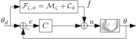
The main dynamics of the interventional X-ray system, i.e., the configuration-dependent gravitational forces, can be described by physics, but the cable and friction forces are only qualitatively understood and hard to model. Therefore, the physical model $\mathcal{M}_{\zeta}$ with parameters $\zeta$ is complemented by a neural network $\mathcal{C}_{\phi}$ to learn these hard-to-model dynamics, resulting in a parallel PGNN feedforward controller $\mathcal{F}_{\zeta,\phi}$, see Fig. 2. Additionally, a simple PD feedback controller is employed to compensate both unknown external disturbances as well as dynamics uncompensated by the PGNN feedforward controller.

The aim of this paper is to learn the parameters $\zeta,\phi$ of the PGNN feedforward controller (defined in the next section) that compensate the hard-to-model cable and friction force, thereby increasing tracking performance, in such a way that $\mathcal{M}_{\zeta}$ stays interpretable and $\mathcal{C}_{\phi}$ increases performance by learning only unmodeled dynamics, i.e., while ensuring complementarity. In this paper, an inverse system identification approach is taken, in which $\zeta,\phi$ are learned based on a dataset $\mathcal{D}$ describing the system’s dynamics consisting of inputs $\hat{u}(k)$ corresponding to outputs $\theta(k)$ with $k=1,\ldots,N$ that has been obtained in advance, e.g., feedback or iterative learning control data.

To compensate hard-to-model dynamics, the feedforward controller $\mathcal{F}_{\zeta,\phi}$ is parametrized as the parallel combination of a physical model $\mathcal{M}_{\zeta}$ and complementary neural network $\mathcal{C}_{\phi}$ according to

and is visualized in Fig. 3. The physical model $\mathcal{M}_{\zeta}$ with parameters $\zeta$ represents prior knowledge of the physical process through encapsulating quantitatively known dynamics. The physical model is complemented by a universal function approximator $\mathcal{C}_{\phi}$ with parameters $\phi$, here chosen as a neural network, such that it can learn dynamics not included in the physical model.

The physical model $\mathcal{M}_{\zeta}$ constitutes an equation of motion describing the relation between the generalized coordinate $\theta$ and the input $u$ derived from first-principles modeling (de Vos 2022). More specifically, assuming that inputs are confined within actuator limits and ignoring drivetrain flexibilities, the equation of motion for $\theta$ is given by

Here, $d\in\mathbb{R}_{\geq 0}$ is the viscous damping coefficient,

the inertia of the roll axis, and

the gravity contribution. Coordinates $y,z\in\mathbb{R}$ represent the offset of the center of mass with respect to the point of rotation, and $\phi$ the known orientation of the roll axis out of the vertical plane.

The required feedforward signal can be obtained by evaluating the right-hand-side for a given reference $\theta_{d}$ and discrete-time derivatives $\dot{\theta}_{d}$. Thus, the physical-model-based feedforward controller $\mathcal{M}_{\zeta}:\theta_{d}\rightarrow f_{\mathcal{M}}$ is given by

with physical parameters

The neural network $\mathcal{C}_{\phi}$ consists of a feedforward neural network (FNN) acting on a physics-guided input vector. By the universal approximation theorem (Goodfellow et al. 2016), $\mathcal{C}_{\phi}$ can represent any continuous function on a bounded interval up to arbitrary precision, such that it can learn hard-to-model dynamics, such as cable forces, from data.

More specifically, the neural network feedforward controller $\mathcal{C}_{\phi}:\theta_{d}\rightarrow f_{\mathcal{C}}$ is defined as

The FNN $g_{\phi}:T(\theta_{d}(k))=x\rightarrow f_{\mathcal{C}}(k)$ is given by a fully connected multilayer perceptron (MLP) of $L$ hidden layers and a linear output layer without bias, i.e.,

in which $W^{l},b^{l}$ are appropriately sized weight matrices and bias vectors defining affine mappings, and $\sigma$ is an element-wise activation function acting on this affine mapping, such as a sigmoid, hyperbolic tangent ($\tanh$) or rectified linear unit (ReLU). The full MLP $g_{\phi}$ then is the repeated application of affine and nonlinear transformations.

The physics-guided input transformation $T$ encodes prior qualitative knowledge on the hard-to-model dynamics and is defined as

with

and $\mathrm{relay}(x(0))=0$. It transforms $\theta_{d}$ such that the input to $g_{\phi}$ contains all relevant physical quantities to make predictions about the required force. For example, $T(\theta_{d}(k))$ contains the reference velocity $\dot{\theta}_{d}$ to learn complex friction characteristics, and a relay of the velocity to approximate hysteresis characteristics without requiring a recurrent network architecture, thereby greatly simplifying optimization.

To illustrate unidentifiability, the least-squares cost function is decomposed in two orthogonal subspaces, one spanned by the physical model (locally, given some fixed parameter) and one as its orthogonal complement, from which it is apparent that the neural network can have a contribution in the subspace spanned by the physical model, resulting in unidentifiability.

Consider the least-squares criterion $J_{LS}$ penalizing residuals between the output of $\mathcal{F}_{\zeta,\phi}(\theta(k))$ and the required input $\hat{u}(k)$ for this $\theta(k)$, i.e.,

To decompose this cost function into orthogonal subspaces, the physical model parameters are split into two subsets $\zeta_{l}$, $\zeta_{n}$, such that, given $\zeta_{n}$, $f_{\mathcal{M}}$ is linear in $\zeta_{l}$, i.e.,

Then, the physical model response can be written as

with ($\zeta_{n}$-dependent) basis functions

Now, represent finite-time signal $\hat{u}(k)$, $k=1,\ldots,N$ as a vector, i.e.,

and similarly for $\underline{\theta}_{d}$, $\underline{f}_{\mathcal{M}}$, $\underline{f}_{\mathcal{C}}$. Then, $\underline{f}_{\mathcal{M}}$ can be written as

with finite-time basis function matrix

Based on (16), the output space of the physical model for any $\zeta_{l}$, given $\zeta_{n}$, is formed by the image of the basis function matrix $X_{\zeta_{n}}$ evaluated for the data $\underline{\theta}_{d}$, and can be represented through, e.g., a singular value decomposition (SVD). More specifically, consider the SVD of $X_{\zeta_{n}}$ as

with $\Sigma_{\zeta_{n}}\in\mathbb{R}^{r\times r}$, $r=\textrm{rank}(X_{\zeta_{n}})$, and $U_{1,\zeta_{n}}\in\mathbb{R}^{N\times r}$, $U_{2,\zeta_{n}}\in\mathbb{R}^{N\times N-r}$ such that $\begin{bmatrix}U_{1,\zeta_{n}}&U_{2,\zeta_{n}}\end{bmatrix}$ is an orthonormal matrix, i.e.,

Then, $U_{1,\zeta_{n}}$ forms a basis for the image of $X_{\zeta_{n}}$, i.e., the output $\underline{f}_{\mathcal{M}}$ of the physical model for any $\zeta_{l}$, given $\zeta_{n}$, lies in the subspace spanned by $U_{1,\zeta_{n}}$.

Consider again $J_{LS}$ in (11), which with above finite-time notation can also be written as

Given basis $U_{1,\zeta_{n}}$ of the physical model output space, (20) is decomposed into $U_{1,\zeta_{n}}$ and complement $U_{2,\zeta_{n}}$ as (Kon et al. 2022)

in which it is used that i) multiplying by $U_{1,\zeta_{n}}$ does not change the norm, ii) $X_{\zeta_{n}}(\underline{\theta}_{d})=U_{1,\zeta_{n}}\Sigma_{\zeta_{n}}V_{1,\zeta_{n}}^{T}$, iii) $U_{2,\zeta_{n}}^{T}U_{1,\zeta_{n}}^{T}=0$, and iv) $U_{1,\zeta_{n}}U_{1,\zeta_{n}}^{T}+U_{2,\zeta_{n}}^{T}U_{2,\zeta_{n}}=I$. In the decomposed cost function (21), $U_{1,\zeta_{n}}^{T}g_{\phi}(T(\underline{\theta}_{d}))$ represents the neural network contribution in the subspace spanned by the physical model, such that dynamics can be freely interchanged as long as $g_{\phi}(T(\underline{\theta}_{d}))$ can have a contribution in $U_{1,\zeta_{n}}^{T}$, revealing the unidentifiability.

To ensure that the physical model learns all dynamics that fit in (5), the neural network contribution (7) in the subspace of the physical model $U_{1,\zeta_{n}}$ is penalized through orthogonal projection-based regularization, ensuring complementarity between the physical model and neural network.

More specifically, the orthogonal projection-based regularization (OP-regularization) is defined as

where $\zeta_{n}^{0}$ is an initial estimate of $\zeta_{n}$, obtained here from the best physical model fit. This regularization penalizes neural network contributions $g_{\phi}(T(\underline{\theta}_{d}))$ in the output space of the physical model $U_{1,\zeta_{n}^{0}}$, such that the neural network focuses on learning unmodeled dynamics in $U_{2,\zeta_{n}^{0}}$. As such, regularization (22) can be seen as targeted $L_{2}$-regularization, where only the weight directions generating a contribution in $U_{1,\zeta_{n}^{0}}$ are shrunk.

The feedforward parametrization (1) is then optimized according to

with user-defined regularization parameter $\lambda\in\mathbb{R}_{\geq 0}$ creating a spectrum between the least-squares case for $\lambda=0$ and full orthogonality for $\lambda\rightarrow\infty$. Since $g_{\phi}$ only has finitely many degrees of freedom, in practice there exists a trade-off between not having a contribution in $U_{1,\zeta_{n}^{0}}$ and capturing unmodeled dynamics in $U_{2,\zeta_{n}^{0}}$, and $\lambda=10^{-1}$ works well for most problems.

Although $\zeta_{n}$ is also updated during optimization of (23), thus changing $U_{1,\zeta_{n}}$, recursively updating $U_{1,\zeta_{n}}$ in (22) to more accurately match the true physical model output space does not yield different results from a fixed initialization in practice: the best physical model fit provides a good enough approximation to ensure complementarity.

An input-output dataset consisting of input $u$ and corresponding plant output $\theta$ for nominal operating conditions of the interventional X-ray is generated using feedback control, and split into 80$\%$ train, 10$\%$ test and 10$\%$ validation. Based on a hyperparameter study, the neural network has $L=2$ hidden layers with 30 neurons each and $\tanh$ activation functions. The PGNN is trained with OP-regularization using ADAM (Kingma and Ba 2015) with minibatching and early stopping based on the validation set with a patience of 5 minibatches. The physical model parameters are initialized corresponding to the best approximation using only the physical model. The trained feedforward controllers are evaluated based on the root-mean-square norm $\textrm{RMS}(s)=\textrm{sqrt}(N^{-1}\sum_{k=1}^{N}s(k)^{2})$, mean absolute norm $\textrm{MA}(s)=N^{-1}\sum_{k=1}^{N}\left\lvert s(k)\right\rvert$ and max absolute norm $\left\lVert s\right\rVert_{\infty}=\max_{k=1}^{N}\left\lvert s(k)\right\rvert$.

The PGNN feedforward parametrization (1) significantly improves the performance over a purely physical-model-based approach, both in terms of matching the required input $\hat{u}$ from a dataset, as well as decreasing tracking errors during realtime evaluation, as detailed next.

In addition to improving performance, the orthogonal projection-based regularization (22) also ensures complementarity between the physical model and neural network in PGNN parametrization (1). Fig. 6 shows the physical model and neural network component of the PGNN for the same interval as Fig. 4, for both a PGNN trained with $J_{LS}$ in (11) (default PGNN), and one trained with OP-regularized criterion $J_{OP}$ in (23) (PGNN-OP), from which it follows that a least-squares criterion indeed can result in non-complementary contributions, resulting in an uninterpretable physical model that cannot be used as a baseline.

Table 2 shows that both the default PGNN and PGNN-OP can generate the required input $\hat{u}$ up to the same accuracy, but the PGNN-OP requires significantly less neural network contribution due to the regularization enforcing complementarity.

References

- Boerlage et al. (2003) Boerlage, M., Steinbuch, M., Lambrechts, P., and Van De Wal, M. (2003). Model-based feedforward for motion systems. In Proc. Conf. Control Appl., 1158–1163.
- Bolder and Oomen (2015) Bolder, J. and Oomen, T. (2015). Rational basis functions in iterative learning control - With experimental verification on a motion system. IEEE Trans. Control Syst. Technol., 23 (2), 722–729.
- Bolderman et al. (2021) Bolderman, M., Lazar, M., and Butler, H. (2021). Physics-guided neural networks for inversion-based feedforward control applied to linear motors. Conf. Control Technol. Appl., 1115–1120.
- Butterworth et al. (2009) Butterworth, J.A., Pao, L.Y., and Abramovitch, D.Y. (2009). A comparison of control architectures for atomic force microscopes. Asian J. Control, 11 (2), 175–181.
- Clayton et al. (2009) Clayton, G.M., Tien, S., Leang, K.K., Zou, Q., and Devasia, S. (2009). A review of feedforward control approaches in nanopositioning for high-speed SPM. J. Dyn. Syst. Meas. Control, 131 (6).
- de Vos (2022) de Vos, N. (2022). Feedforward control in medical X-ray systems: combining physical models with neural networks. Technical report, Eindhoven University of Technology.
- Devasia (2002) Devasia, S. (2002). Should model-based inverse inputs be used as feedforward under plant uncertainty? IEEE Trans. Automat. Contr., 47 (11), 1865–1871.
- Goodfellow et al. (2016) Goodfellow, I., Bengio, Y., and Courville, A. (2016). Deep Learning. MIT Press.
- Hunt et al. (1992) Hunt, K.J., Sbarbaro, D., Żbikowski, R., and Gawthrop, P.J. (1992). Neural networks for control systems—A survey. Automatica, 28 (6).
- Hunt et al. (1996) Hunt, L.R., Meyer, G., and Su, R. (1996). Noncausal inverses for linear systems. IEEE Trans. Automat. Contr., 41 (4), 608–611.
- Jolesz (2014) Jolesz, F.A. (2014). Intraoperative Imaging and Image-Guided Therapy. Springer New York.
- Karpatne et al. (2017a) Karpatne, A., Atluri, G., Faghmous, J.H., Steinbach, M., Banerjee, A., Ganguly, A., Shekhar, S., Samatova, N., and Kumar, V. (2017a). Theory-guided data science: A new paradigm for scientific discovery from data. IEEE Trans. Knowl. Data Eng., 29 (10), 2318–2331.
- Karpatne et al. (2017b) Karpatne, A., Watkins, W., Read, J., and Kumar, V. (2017b). Physics-guided neural networks (PGNN): An application in lake temperature modeling. arXiv.
- Kingma and Ba (2015) Kingma, D.P. and Ba, J.L. (2015). Adam: A method for stochastic optimization. 3rd Int. Conf. Learn. Represent.
- Kon et al. (2022) Kon, J., Bruijnen, D., van de Wijdeven, J., Heertjes, M., and Oomen, T. (2022). Physics-guided neural networks for feedforward control: An orthogonal projection-based approach. In Proc. Am. Control Conf.
- Narendra and Parthasarathy (1991) Narendra, K.S. and Parthasarathy, K. (1991). Gradient methods for the optimization of dynamical systems containing neural networks. IEEE Trans. Neural Networks, 2 (2), 252–262.
- Otten et al. (1997) Otten, G., De Vries, T.J., Van Amerongen, J., Rankers, A.M., and Gaal, E.W. (1997). Linear motor motion control using a learning feedforward controller. IEEE/ASME Trans. Mechatronics, 2 (3), 179–187.
- Pelc (2014) Pelc, N.J. (2014). Recent and future directions in CT imaging. Ann. Biomed. Eng., 42 (2).
- Schäfer and Zimmermann (2006) Schäfer, A.M. and Zimmermann, H.G. (2006). Recurrent Neural Networks Are Universal Approximators. In Artif. Neural Networks – ICANN. Springer Berlin.
- Schoukens and Ljung (2019) Schoukens, J. and Ljung, L. (2019). Nonlinear System Identification: A User-Oriented Road Map. IEEE Control Syst., 39 (6), 28–99.
- Sørensen (1999) Sørensen, O. (1999). Additive feedforward control with neural networks. IFAC Proc. Vol., 32 (2), 1378–1383.
- Zou and Devasia (2004) Zou, Q. and Devasia, S. (2004). Preview-based optimal inversion for output tracking: Application to scanning tunneling microscopy. IEEE Trans. Control Syst. Technol., 12 (3), 375–386.