Classical Phase Space Crystals in an Open Environment
Abstract
It was recently discovered that a crystalline many-body state can exist in the phase space of a closed dynamical system. Phase space crystal can be anomalous Chern insulator that supports chiral topological transport without breaking physical time-reversal symmetry [L. Guo et al., Phys. Rev. B 105, 094301 (2022)]. In this work, we further study the effects of open dissipative environment with thermal noise, and identify the existence condition of classical phase space crystals in realistic scenarios. By defining a crystal order parameter, we plot the phase diagram in the parameter space of dissipation rate, interaction and temperature. Our present work paves the way to realise phase space crystals and explore anomalous chiral transport in experiments.
I Introduction
Physical systems in equilibrium are described by standard thermodynamics and statistical mechanics. For systems near equilibrium, linear response theory Kubo 1957 applies by defining typical thermodynamic quantities locally, e.g., the Onsager reciprocal relations Onsager 1931 and the principle of minimum entropy production Prigogine 1945. However, physical systems far from equilibrium can behave drastically different. Nonequilibrium fluctuations can be amplified in the neighborhood of equilibrium stable point resulting in the so-called dissipative structures Prigogine 1978, self-organisation phenomena Haken 1983 and chaotic structures, e.g., synchronisation Kuramoto and Nishikawa 1987, bifurcation May 1976, Lorenz attractor Lorenz 1963, lasers, Brusselator Nicolis and Prigogine 1977, Rayleigh–Bénard convection Getling 1998 and Belousov–Zhabotinsky reaction Hudson and Mankin 1981. These intriguing far-from-equilibrium phenomena have been studied intensively in classical dynamical systems for many decades and recently extended to the study in quantum systems such as quantum synchronisation Lee and Sadeghpour 2013; Lörch et al. 2017; Weiss et al. 2017; Thomas and Senthilvelan 2022 and period multiplication Svensson et al. 2017; Svensson et al. 2018; Arndt and Hassler 2022.
The novel far-from-nonequilibrium states mentioned above are reached from the balance between driving (pumping energy) and damping (dissipating energy), i.e., by exchanging energy and information with an open environment. In contrast, the fate of a generic isolated driven many-body system is a trivial infinite temperature state Lazarides et al. 2014; D’Alessio and Rigol 2014; Ponte et al. 2015 due to the heating by the driving field. One exceptional example is the Floquet/discrete time crystals Sacha and Zakrzewski 2017; Khemani et al. 2019; Else et al. 2020; Guo and Liang 2020 in a closed quantum system, where the discrete time transnational symmetry (DTTS) of driving field is spontaneously broken and the infinite heating process is prevented by the disorder Khemani et al. 2016; Else et al. 2016; Yao et al. 2017 or effective nonlinearity in the thermodynamic limit Sacha 2015a; Russomanno et al. 2017; Giergiel et al. 2018a; Matus and Sacha 2019; Giergiel et al. 2019. For a clean system without disorder, there can also exist a prethermal state with an exponentially long lifetime if the driving frequency is much larger than the local energy scales Mori et al. 2016; Kuwahara et al. 2016; Abanin et al. 2015; Abanin et al. 2015 resulting in the so-called prethermal time crystals. By coupling the Floquet many-body system to a cold bath Kim et al. 2006; Heo et al. 2010, the prethermal time crystal can have infinite lifetime and is dubbed as dissipative time crystals Luitz et al. 2020; Else et al. 2017. While most studies focus on the spontaneous breaking of DTTS and the protection mechanism of time crystals, there is a trend to study the interplay of two or more time crystals Autti et al. 2021, i.e., an emerging research field coined as condensed matter physics in time crystals Sacha and Zakrzewski 2017; Guo and Liang 2020; Hannaford and Sacha 2022a; Giergiel et al. 2018b; Giergiel et al. 2020; Kuroś et al. 2020; Giergiel et al. 2021; Matus et al. 2021; Hannaford and Sacha 2022b; Golletz et al. 2022; Kopaei et al. 2022.
Another example of ordered state in highly-excited system is the so-called phase space crystals Guo 2021; Sacha 2020 , which is closely related to but different from time crystals. Depending on whether interaction is included, phase space crystals are classified as single-particle phase space crystals and many-body phase space crystals Guo 2021; Hannaford and Sacha 2022a. For a single-particle quantum system, the phase space crystal state refers to the eigenstate of Hamiltonian Guo et al. 2013 or the eigenoperator of the Liouvillian for an open quantum system Lang and Armour 2021 that has discrete rotational or transnational symmetry in phase space. Phase space crystal in a many-body system is defined as the solid-like crystalline state in phase space Liang et al. 2018; Guo et al. 2022; Guo 2021. In the work by Guo et al. Guo et al. 2022, the authors studied collective vibrational modes of many-body phase space crystals with a honeycomb lattice structure in phase space, and found the vibrational band structure can have nontrivial topological physics. Due to the symplectic phase-space dynamics, the vibrations of any two atoms are coupled via a pairing interaction with intrinsically complex phases that can not be eliminated by any local gauge transformation, leading to a vibrational band structure with non-trivial Chern numbers and chiral edge states in phase space. In contrast to all the chiral transport scenarios in real space where the breaking of time reversal symmetry is a prerequisite, the chiral transport for phase space phonons can arise without breaking physical time-reversal symmetry that becomes a global anti-unitary transformation in phase space.
In this work, we continue to investigate the classical dynamics of phase space crystals in open environment with dissipation and thermal noise. We reduce the equation of motion (EOM) in the rest frame to the EOM with rotating wave approximation (RWA) in the rotating frame, which is then justified by numerical simulations. Based on the linear analysis of dynamical system, we find that the phase space crystals can exist when the interaction, dissipation and temperature are below some critical values. We define an order parameter for phase space crystal state and plot the phase space diagram. Phase space crystals predicted by theory has not been found in the experiments. Our present work paves the way for the realisation of phase space crystals in the ultra-cold atom experiment with realistic conditions.
The article is organized as follows. In Sec. II, we introduce the model system and the EOM in the open environment. In Sec. III, we derive the EOM in the RWA including dissipation and thermal noise. In Sec. IV, we study the dynamics of phase space crystals and identify the existence condition for the crystalline state in phase space. We first provide analytical results for the critical values of dissipation, temperature and interaction based on the linear analysis of dynamics. Then, we define the crystal order parameter and plot the phase diagram from numerical simulations based on RWA EOM. In Sec. V, we estimate the parameters for realizing classical phase space crystals in the real cold-atom experiments. In Sec. VI, we summarize the results in this work.
II Model system
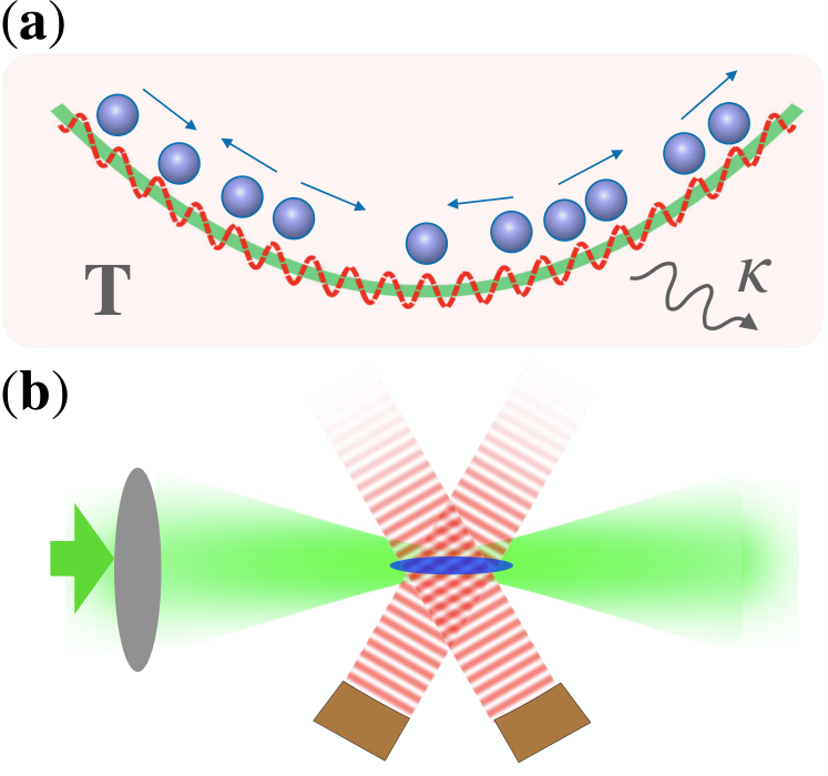
We consider the classical system of many particles trapped in a one-dimensional (1D) harmonic well and subjected to an additional periodically driven lattice potential with driving frequency as shown in Fig. 1(a). In the experiment, such model system can be realised with cold atoms in optical lattices Moritz et al. 2003 as shown in Fig. 1(b). At low temperature, the interaction of neutral cold atoms is dominated by -wave scattering process and can be modelled by an effective two-body contact potential Bloch et al. 2008. The total classical Hamiltonian of the system of atoms is given by
| (1) | |||||
where represents the single-atom Hamiltonian including the harmonic trap plus the driving potential, and represents the real-space interaction of two atoms. Here, all the variables have been scaled dimensionless by choosing the units of time, position and momentum as ( is the harmonic trapping frequency), (the characteristic length of driving lattice potential) and ( is the mass of particle) respectively. The unit of energy (Hamiltonian) is set to be .
In the open environment with dissipation rate (scaled by ) and temperature (scaled by with the Boltzmann constant), the classical EOM is given by
| (2) |
Here, the thermal noise term is introduced according to the fluctuation-dissipation relationship, where is the white noise satisfying
| (3) |
We now define the Wiener process as the integral of white noise, i.e., Using the property of white noise Eq. (3), one can show that
By further defining , we have
Therefore, we can write the EOM given by Eq. (2) as the following stochastic differential equation process
III Rotating frame
III.1 Hamiltonian within rotating wave approximation
We go to the rotating frame with frequency using the generating function of the second kind
Here, we have defined the ratio of driving frequency to harmonic frequency by and assumed the near-resonance condition with . Note that we can introduce some detuning between the driving and harmonic frequencies if , which will produce a parabolic confinement potential in phase space that is sometimes important to stabilise the phase space crystals Guo et al. 2022. The canonical transformation of coordinates is then given by , , i.e.,
The canonical transformation of Hamiltonian Eq. (1) in the rotating frame is given by
| (10) |
Due to the driving field and interaction of atoms, the quadratures of oscillation (amplitude and phase) are slowly moving. By plugging the transformation Eq. (III.1) into and neglecting all the time-dependent (fast oscillating) terms, we arrive at the effective static Hamiltonian in the rotating wave approximation (RWA)
| (11) |
We expect the RWA is valid when the driving field and the contact interaction strength between atoms are weak compared to the harmonic trapping frequency, which will be justified by our numerical simulation in Sec. III.3. Here, represents the RWA part of single-atom Hamiltonian , cf., Eq. (1).
For short-range interactions in real space, the effective RWA interaction becomes a function of the distance between atoms in phase space Guo et al. 2016; Guo and Liang 2020
| (12) |
This is because the atoms located at different phase space points will still collide in the course of their laboratory-frame trajectories. Thus, when we perform averaging of the Hamiltonian over time, the short-range interaction in the laboratory-frame gives rise to an effective long-range interaction in the rotating frame Sacha 2015b; Sacha 2015a; Guo et al. 2016; Giergiel et al. 2018b; Liang et al. 2018; Guo 2021. For the contact interaction of cold atoms in the laboratory frame, the effective interaction becomes long-range Coulomb-like interactionGuo et al. 2016; Liang et al. 2018; Guo 2021
| (13) |

III.2 Equations of motion within rotating wave approximation
For a closed system without dissipation, the canonical EOM under RWA in the rotating frame is given by
| (14) |
In order to obtain the EOM under RWA in the open environment with dissipation and thermal noise, we introduce the following transformation from Eq. (III.1)
By plugging Eq. (2) into Eq. (III.2), we have EOM including the dissipation and noise in the rotating frame
Here, we have defined the two orthogonal components of noises by
Obviously, we have and . From the relationship Eq. (3), we have the time correlation of two noise components as follows
| (23) | |||
| (24) | |||
| (25) |
Therefore, in the RWA (keeping only time-independent terms in the correlations), we can take and as independent standard white noises.
We plug Eq. (III.1) into EOM (III.2) and keep only static term in the spirit of RWA. Finally, we obtain the RWA EOM with dissipation and noise
As in Eq. (II), we introduce two independent Wiener processes for the two quadratures and and write the EOM (III.2) within RWA in the form of stochastic differential equation
III.3 Justification
In order to justify our RWA with dissipation and thermal noise, we consider the following classical many-body Hamiltonian with square phase space lattice described by
| (34) |
The square lattice of single-particle Hamiltonian in phase space can be generated by a kicking sequence of stroboscopic lattices (see details in Appendix)
| (35) |
Here, there are six kicks in each harmonic time period with kicking parameters , and . In fact, arbitrary lattice structures in phase space can be synthesized by properly choosing the kicking parameters Guo et al. 2022; Guo 2021.
The validity of RWA EOM without dissipation has been studied in the previous works Guo et al. 2016; Liang et al. 2018. Here, we justify our RWA EOM with finite dissipation rate and at finite temperature by comparing the prediction of Eqs. (III.2) with numerical solutions of the exact EOM (2). In our numerical simulation, we choose Lorenz function to model the contact interaction potential, i.e., . The corresponding phase space interaction potential is then given by Guo et al. 2016; Liang et al. 2018
| (36) |
In Fig. 2(a)-(b), we compare the dynamics of interacting particles obtained within RWA with the exact results obtained by solving Eqs. (II). We show 200 trajectories corresponding to 200 realizations of noise for the same initial conditions of the particles, and also present the averaged phase space variables . Clearly, the samples spread gradually as time evoluates. In Fig. 2(c), we plot the variance of threes particles in the phase space given by (cf. also Eqs. (61)-(62))
| (37) |
The numerical results show that the RWA approach agrees well with the exact dynamics. In fact, the RWA is valid when the dynamics of is much slower than the period of the harmonic oscillator potential.
IV Existence of phase space crystals
In the present section, we analyse the dynamics of phase space crystals based on the many-body dynamics and in the presence of dissipation and thermal noise and within the RWA, Eq. (III.2). Our goal is to identify the condition for the existence of phase space crystals. According to Eq. (12), the RWA interaction potential of two atoms depends on their relative distance in the phase space. Therefore, it is natural to extend the concept of force from configuration space to phase space. By defining the position vector in phase space and a unit direction vector perpendicular to the phase space plane , where and are the unit vectors in the position and momentum directions respectively, we can rewrite the EOM (III.2) in the following compact form
| (38) |
with the phase space force defined via
| (39) |
Here, we have defined the thermal noise vector
Based on the linear analysis of Eqs. (38) and (39), we will estimate the critical values of relevant parameters (dissipation rate, temperature and interaction strength) for the existence of phase space crystals, which will be verified by numerical simulations.
IV.1 Dissipation effects
For a closed system of particles without interaction, the fixed points are the extreme points determined by the condition We have with having the same parity. Finite values of dissipation rate, temperature and the presence of interaction will shift the fixed points and thus affect the existence of phase space crystals. We first consider the pure effects of dissipation at zero temperature () and without interaction (). In this case, the fixed points in phase space are given by the condition of . From Eq. (39), we have
| (40) |
where are the positions of the fixed points shifted by dissipation. We linearize Eq. (40) around the original fixed points as follows
| (41) |
where the Jacobian matrix and asymmetric tensor are given by
Solving Eq. (41), we get the shifted fixed points explicitly
The first term on the right hand side of Eq. (IV.1) is responsible for rotation of the whole lattice while the second term contracts the whole lattice along the radial direction.

If the shift of the fixed points is large enough, one can imagine that atoms will escape the lattice potential and the phase space crystals become “melting”. Since the displacement of the fixed points is proportional to their distance from the origin, cf. Eq. (IV.1), the crystal will start to melt from the edge. In order to calculate the critical dissipation rate where the atoms on the edge start to melt, we estimate the size of the final lattice limited due to dissipation. From Eq. (40), we have the following condition
| (49) | |||||
The above equation sets an upper limit for the lattice size condition, i.e. solutions for the fixed points exist if where . Considering the angular dependence of , we get a better empirical estimation for the radius of stable region from numerical simulations,
| (50) |
The area of stable region for the existence of phase space crystals is approximately
The total number of the fixed points inside the stable region is approximately
where is the density of atoms, e.g., one atom in each fixed point which corresponds to two atoms in each unit cell. If we assume that each fixed point is occupied by one atom, there is an upper limit for total atom number Given the number of atoms, the critical dissipation rate is
| (51) |
In Fig. 3, we show the initial state of atoms (left) and the final state due to the dissipation (right). The black dashed circle indicates the crystal radius predicted by Eq. (50). The dashed line indicates the rotation angle of the final lattice given by our predication, c.f. Eq (IV.1). Note that the two plots have the same number of atoms. As we do not consider interaction here, it is possible that more than one atoms occupy the same lattice site in the final crystal state.
IV.2 Temperature effects
We then study the effects of thermal noise that is determined by a finite temperature and dissipation rate , cf. Eq. (39). We apply linear approximation around the points to the EOM (38)
| (52) | |||||
We now define the following auxiliary vector
| (53) |
where is the shifted equilibrium point due to dissipation but at , cf., Eq. (41) or (IV.1). The vector is perpendicular to the displacement vector describing the shift . We simplify the stochastic differential equation (52) as follows
| (54) |
with
| (55) |
This stochastic differential equation describes a multi-dimensional Ornstein-Uhlenbeck process. The formal solution is given by
| (56) |
The mean value of stochastic process is
| (57) |
with
Here, P is the matrix diagonalising the matrix , i.e., .
For open dissipative environment, the eigenvalues and should be positive values such that in the long time limit. We further calculate the variance of as follows
| (61) | |||||
Here, we have used the property of white noise Eq. (3). Reminiscent of the definition of given by Eq. (55), it is not difficult to prove the following statement: If matrix is diagonal, we have the identities: , The Jacobian matrix, Eq. (IV.1), is indeed diagonal, , and thus holds in our case. Therefore, according to the Baker-Campbell-Hausdorff formula, we have
As a result, the variance of stochastic process given by Eq. (61) can be calculated explicitly as follows
| (62) | |||||
In Fig. 2(c), we compare the variance (62) with the results obtained by exact numerical simulations and within the RWA approach. Our analysis is based on the linear expansion around the stable points and it works well in short-time dynamics. The deviations grow gradually as the particle leaves further from the stable points,
Combining with Eq. (53), we have in the long-time limit , Therefore, the long-time distribution is a normal distribution with the width . In order to keep phase space crystal stable, we need the dispersion width much smaller than the characteristic length of unit cell (here we take )
| (63) |
In fact, the above relation can be directly obtained when we apply the equipartition theorem to the system in the laboratory frame. Considering a particle trapped at the bottom of harmonic well subjected to a both with temperature , the width of the thermal ground state is . Note that we have set the Boltzmann constant here. Actually, for any fixed point, in the regime where the temperature is so low that only slow motions are thermalized, we have
and thus , where is the average phase space position of a harmonic oscillator. The condition Eq. (63) just means that the phase space lattice constant (characteristic length of driving lattice) has to be much larger than the width of thermal state.

IV.3 Interaction effects
We now study the interaction effects on the existence of phase space crystals. For convenience, we separate the total Hamiltonian into the sum of two parts
| (64) | |||||
Here, we have introduced representing the summary of all single-particle square lattice Hamiltonians, and representing the sum of the interaction potentials. In the presence of the dissipation but at zero temperature , the fixed points are given by the condition , cf. Eq. (39),
| (65) |
where is the shifted fixed points to be calculated. By linearizing the above condition around the original fixed points satisfying , we obtain
| (66) | |||||
where and are Jacobian tensors defined by
Therefore, we have the shifted equilibrium points
It is straightforward to calculate tensor , cf., Eq. (IV.1). The difficulty is to calculate and . Below, we provide an approximate method to calculate them analytically.
For the Coulomb-like phase space interaction potential , cf., Eq. (13), the parameter plays the role of an effective charge. We assume that atoms are initially uniformly distributed in a disk shape with radius with density . We smear the point charges into a uniform charge distribution with charge density . Then, the interaction potential at the edge of the disk is given by
| (74) | |||||
Thus, the gradient of interacting potential at the edge is
| (75) |
where is the unit direction from the center of the disk to initial equilibrium position of -th atom, i.e., . Note that the phase space force given by Eq. (75) is only for the atoms at the edge and independent of the radius .
Using Eqs. (IV.1)-(IV.1) and (IV.3), we have the analytical expression for the shifted fixed point as follows
| (76) | |||||
Comparing to Eq. (IV.1), the interaction basically gives a correction to the effect of dissipation. The new equilibrium position is given by
| (77) | |||||
Following Eq. (49), we have the existence condition of phase space crystals with interaction
| (78) |
As in Eq. (49), by modifying the upper limit by and plugging Eq. (77) to Eq. (IV.3), we have the existence condition for stable phase space crystal state
| (79) |
By introducing the critical interaction strength and the critical dissipation rate as follows
| (80) |
where we have assumed that one atom is present per each fixed point, i.e. and , the existence condition (79) becomes
| (81) |
For large lattice , we have a simple condition
| (82) |
Although this condition for the existence of phase space crystals is obtained based on the linear analysis of dynamical system and other approximations, it provides a very good estimation for the phase transition as shown below by our numerical simulations. When the condition (82) breaks down, the atoms at the edge first escape their stable points and the entire crystal starts to melt from its edge, cf. Fig. 4(b).

IV.4 Phase diagram
To identify the existence of phase space crystal, we define the crystal order parameter as follows
| (83) |
In Fig. 4, we plot the crystal order parameter for different system parameters.
Let us first illustrate what happens with the crystal when there is no dissipation () but the interaction strength is larger than the critical value. In Fig. 4(a), we start from an initial state where atoms occupy the lattice sites in a finite disk-shape region. The corresponding crystal order parameter as a function of and is also shown in Fig. 4(a). For such perfect crystal state, the order parameter plot contains regular peaks that are periodically arranged in the -space, i.e., the positions of peaks appear at points with having the same parity. In Fig. 4(b), we plot the configuration of atoms in phase space and the crystal parameter in -space at time instant with . It is clearly shown that for the interaction strength and dissipation rate we consider here, the crystal starts to melt from the edge as predicted above, cf. Eq. (82) and the related discussion around. The corresponding crystal order parameter plot in the lower panel of Fig. 4(b) shows all the peaks diminish except the trivial peak at the center . In Fig. 4(c), we plot the configuration of atoms in phase space and the crystal parameter at time instant with . All the atoms escape from their equilibrium points and spread over the phase space forming a gas-like state in phase space. Because all the atoms are randomly distributed in phase space, all the nontrivial peaks in the crystal order parameter plot disappear.
Now, let us include the dissipation but at zero temperature. We choose the peak value of crystal order parameter at point to trace the phase diagram. Due to finite dissipation, the atoms need some time to relax to the final state. The characteristic relaxation time scale is of the order of . In Fig. 4(d), we plot the crystal order parameter for atoms as a function of the scaled interaction strength and the scaled dissipation rate . From the plots, it is clearly visible that there exists a region in the parameter space spanned by dissipation and interaction where the order parameter does not vanish. In Fig. 4(e), we plot the crystal order parameter as a function of the interaction strength for the dissipation rate and for five different atom numbers, i.e. . The sudden jump of the order parameter indicates a discontinuous phase transition. As the atom number increases with uniform density (approaching the scenario similar to thermodynamic limit in equilibrium state), the transition point approaches a fixed point close to (actually a bit lower than) our predicted value based on linear analysis, cf. the transition curves for and .
In order to show the effects of thermal noise on the formation of phase space crystals, we plot in Fig. 5 the crystal order parameter as a function of temperature for different dissipation rates and interaction strengths. We show the averaged value (connected points) and the standard deviation (coloured shadows) of the crystal order parameter obtained by simulating 200 different realizations of noise. At low temperature (), the order parameter is close to one indicating the existence of a crystal state in phase space. In contrast, at sufficiently high temperature, the order parameter is very close to zero indicating that the crystal state in phase space is totally dissolved. In each plot, we calculate the crystal order parameter for three different system sizes (atom numbers). As atom number increases, the plots approach a fixed curve corresponding to the thermodynamic limit. The standard deviation for each parameter set is zero at zero temperature (), and then starts to increase when the temperature increases. But as the temperature becomes high enough, the standard deviation goes back to zero again. This is because the phase space crystal state does not exist and the crystal order parameter vanishes for all realizations of noise we have simulated.
V Experimental Parameters
We now discuss whether the conditions for realizing classical phase space crystals can be satisfied in the real cold-atom experiments. We first examine the RWA condition that the driving strength , dissipation rate and interaction strength should be much smaller than unity in our units Guo et al. 2016; Liang et al. 2018. By recovering the units of parameters, we have the RWA condition
| (84) |
In the experiment of cold atoms Moritz et al. 2003, a quasi-1D harmonic potential with strong transverse trapping frequency is formed by propagating Gaussian laser beam(s). The resulting transverse trapping frequency and axial trapping frequency are given by , where is the Gaussian beam waist, () is the laser wavelength (wavenumber), is the intensity of lasers and is the recoil energy of an atom.
For the cold atoms () in the presence of the Gaussian laser with wavelength , beam waist and intensity , the transversal and axial trapping frequency are and respectively. By choosing the characteristic length of driving lattice potential (created by two additional laser beams, see Fig. 1) fifty times of the axial trapping length , we have the following RWA condition for driving strength
| (85) |
with the recoil energy . Therefore, we can tune the intensity of lasers that generate driving lattice potential to satisfy the RWA.
In the quasi-1D trap, the effective contact interaction is given by Bloch et al. 2008 where is the 3D -wave scattering length. Thus, we have the following RWA condition for interaction strength from Eq. (84)
| (86) |
Taking the 3D scattering length for atoms, we have the interaction strength satisfying RWA. The interaction strength can be further tuned either by transversal trapping frequency or by the Feshbach resonance Bloch et al. 2008.
Next, we estimate the critical parameters for the phase diagram in Fig. 4. According to Eq. (80), we have the critical driving strength and critical dissipation rate with recovered units
| (87) |
Using the driving strength and atom number , we have the critical values and . The dissipation rate (damping coefficient) for an atom can be tuned by the laser detuning from atomic frequency and set at resonance Metcalf and van der Straten 2007. Finally, to have stable phase space crystals, we need the temperature condition from Eq. (63)
| (88) |
which locates in the typical temperature range from the nanokelvin to the microkelvin regime in the cold-atom experiments Bloch et al. 2008.
VI Summary and Discussion
Many-body phase space crystal is an ordered highly excited state in a classical or quantum many-body dynamical system. Previous works on phase space crystals are restricted to closed system. In this work, we investigated the dynamics of classical many-body phase space crystals in the open dissipative environment with thermal noise. We started from the exact equations of motion of the system in the lab frame in the presence of dissipation and at non-zero temperature. We then derived and justified the equations of motion obtained within the rotating wave approximation in the rotating fame, which describes the slow dynamics of harmonic oscillation’s quadratures. We performed linear analysis of stability of the phase crystal and found that strong dissipation, interaction and high temperature can destroy the crystal state in phase space. We estimated the critical values of the parameters for the destruction of the phase space crystal. By defining a crystal order parameter, we plotted the phase diagram in the dissipation-interaction parameter plane and the order parameter as a function of temperature. The main conclusion is that phase space crystal state does exist for a range of parameter settings in the cold atom experiments.
In order to prepare such phase space crystals, one can initially set the cloud of atoms with driving, dissipation and interaction parameters below the critical values according to our prediction, but at relatively high temperature. In this scenario, the thermal noise will activate the atoms spreading over the phase space. Then, when cooling down the atoms, the finite dissipation will help the atoms to relax to the stable points nearby forming some blocks of phase space crystals. As the main goal of the present work is to prove the existence of phase space crystal state, we will study in detail how to prepare phase space crystals in the future work.
In this work, we have studied the square phase space crystalline structure for the single-particle Hamiltonian. An extension to other lattice structure like honeycomb lattice is straightforward. It has been shown that the phase space crystal vibrational band structure of honeycomb lattice can support chiral transport without breaking time-reversal symmetry Guo et al. 2022. Such kind of anomalous Chern insulator has not yet been realised in the experiments. We only investigated dynamics of phase space crystals in classical regime. The extended study in the quantum regime, which is closely related to (fractional) quantum Hall physics and 1D anyons Tosta et al. 2021; Greschner and Santos 2015, will be our future work.
Acknowledgements.
We acknowledge helpful discussions with Vittorio Peano and Florian Marquardt. Support of the National Science Centre, Poland, via Project No. 2018/31/B/ST2/00349 (A.E.K.) is acknowledged. This research was also funded in part by the National Science Centre, Poland, Project No. 2021/42/A/ST2/00017 (K.S.). For the purpose of Open Access, the author has applied a CC-BY public copyright licence to any Author Accepted Manuscript (AAM) version arising from this submission. Numerical computations in this work were supported in part by PL-Grid Infrastructure.Appendix A Square phase space lattice
To show how to generate the single-particle square phase space lattice in Eq. (34), we start from the following generalised model of a kicked harmonic oscillator
| (89) | |||||
where represents the kicking sequence of stroboscopic lattice with tunable intensity , wave vector and phase at different time instance with . To simplify the discussion, we first consider a single kicking sequence, i.e.,
| (90) | |||||
We transfer the above Hamiltonian into a rotating frame with the kicking frequency using the generating function of the second kind
which results in the transformation of phase space coordinates,
| (91) | |||||
| (92) |
and the transformed Hamiltonian
| (94) | |||||
Here, is the detuning between the kicking and harmonic oscillator frequencies. For weak resonant driving (), the single-particle dynamics can be simplified by averaging the Hamiltonian over the fast harmonic oscillations. The effective slow dynamics of quadratures is given by the lowest order Magnus expansion, i.e., the time average of over one kicking period,
Including all the kicks in Eq.(89), we obtain the general form of the phase space lattice Hamiltonian
In principle, any arbitrary lattice Hamiltonian in phase space can be synthesised by multiple stroboscopic lattices. For the square lattice considered in our work, we can get the desired driving parameters by decomposing the square lattice into a series of cosine functions, i.e.,
| (98) | |||||
| (100) | |||||
We decompose each term in the above equation as follows
| (101) | |||||
| (102) |
and
| (106) | |||||
| (110) | |||||
By comparing the above expansion to Eq. (A), we can generate the square phase space Hamiltonian by choosing the kicking parameters:
| (112) |
and and for all .
References
- Kubo (1957) Ryogo Kubo, “Statistical-mechanical theory of irreversible processes. i. general theory and simple applications to magnetic and conduction problems,” Journal of the Physical Society of Japan 12, 570–586 (1957).
- Onsager (1931) Lars Onsager, “Reciprocal relations in irreversible processes. i.” Phys. Rev. 37, 405–426 (1931).
- Prigogine (1945) Ilya Prigogine, “Modération et transformations irréversibles des systémes ouverts,” Bulletin de la Classe des Sciences, Académie Royale de Belgique. 31, 600–606 (1945).
- Prigogine (1978) Ilya Prigogine, “Time, structure, and fluctuations,” Science 201, 777–785 (1978).
- Haken (1983) H. Haken, “Advanced synergetics : Instability hierarchies of self-organizing systems and devices,” (Berlin New York: Springer-Verlag, 1983).
- Kuramoto and Nishikawa (1987) Yoshiki Kuramoto and Ikuko Nishikawa, “Statistical macrodynamics of large dynamical systems. case of a phase transition in oscillator communities,” Journal of Statistical Physics 49, 569–605 (1987).
- May (1976) Robert M. May, “Simple mathematical models with very complicated dynamics,” Nature 261, 459–467 (1976).
- Lorenz (1963) Edward N. Lorenz, “Deterministic nonperiodic flow,” Journal of Atmospheric Sciences 20, 130 – 141 (1963).
- Nicolis and Prigogine (1977) G. Nicolis and I. Prigogine, “Self-organization in nonequilibrium systems: From dissipative structures to order through fluctuations,” (Wiley, New York, 1977).
- Getling (1998) A V Getling, “Rayleigh-bénard convection,” (WORLD SCIENTIFIC, 1998).
- Hudson and Mankin (1981) J. L. Hudson and J. C. Mankin, “Chaos in the belousov?zhabotinskii reaction,” The Journal of Chemical Physics 74, 6171–6177 (1981).
- Lee and Sadeghpour (2013) Tony E. Lee and H. R. Sadeghpour, “Quantum synchronization of quantum van der pol oscillators with trapped ions,” Phys. Rev. Lett. 111, 234101 (2013).
- Lörch et al. (2017) Niels Lörch, Simon E. Nigg, Andreas Nunnenkamp, Rakesh P. Tiwari, and Christoph Bruder, “Quantum synchronization blockade: Energy quantization hinders synchronization of identical oscillators,” Phys. Rev. Lett. 118, 243602 (2017).
- Weiss et al. (2017) Talitha Weiss, Stefan Walter, and Florian Marquardt, “Quantum-coherent phase oscillations in synchronization,” Phys. Rev. A 95, 041802(R) (2017).
- Thomas and Senthilvelan (2022) Nissi Thomas and M. Senthilvelan, “Quantum synchronization in quadratically coupled quantum van der pol oscillators,” Phys. Rev. A 106, 012422 (2022).
- Svensson et al. (2017) Ida-Maria Svensson, Andreas Bengtsson, Philip Krantz, Jonas Bylander, Vitaly Shumeiko, and Per Delsing, “Period-tripling subharmonic oscillations in a driven superconducting resonator,” Phys. Rev. B 96, 174503 (2017).
- Svensson et al. (2018) Ida-Maria Svensson, Andreas Bengtsson, Jonas Bylander, Vitaly Shumeiko, and Per Delsing, “Period multiplication in a parametrically driven superconducting resonator,” Applied Physics Letters 113, 022602 (2018).
- Arndt and Hassler (2022) Lisa Arndt and Fabian Hassler, “Period tripling due to josephson parametric down-conversion beyond the rotating-wave approximation,” Phys. Rev. B 106, 014513 (2022).
- Lazarides et al. (2014) Achilleas Lazarides, Arnab Das, and Roderich Moessner, “Equilibrium states of generic quantum systems subject to periodic driving,” Phys. Rev. E 90, 012110 (2014).
- D’Alessio and Rigol (2014) Luca D’Alessio and Marcos Rigol, “Long-time behavior of isolated periodically driven interacting lattice systems,” Phys. Rev. X 4, 041048 (2014).
- Ponte et al. (2015) Pedro Ponte, Anushya Chandran, Z. Papić, and Dmitry A. Abanin, “Periodically driven ergodic and many-body localized quantum systems,” Annals of Physics 353, 196–204 (2015).
- Sacha and Zakrzewski (2017) Krzysztof Sacha and Jakub Zakrzewski, “Time crystals: a review,” Reports on Progress in Physics 81, 016401 (2017).
- Khemani et al. (2019) Vedika Khemani, Roderich Moessner, and S. L. Sondhi, “A brief history of time crystals,” (2019).
- Else et al. (2020) Dominic V. Else, Christopher Monroe, Chetan Nayak, and Norman Y. Yao, “Discrete time crystals,” Annual Review of Condensed Matter Physics 11, 467–499 (2020).
- Guo and Liang (2020) Lingzhen Guo and Pengfei Liang, “Condensed matter physics in time crystals,” New Journal of Physics 22, 075003 (2020).
- Khemani et al. (2016) Vedika Khemani, Achilleas Lazarides, Roderich Moessner, and S. L. Sondhi, “Phase structure of driven quantum systems,” Phys. Rev. Lett. 116, 250401 (2016).
- Else et al. (2016) Dominic V. Else, Bela Bauer, and Chetan Nayak, “Floquet time crystals,” Phys. Rev. Lett. 117, 090402 (2016).
- Yao et al. (2017) N. Y. Yao, A. C. Potter, I.-D. Potirniche, and A. Vishwanath, “Discrete time crystals: Rigidity, criticality, and realizations,” Phys. Rev. Lett. 118, 030401 (2017).
- Sacha (2015a) Krzysztof Sacha, “Modeling spontaneous breaking of time-translation symmetry,” Phys. Rev. A 91, 033617 (2015a).
- Russomanno et al. (2017) Angelo Russomanno, Fernando Iemini, Marcello Dalmonte, and Rosario Fazio, “Floquet time crystal in the lipkin-meshkov-glick model,” Phys. Rev. B 95, 214307 (2017).
- Giergiel et al. (2018a) Krzysztof Giergiel, Arkadiusz Kosior, Peter Hannaford, and Krzysztof Sacha, “Time crystals: Analysis of experimental conditions,” Phys. Rev. A 98, 013613 (2018a).
- Matus and Sacha (2019) Paweł Matus and Krzysztof Sacha, “Fractional time crystals,” Phys. Rev. A 99, 033626 (2019).
- Giergiel et al. (2019) Krzysztof Giergiel, Arkadiusz Kuroś, and Krzysztof Sacha, “Discrete time quasicrystals,” Phys. Rev. B 99, 220303(R) (2019).
- Mori et al. (2016) Takashi Mori, Tomotaka Kuwahara, and Keiji Saito, “Rigorous bound on energy absorption and generic relaxation in periodically driven quantum systems,” Phys. Rev. Lett. 116, 120401 (2016).
- Kuwahara et al. (2016) Tomotaka Kuwahara, Takashi Mori, and Keiji Saito, “Floquet-magnus theory and generic transient dynamics in periodically driven many-body quantum systems,” Annals of Physics 367, 96–124 (2016).
- Abanin et al. (2015) Dmitry A. Abanin, Wojciech De Roeck, and Fran çois Huveneers, “Exponentially slow heating in periodically driven many-body systems,” Phys. Rev. Lett. 115, 256803 (2015).
- Kim et al. (2006) Kihwan Kim, Myoung-Sun Heo, Ki-Hwan Lee, Kiyoub Jang, Heung-Ryoul Noh, Doochul Kim, and Wonho Jhe, “Spontaneous symmetry breaking of population in a nonadiabatically driven atomic trap: An ising-class phase transition,” Phys. Rev. Lett. 96, 150601 (2006).
- Heo et al. (2010) Myoung-Sun Heo, Yonghee Kim, Kihwan Kim, Geol Moon, Junhyun Lee, Heung-Ryoul Noh, M. I. Dykman, and Wonho Jhe, “Ideal mean-field transition in a modulated cold atom system,” Phys. Rev. E 82, 031134 (2010).
- Luitz et al. (2020) David J. Luitz, Roderich Moessner, S. L. Sondhi, and Vedika Khemani, “Prethermalization without temperature,” Phys. Rev. X 10, 021046 (2020).
- Else et al. (2017) Dominic V. Else, Bela Bauer, and Chetan Nayak, “Prethermal phases of matter protected by time-translation symmetry,” Phys. Rev. X 7, 011026 (2017).
- Autti et al. (2021) S. Autti, P. J. Heikkinen, J. T. Mäkinen, G. E. Volovik, V. V. Zavjalov, and V. B. Eltsov, “Ac josephson effect between two superfluid time crystals,” Nature Materials 20, 171–17 (2021).
- Hannaford and Sacha (2022a) Peter Hannaford and Krzysztof Sacha, “Condensed matter physics in big discrete time crystals,” AAPPS Bulletin 32, 12 (2022a).
- Giergiel et al. (2018b) Krzysztof Giergiel, Artur Miroszewski, and Krzysztof Sacha, “Time crystal platform: From quasicrystal structures in time to systems with exotic interactions,” Phys. Rev. Lett. 120, 140401 (2018b).
- Giergiel et al. (2020) Krzysztof Giergiel, Tien Tran, Ali Zaheer, Arpana Singh, Andrei Sidorov, Krzysztof Sacha, and Peter Hannaford, “Creating big time crystals with ultracold atoms,” New Journal of Physics 22, 085004 (2020).
- Kuroś et al. (2020) Arkadiusz Kuroś, Rick Mukherjee, Weronika Golletz, Frederic Sauvage, Krzysztof Giergiel, Florian Mintert, and Krzysztof Sacha, “Phase diagram and optimal control for n-tupling discrete time crystal,” New Journal of Physics 22, 095001 (2020).
- Giergiel et al. (2021) Krzysztof Giergiel, Arkadiusz Kuroś, Arkadiusz Kosior, and Krzysztof Sacha, “Inseparable time-crystal geometries on the möbius strip,” Phys. Rev. Lett. 127, 263003 (2021).
- Matus et al. (2021) Paweł Matus, Krzysztof Giergiel, and Krzysztof Sacha, “Anderson complexes: Bound states of atoms due to anderson localization,” Phys. Rev. A 103, 023320 (2021).
- Hannaford and Sacha (2022b) Peter Hannaford and Krzysztof Sacha, “A decade of time crystals: Quo vadis?” Europhysics Letters 139, 10001 (2022b).
- Golletz et al. (2022) Weronika Golletz, Andrzej Czarnecki, Krzysztof Sacha, and Arkadiusz Kuroś, “Basis for time crystal phenomena in ultra-cold atoms bouncing on an oscillating mirror,” New Journal of Physics 24, 093002 (2022).
- Kopaei et al. (2022) Ali Emami Kopaei, Xuedong Tian, Krzysztof Giergiel, and Krzysztof Sacha, “Topological molecules and topological localization of a rydberg electron on a classical orbit,” Phys. Rev. A 106, L031301 (2022).
- Guo (2021) Lingzhen Guo, Phase Space Crystals, 2053-2563 (IOP Publishing, 2021).
- Sacha (2020) Krzysztof Sacha, “Phase space crystals,” in Time Crystals (Springer International Publishing, Cham, 2020) pp. 237–249.
- Guo et al. (2013) Lingzhen Guo, Michael Marthaler, and Gerd Schön, “Phase space crystals: A new way to create a quasienergy band structure,” Phys. Rev. Lett. 111, 205303 (2013).
- Lang and Armour (2021) Ben Lang and Andrew D Armour, “Multi-photon resonances in josephson junction-cavity circuits,” New Journal of Physics 23, 033021 (2021).
- Liang et al. (2018) Pengfei Liang, Michael Marthaler, and Lingzhen Guo, “Floquet many-body engineering: topology and many-body physics in phase space lattices,” New Journal of Physics 20, 023043 (2018).
- Guo et al. (2022) Lingzhen Guo, Vittorio Peano, and Florian Marquardt, “Phase space crystal vibrations: Chiral edge states with preserved time-reversal symmetry,” Phys. Rev. B 105, 094301 (2022).
- Bloch et al. (2008) Immanuel Bloch, Jean Dalibard, and Wilhelm Zwerger, “Many-body physics with ultracold gases,” Rev. Mod. Phys. 80, 885–964 (2008).
- Hadzibabic et al. (2004) Zoran Hadzibabic, Sabine Stock, Baptiste Battelier, Vincent Bretin, and Jean Dalibard, “Interference of an array of independent bose-einstein condensates,” Phys. Rev. Lett. 93, 180403 (2004).
- Moritz et al. (2003) Henning Moritz, Thilo Stöferle, Michael Köhl, and Tilman Esslinger, “Exciting collective oscillations in a trapped 1d gas,” Phys. Rev. Lett. 91, 250402 (2003).
- Guo et al. (2016) Lingzhen Guo, Modan Liu, and Michael Marthaler, “Effective long-distance interaction from short-distance interaction in a periodically driven one-dimensional classical system,” Phys. Rev. A 93, 053616 (2016).
- Sacha (2015b) Krzysztof Sacha, “Anderson localization and mott insulator phase in the time domain,” Scientific Reports 5, 10787 (2015b).
- Metcalf and van der Straten (2007) Harold J. Metcalf and Peter van der Straten, “Laser cooling and trapping of neutral atoms,” in The Optics Encyclopedia (John Wiley & Sons, Ltd, 2007).
- Tosta et al. (2021) Allan D. C. Tosta, Ernesto F. Galvão, and Daniel J. Brod, “Gaussian optical networks for one-dimensional anyons,” Phys. Rev. A 104, 022604 (2021).
- Greschner and Santos (2015) Sebastian Greschner and Luis Santos, “Anyon hubbard model in one-dimensional optical lattices,” Phys. Rev. Lett. 115, 053002 (2015).