Differentially rotating scalarized neutron stars with realistic post-merger profile
Abstract
The merger remnant of a binary neutron star coalescence is initially strongly differentially rotating. Some properties of these remnants can be accurately modeled through building equilibrium neutron star models. In the present paper, we study how a modification of general relativity, namely scalar-tensor theory with a massive scalar field, will alter the picture. In contrast to previous studies, we implement a realistic phenomenological differential rotational law which allows for neutron star models to attain maximal angular velocity away from the center. We find that solutions with much higher masses and angular momenta exist in scalar-tensor theory compared to general relativity. They keep their quasi-spherical energy-density distribution for significantly higher values of the angular momentum before transitioning to quasi-toroidal models, in contrast to pure general relativity. Constructing such neutron star solutions is the first step to our final goal that is studying how scalarization alters the stability and gravitational wave emission of post-merger remnants.
I Introduction
Gravitational waves observations and the prospect for multimessenger astronomy gives us the tools to study nature’s laws in their extreme. Among the best candidates are neutron star (NS) merger events, such as GW170817 Abbott et al. 2017a; Abbott et al. 2017b, that allow us to study the behaviour of matter in the condition of extreme density and strong gravity. For that purpose, mergers of binary NSs have been modelled in general relativity (GR) with fully nonlinear three-dimensional simulations, see e.g. Hotokezaka et al. 2011; Sekiguchi et al. 2011; Bauswein and Janka 2012; Hotokezaka et al. 2013; Bernuzzi et al. 2014; Dietrich et al. 2015; Radice et al. 2018; De Pietri et al. 2018. Since one of the main goals of gravitational wave observations is to test gravity in the realm of strong gravitational fields (see e.g. Yunes and Siemens 2013; Berti et al. 2015; Abbott et al. 2019; Abbott et al. 2021; Arun et al. 2022 and references therein), a natural extension of these results is to include modified gravity effects. Even in the scope of pure GR, though, merger simulations are very challenging and computationally demanding. Hence, extending them for modified theories of gravity is a highly nontrivial task and has been done only in a handful of cases Barausse et al. 2013; Shibata et al. 2014; East and Pretorius 2022; Sagunski et al. 2018; Bezares et al. 2021. If one concentrates only on studying certain properties of the merger remnant, though, the problem can be simplified considerably. Assuming that after the merger a neutron star is formed instead of a direct collapse to a black hole, it will be initially strongly differentially rotating. It is possible to construct axisymmetric equilibrium models of such differentially rotating NSs, with properties that resemble those of merger remnants Camelio et al. 2019; Camelio et al. 2021; Iosif and Stergioulas 2021; Iosif and Stergioulas 2022. Such equilibrium models can serve as a tool to gain important insight into the post-merger dynamics, as detailed below.
In order for this to be done, a realistic differential rotation law, which can reproduce the merger remnant rotational profile, is needed. The well-know and widely used -constant differential rotation law Komatsu et al. 1989 is very useful to gain a first insight in the problem and helped understand the phenomenology. It was found that different types of differentially rotating models can exist, including the quasi-toroidal (the co-called type C), the quasi-spherical (type A) and some additional, more exotic types, see Ansorg et al. 2009; Espino and Paschalidis 2019; Bozzola et al. 2019. The stability of such models was examined through numerical simulations, e.g. in Duez et al. 2006; Giacomazzo et al. 2011; Weih et al. 2018; Espino et al. 2019; Szewczyk et al. 2023.
The -constant law can not model accurately, though, the post-merger remnant. Perhaps the simplest extension that performs better is the 3-parameter law considered in Bauswein and Stergioulas 2017; Bozzola et al. 2018. A more realistic improvement was developed by Uryu et al. in Uryu et al. 2017; Uryu et al. 2017 where a four-parameter differential rotation law was proposed, which allows a neutron star model to attain maximal angular velocity away from the center, a generic property of post-merger remnants seen in all simulations. In Iosif and Stergioulas 2021; Iosif and Stergioulas 2022 the authors constructed equilibrium sequences of differentially rotating relativistic stars employing this four-parameter rotation law Uryu et al. 2017, with parameters motivated by simulations of binary merger remnants. Both polytropic and realistic equations of state (EoS) were considered and both quasi-spherical (type A) and quasi-toroidal (type C) models were constructed.
The quasi-equilibrium models of post-merger remnants can have a variety of applications. This includes the interpretation of the post-merger gravitational wave (GW) spectrum Bauswein and Janka 2012; Takami et al. 2015, the study of the threshold mass to prompt collapse to a black hole Bauswein and Stergioulas 2017; Rezzolla et al. 2018; Shibata et al. 2019, the modeling of processes taking place on longer secular timescales that can not be easily addressed with nonlinear simulations Doneva et al. 2015, etc. Most of the studies on this topic, though, are performed in pure GR. Modification of the theory of gravity can significantly influence the neutron star equilibrium and the gravitational wave emission in dynamical processes (e.g. Blázquez-Salcedo et al. 2019; Blázquez-Salcedo et al. 2022). An example are the scalar-tensor theories (STT), that are among the most natural and widely studied modification of GR, where the additional scalar field can lead to considerable increase of the stellar maximum mass, especially in the case of rapid rotation Damour and Esposito-Farese 1993; Doneva et al. 2013; Doneva and Yazadjiev 2016. The quasinormal mode spectrum can be significantly altered as well, e.g. Sotani and Kokkotas 2004; Blázquez-Salcedo et al. 2020; Krüger and Doneva 2021 and new types of oscillations can appear, e.g. Mendes et al. 2021. All this hints towards the idea that the predictions mentioned above in GR might change significantly in the presence of additional fields. Thus, the gravitational wave observations will allow us to put strong constraints on modified gravity.
The study of quasi-equilibrium rotating post-merger models in modified gravity is a practically undeveloped area. As a matter of fact, there are just a handful of papers constructing uniformly rotating neutron stars in modified gravity Doneva et al. 2013; Kleihaus et al. 2014; Doneva and Yazadjiev 2016; Kleihaus et al. 2016, while differential rotation was considered only in Doneva et al. 2018. The differential rotation law employed in the latter paper was the simplified -constant law that can not model well post-merger remnants. It still demonstrated, though, how different post-merger quasi-equilibrium models can differ from GR (for results from fully nonlinear dynamical merger simulations in modified gravity see Shibata et al. 2014). This motivates us to extend on the above-mentioned papers and study differentially rotating models in scalar-tensor theory with the realistic four-parameter rotation law of Uryu et al. 2017, which attains maximal angular velocity away from the center. These models can be used as a background for studying stability and gravitational wave emission that will be done in a follow-up paper.
Another extension to Doneva et al. 2018 is that we consider the cases of nonzero scalar field mass. Apart from the fact that this is an interesting generalization of the model, the scalar field mass has another very important role – to help us evade the binary pulsar observation that for the moment have ruled out completely scalarization in the classical scalar-tensor theories with zero scalar field potential Zhao et al. 2022. This property comes from the fact that for a nonzero scalar field mass the scalar field has a finite range of the order of its Compton wavelength. Thus, if this Compton wavelength is below the binary pulsar separation, the two orbiting compact objects would not feel each other’s field Ramazanoğlu and Pretorius 2016; Yazadjiev et al. 2016. A scalar field mass as small as eV is sufficient to evade all binary pulsar constraints while leaving the equilibrium compact object models and their dynamics almost indistinguishable from the massless scalar field case11 1 The effect of the scalar field mass starts to be well pronounced in the neutron star structure and dynamics only for a few orders of magnitude larger mass than eV..
The structure of this paper is as follows: in Section II we briefly present the mathematical background for the considered STT and for the differential rotation. In Section III we present the numerical results. The paper ends with a Conclusion.
II Scalar-tensor theory and differential rotation low
The general form of the Einstein frame action for scalar-tensor theories is
| (1) |
where is the Ricci scalar with respect to the Einstein frame metric , is the scalar field potential and is the Einstein frame coupling function between the matter and the scalar field that appears in the action of the matter . The matter fields are collectively denoted by . The field equations obtained after varying the action above have the form
| (2) | |||||
| (3) |
where is the coupling function defined as
| (4) |
In the present paper we will consider theory with massive scalar field with potential
| (5) |
and coupling function
| (6) |
where and are constants. The case of and corresponds to the famous Brans-Dicke theory while for and we have the Damour-Esposito-Farese model allowing for neutron star scalarization Damour and Esposito-Farese 1993. Interestingly, when the radial perturbations of a compact object also lead to gravitational wave emission related with the presence of the so-called breathing polarisation modes.
The idea behind introducing a scalar field potential is not only to explore possible modifications beyond GR in their full richness. As discussed in the introduction, even more important is that even a very small , that practically has a negligible effect on the structure of compact objects, can evade the binary pulsar constraints Zhao et al. 2022 and allow for larger deviations from GR in the strong field regime.
We consider stationary and axisymmetric matter and scalar field configurations that allow us to use the following form of the metric:
| (7) |
where all metric functions depend only on and . The explicit form of the dimensionally reduced field equations is quite lengthy and that is why we refer the interested reader to Doneva et al. 2013; Doneva and Yazadjiev 2016; Yazadjiev et al. 2015.
Having discussed the metric and the scalar field, let us focus now on how the matter is treated. The conservation of the energy-momentum tensor in the Einstein frame takes the following form
| (8) |
We will assume that the NS are made out of a perfect fluid with an energy-momentum tensor being
| (9) |
where and are the pressure and energy density of the fluid. The Einstein frame fluid four velocity takes the form
| (10) |
where is the angular velocity and the proper velocity of the fluid is given by . In the differentially rotating case we study here , while for uniform rotation the angular velocity is a constant.
The quantities defined so far are in the for computations more convenient Einstein frame. The final results presented in this paper, however, are transformed back in the physical Jordan frame. The two frames are related by a conformal transformation and a redefinition of the scalar field. The interested reader can find the detailed relations between the two frames in Doneva et al. 2013. Here, we will only mention some of the relations we need for the presentation of the results in the paper.
The energy-momentum tensor, the energy density, the pressure and the four velocity transform between the two frames as
| (11) | |||||
where the Jordan frame quantities are denoted with a tilde. and remain the same in both frames. Let us comment on the relation between the Jordan and the Einstein frame mass, radius and angular momentum of the star. The tensor mass of the neutron stars is by definition the ADM mass in the Einstein frame and this mass coincides with the Jordan frame one for the considered coupling function (6). The angular momentum is by definition the same in both frames as well. The circumferential radius of the star, though, differs and the physical Jordan frame stellar radius is
| (12) |
where is defined to be the Einstein frame coordinate equatorial radius of the star. by itself is defined as the location where the pressure vanishes .
The field equations and the equation for hydrostationary equilibrium should be supplemented with an EoS. The equation of state, however, is given in the physical Jordan frame, hence it is more convenient to use and for the rest of the section. With the above assumptions and notations, the hydrostationary equilibrium equation has the following explicit form
| (13) |
In the preset paper we will use a realistic four parameter differential rotation law Uryu et al. 2017
| (14) |
where is the gravitationally redshifted angular momentum per unit rest mass and enthalpy, while and are constants. When implementing this differential rotation law we will follow the procedure developed GR in Iosif and Stergioulas 2021 taking into account the needed modification related to the addition of a scalar field. The two of the free parameters should be fixed to and , which allows the equation for hydrostationary equilibrium to be cast in a simpler form required by the RNS code Uryu et al. 2017; Iosif and Stergioulas 2021. Instead of directly using the other two parameters and , though, we introduce new parameters and which are given as relations between the angular velocity at the center of the star , the angular velocity at the equator , and the maximal angular velocity in the following way
| (15) | |||
| (16) |
When one sets values for and and substitute the rotational law (14) in the above relations, the obtained system is solved for and at each iteration. The motivation behind the use of and roots in the fact that it is easier to reproduce the Newtonian limit Uryu et al. 2017 and it is more convenient for controlling the type of differentially rotating model, e.g. whether it is quasi-toroidal or quasi-spherical. This problem is discussed in greater detail in Iosif and Stergioulas 2021 and we refer the interested reader to this paper for further information.
III Numerical results
The main goal of the present paper is to study the effect of the scalar-tensor theory on differentially rotating equilibrium neutron stars that can serve as a model of post-merger remnants with the more realistic four-parameter differential rotation law (14). Hence, it would be enough to concentrate on a single realistic cold equation of state and we have chosen the MPA1 EOS Müther et al. 1987. Even with the single EoS, and fixing and in (14), we are left with five free parameters, namely three connected to the STT (, , ), and two connected with the differential rotation (, ). Since the focus of the paper is on the modified gravity effects, and in order to keep the outline consize, we have decided to fix and and concentrate on the effect of changing the STT parameters (, , ). The exploration of the former parameters, especially in connection to actual merger simulation in STT, will be done in a follow-up publication.
We will focus on a combination of (, ) that leads to quasi-toroidal models in GR. In STT, though, the quasi-toroidal energy-density distribution appears only for extremely large angular momenta. The simulations of binary neutron star remnants, on the other hand, show that such quasi-toroidal models are a transient phase appearing right after the merger. Shortly afterwards, the remnants settle into type A, quasi-spherical, models. Thus the fact that producing a quasi-toroidal model in the presence of a strong enough scalar field is possible only in a very limited region of the parameter space, can have interesting astrophysical consequences.
Based on previous studies in GR Iosif and Stergioulas 2021; Iosif and Stergioulas 2022 we have chosen to work with . For the numerical calculations we developed a modification of the RNS code Stergioulas and Friedman 1995; Doneva et al. 2018. All quantities presented in this section are in the physical Jordan frame.
III.1 General properties for sequences of diffentially rotating neutron stars
As a first step in our study we concentrate on the global properties of the differentially rotating models in STT, and how the parameters of the theory and the mass of the field effect them. For that purpose it will be most suitable to examine sequences of models with constant angular momentum (in dimensionless units ) similar to the studies in GR Iosif and Stergioulas 2021; Iosif and Stergioulas 2022 since this is one of the conserved quantities. In Fig. 1 we present the mass of the star as a function of the maximal energy density in the left panel and as a function of the equatorial radius in the right panel. The presented sequences of models are for GR and massless STT with some representative values of the parameters , and . As we will see below, these results are practically indistinguishable from the case of eV that is roughly the minimum one allowing to safely evade binary pulsar observations.
Let us first focus on the nonrotating case with . Strictly speaking, for all models are endowed with scalar field. Thus, GR is not a solution of the field equations and spontaneous scalarization in the sense of Damour and Esposito-Farese 1993 is not possible. For the chosen parameters in the STT, though, we observe a scenario which closely resembles scalarization. For low compactness the GR and the STT branches practically overlap since the scalar field is negligible. After a certain critical compactness is reached the scalar field sharply increases that resembles the onset of scalarization and the first bifurcation-like point is formed. This scalarized branch reaches a maximum mass and afterwards the scalar field decreases again to very small value and practically merges again with the GR one at a second bifurcation-like point.
After discussing the sequences let us move to larger in Fig. 1. In the figure we start with (in geometrical units) that corresponds already to a very fast rotation. As seen, we could not obtain the first bifurcation-like point numerically but at least the scalarized sequence have a well pronounced shape with a maximum and second bifurcation-like point appearing. With the increase of the sequences get increasingly short and for very large we could obtain only a small part of the neutron star sequence, both for GR and STT. The problem of generating longer sequences of solutions is numerical as discussed in detail in Iosif and Stergioulas 2021; Iosif and Stergioulas 2022, namely the modified RNS code fails to converge to a unique solution. Nevertheless, we invested a lot of efforts in obtaining long enough sequences of deferentially rotating neutron stars so that we can judge about the new physics induced by the presence of a scalar field.
The first important observation is that in GR we were able to find solutions with up to roughly as seen in Fig. 1. In STT with and , however, the situation is dramatically different and solutions with much higher exist. We managed to reach up to roughly but we have indications that higher might be also possible. Similar indications for larger sequences in STT were already observed for neutron stars with -constant differential rotation law Doneva et al. 2018 but the maximum that was reached there was much smaller. As expected, with the increase of , we observe significant increase of the neutron star mass. Such high models can have very interesting astrophysical implications for the post-merger evolution that will be discussed in the conclusions.
In Fig. 2 we focus on the behavior of the solutions with varying theory parameters (). In the left panel we present the mass of the star as a function of its radius for fixed and varying (again for ). The chosen value of is relatively small (in absolute value) in order to demonstrate better the effect of . The presented models are with two fixed angular momenta for which both GR and scalarized solutions could be found, namely and . As expected, the increase of leads to a stronger scalar field and thus deviations from GR but the qualitative picture remains similar. The only major difference is that for larger enough there are no bifurcation-like points anymore and the neutron star solutions always deviate non-negligibly from GR.
The right panel of Fig. 2 serves as a proof of the conjecture expressed above, namely that a small scalar field mass that can evade binary pulsar experiments, have no measurable influence on the neutron star structure with respect to the massless case. In order to demonstrate that we present the mass of the star as a function of its radius for fixed and , and two masses, and eV. As seen, there is no visible difference between the massive and the massless case. This justifies the fact that for simplicity and convenience from a numerical point of view, a big portion of our results are presented for .
III.2 Profiles of scalarized differentially rotating neutron stars
We continue our study of differentially rotating scalarized neutron stars by examining individual models. In Fig. 3 we compare the surface profiles of the stars, plotted in the plane (both coordinates are normalized to the equatorial coordinate radius ) (top row) and the angular velocity distributions in the equatorial plane as a function of the circumferential radial coordinate , normalized to the circumferential radius of the star (bottom row). All models have fixed baryon mass and two different values of the angular momentum, namely and . The parameter is fixed to and two different values for are presented. As one can see, for the same , the GR models are the most toroidal ones while with the decrease of and thus the increase of the scalar field strength, the toroidal shape is softened. As a general observation we can say that in the STT, the differentially rotating models stay spherical (or quasi-spherical) for much higher values of (even beyond those allowed in GR). This was also observed for differentially rotating models with -constant law Doneva et al. 2018. Concerning the angular velocity, in the GR case it is the highest and it decreases with the decrease of .
In Fig. 4 we study the effect of the scalar field mass on individual models as well as the effect of extremely high for which only scalarized solutions exist. Thus, we present two values of , namely and , and several scalar field masses, while and are kept fixed. The models we study are with fixed maximal energy-density . The reason is that this is more convenient than a fixed baryon mass in the case of high where neutron star solutions exist in a much more narrow range of parameters. As one can expect, based on the known results for massive STT Yazadjiev et al. 2016; Doneva and Yazadjiev 2016, the increase of the scalar field mass suppresses the effect of scalarization and the results converge to the GR case (if it exist) as the mass of the field goes to infinity. Therefore, the models get more toroidal with the increase of and the angular velocity increases as well as seen in Fig. 4. For all considered combinations of and , though, the toroidal deformation remains still moderate in comparison with GR.
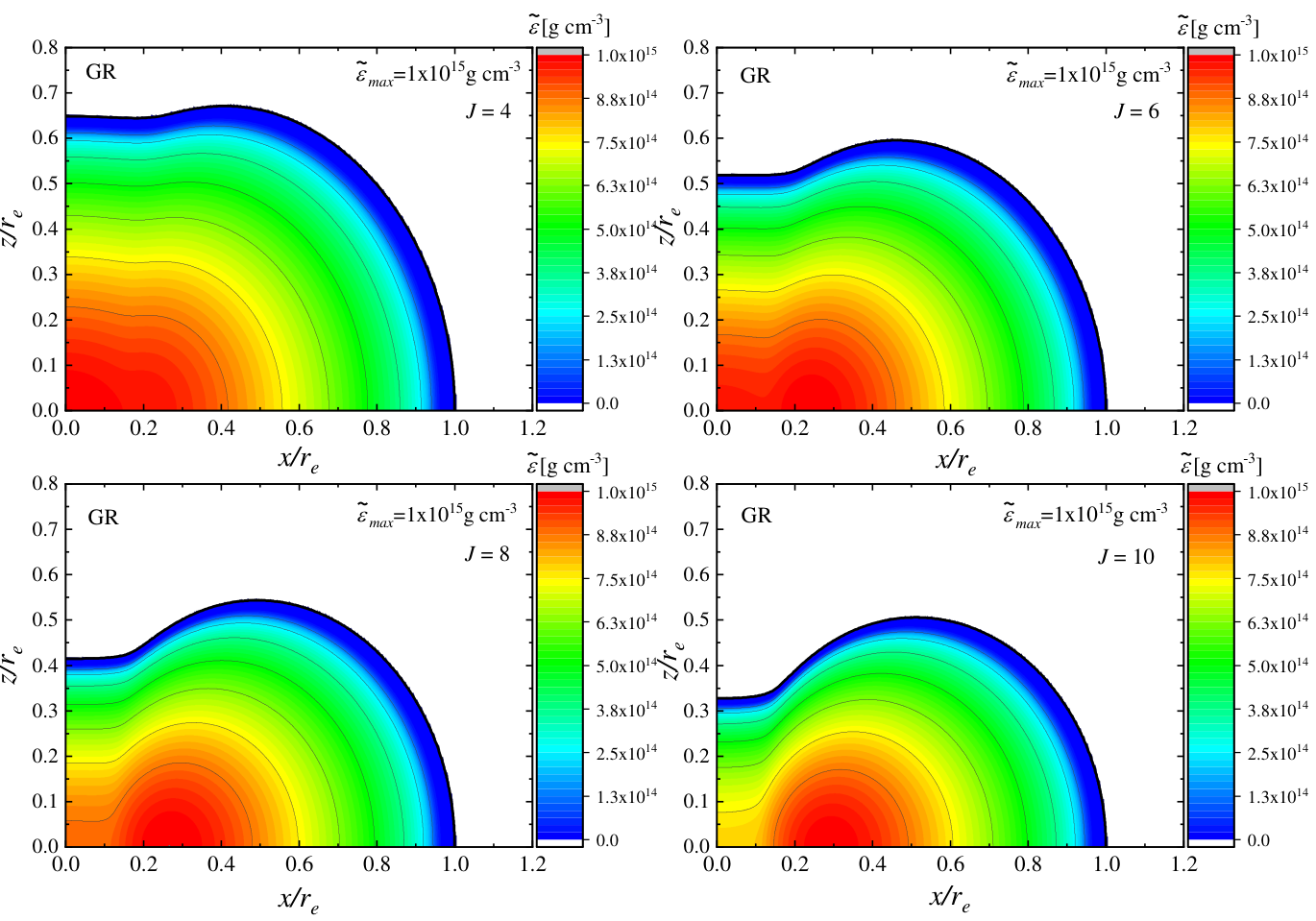
The reason why we observe less-toroidal profiles for larger absolute values of lies in the geometry of the scalar field. As already observed even for uniformly rotating models Doneva et al. 2013, despite the larger deformation of the neutron star fluid shape away from a sphere in the case of very rapid (differential) rotation, the geometry of the scalar field remains nearly spherical. In order to better understand the effect of the scalar field in our case, we proceed with examining contour plots of the energy density and the scalar field distribution. In the STT case we span from up to and we plot models with the same maximal energy density . Before we proceed to the STT case, though, as a point of reference, in Fig. 5 we present the contour plots of the energy density distribution in GR for values of in the range from to (around the maximum one we could achieve in GR). In this case as well, the maximal energy density is the same for all models (for consistency with the STT case), and it is the same as the one used in the STT case which follows.
In Fig. 6 we present the contour plots of the energy density (the left column) and the scalar field (right column) in the massless STT with and . The behaviour of the energy density distribution is qualitatively similar in GR and STT – the maximal energy density shifts away from the center with the increase of . It is interesting to note that this behaviour is significantly delayed towards larger in STT compared to GR. In addition, we observe here again that the fluid distribution of the GR models have more pronounced quasi-toroidal structure, while in the STT case, the models are flatter, though, the quasi-toroidal structure is present as well. The reason for this behaviour we can potentially find in the scalar field distribution. With the increase of the scalar field gets more oblate. The maximum of the scalar field, though, does not shift from the center of the star. This is the reason why STT models can support so high values for the angular momentum, compared with the GR case.

IV Conclusion
A rapidly and strongly differentially rotating neutron star can be born as an outcome of a binary neutron star merger. The merger remnant can exist for a few tens of milliseconds supported by the differential rotation before collapsing to a black hole or relaxing to a rigidly rotating neutron star in equilibrium. This final stage of the merger has the potential to test the behaviour of matter in the regime of strong gravitational fields and high energy-density, as well as the underlying gravitational theory. Even though these remnants are produced in a highly dynamical scenario, an approximate but accurate method to explore them is to build quasi-equilibrium models of neutron stars using a phenomenological differential rotational law matched to the results from the nonlinear dynamical simulations.
In the present paper, we studied differentially rotating neutron star models in massive scalar-tensor theory using Uryu et al.’s realistic phenomenological 4-parameter rotation law. The models were computed with a modification of the RNS code. We investigated a broad range of theory parameters and the scalar field coupling function we have chosen allows for the presence of the so-called breading modes – an extra gravitational wave polarization potentially detectable by the ground-based instruments. The addition of a scalar field mass, on the other hand, allows us to circumvent the binary pulsar constraints, that are otherwise very restrictive in the massless scalar field case. This widens the range of parameters to be studied and opens up a possibility for larger deviations from GR.
Contrary to previous studies in STT, the realistic differential rotation law we consider allows the maximum of the angular velocity to be shifted away from the stellar center which is in agreement with the rotational profiles of the remnants produced in merger simulations. Thus, Uryu et al.’s law can produce both quasi-toroidal (type C) and quasi-spherical (type A) axisymmetric configurations which can more or less accurately model different phases of the merger remnant evolution. The results show that the scalarized neutron stars can reach significantly higher angular momenta that are a few times the maximum ones in GR. To be more precise, in GR we found solutions with maximal angular momentum about (in geometrical units) while in the STT case, we were able to reach beyond . In addition, we found that in STT a neutron star stays quasi-spherical for values of the angular momentum which are well above the maximal one allowed in GR, and the models became quasi-toroidal only for extremely high values of . The reason behind this is that even for extremely rapid rotation the scalar field remains quasi-spherical. The indirect influence of the scalar field on the density and angular velocity distribution of the fluid leads to less quasi-toroidal STT models compared to GR. It will be very interesting to confront these findings against results from merger simulations to see whether the actual merger remnants are also affected in a similar way by the presence of a scalar field, i.e. up to what extent the presence of scalar field can soften the quasi-toroidal distribution and transform it into quasi-spherical. This can potentially have far-reaching implications such as affecting the structure of the kilonova ejecta and making it more spherical as well. This is actually supported by observations indicating that the kilonova associated with GW170817 has a higher degree of spherical symmetry than what is expected by the present GR simulations Sneppen et al. 2023.
The mass of the scalar field on the other hand, as expected, suppresses the scalar field and with the increase of the mass, the results converge to the GR case. It is interesting to point out, however, that for low masses of the field, but high enough to evade the binary pulsar constraints, the results in the massive case coincide with the massless case. This motivates studying the massless case as a limit for maximum deviation from GR that can be achieved even though strictly speaking the theory with is excluded from binary pulsar observations.
The results presented in the paper open interesting and important questions. The first one is whether the constructed models, especially with extremely high angular momentum, are stable. The second one is if we can produce such models in actual binary merger simulations. This is a study underway. In any case, our results already give a hint that the standard picture of the post-merger evolution in GR can be significantly altered in STT. This would allow us to test STT in a parameter regime inaccessible both by the binary pulsars and the gravitational wave observations of the inspiral.
Acknowledgement
This study is in part financed by the European Union-NextGenerationEU, through the National Recovery and Resilience Plan of the Republic of Bulgaria, project No. BG-RRP-2.004-0008-C01. DD acknowledges financial support via an Emmy Noether Research Group funded by the German Research Foundation (DFG) under grant no. DO 1771/1-1. LH is supported by funding from the European Research Council (ERC) under the European Unions Horizon 2020 research and innovation programme grant agreement No 801781 and by the Swiss National Science Foundation grant 179740. LH further acknowledges support from the Deutsche Forschungsgemeinschaft (DFG, German Research Foundation) under Germany’s Excellence Strategy EXC 2181/1 - 390900948 (the Heidelberg STRUCTURES Excellence Cluster). NS is grateful for resources provided by Virgo, which is funded, through the European Gravitational Observatory (EGO), by the French Centre National de Recherche Scientifique (CNRS), the Italian Istituto Nazionale di Fisica Nucleare (INFN) and the Dutch Nikhef, with contributions by institutions from Belgium, Germany, Greece, Hungary, Ireland, Japan, Monaco, Poland, Portugal, and Spain. NS is grateful for networking support through the COST Action CA18108 ”QG-MM”. We acknowledge Discoverer PetaSC and EuroHPC JU for awarding this project access to Discoverer supercomputer resources.
References
- Abbott et al. (2017a) B. P. Abbott et al. (LIGO Scientific, Virgo), GW170817: Observation of Gravitational Waves from a Binary Neutron Star Inspiral, Phys. Rev. Lett. 119, 161101 (2017a), arXiv:1710.05832 [gr-qc] .
- Abbott et al. (2017b) B. P. Abbott et al. (LIGO Scientific, Virgo, Fermi GBM, INTEGRAL, IceCube, AstroSat Cadmium Zinc Telluride Imager Team, IPN, Insight-Hxmt, ANTARES, Swift, AGILE Team, 1M2H Team, Dark Energy Camera GW-EM, DES, DLT40, GRAWITA, Fermi-LAT, ATCA, ASKAP, Las Cumbres Observatory Group, OzGrav, DWF (Deeper Wider Faster Program), AST3, CAASTRO, VINROUGE, MASTER, J-GEM, GROWTH, JAGWAR, CaltechNRAO, TTU-NRAO, NuSTAR, Pan-STARRS, MAXI Team, TZAC Consortium, KU, Nordic Optical Telescope, ePESSTO, GROND, Texas Tech University, SALT Group, TOROS, BOOTES, MWA, CALET, IKI-GW Follow-up, H.E.S.S., LOFAR, LWA, HAWC, Pierre Auger, ALMA, Euro VLBI Team, Pi of Sky, Chandra Team at McGill University, DFN, ATLAS Telescopes, High Time Resolution Universe Survey, RIMAS, RATIR, SKA South Africa/MeerKAT), Multi-messenger Observations of a Binary Neutron Star Merger, Astrophys. J. Lett. 848, L12 (2017b), arXiv:1710.05833 [astro-ph.HE] .
- Hotokezaka et al. (2011) K. Hotokezaka, K. Kyutoku, H. Okawa, M. Shibata, and K. Kiuchi, Binary neutron star mergers: Dependence on the nuclear equation of state, Phys. Rev. D 83, 124008 (2011), arXiv:1105.4370 [astro-ph.HE] .
- Sekiguchi et al. (2011) Y. Sekiguchi, K. Kiuchi, K. Kyutoku, and M. Shibata, Gravitational Waves and Neutrino Emission from the Merger of Binary Neutron Stars, Phys. Rev. Lett. 107, 051102 (2011), arXiv:1105.2125 [gr-qc] .
- Bauswein and Janka (2012) A. Bauswein and H. T. Janka, Measuring Neutron-Star Properties via Gravitational Waves from Neutron-Star Mergers, Phys. Rev. Lett. 108, 011101 (2012), arXiv:1106.1616 [astro-ph.SR] .
- Hotokezaka et al. (2013) K. Hotokezaka, K. Kiuchi, K. Kyutoku, T. Muranushi, Y.-i. Sekiguchi, M. Shibata, and K. Taniguchi, Remnant massive neutron stars of binary neutron star mergers: Evolution process and gravitational waveform, Phys. Rev. D 88, 044026 (2013), arXiv:1307.5888 [astro-ph.HE] .
- Bernuzzi et al. (2014) S. Bernuzzi, T. Dietrich, W. Tichy, and B. Brügmann, Mergers of binary neutron stars with realistic spin, Phys. Rev. D 89, 104021 (2014), arXiv:1311.4443 [gr-qc] .
- Dietrich et al. (2015) T. Dietrich, S. Bernuzzi, M. Ujevic, and B. Brügmann, Numerical relativity simulations of neutron star merger remnants using conservative mesh refinement, Phys. Rev. D 91, 124041 (2015), arXiv:1504.01266 [gr-qc] .
- Radice et al. (2018) D. Radice, A. Perego, S. Bernuzzi, and B. Zhang, Long-lived remnants from binary neutron star mergers, Mon. Not. Roy. Astron. Soc. 481, 3670 (2018), arXiv:1803.10865 [astro-ph.HE] .
- De Pietri et al. (2018) R. De Pietri, A. Feo, J. A. Font, F. Löffler, F. Maione, M. Pasquali, and N. Stergioulas, Convective Excitation of Inertial Modes in Binary Neutron Star Mergers, Phys. Rev. Lett. 120, 221101 (2018), arXiv:1802.03288 [gr-qc] .
- Yunes and Siemens (2013) N. Yunes and X. Siemens, Gravitational-Wave Tests of General Relativity with Ground-Based Detectors and Pulsar Timing-Arrays, Living Rev. Rel. 16, 9 (2013), arXiv:1304.3473 [gr-qc] .
- Berti et al. (2015) E. Berti et al., Testing General Relativity with Present and Future Astrophysical Observations, Class. Quant. Grav. 32, 243001 (2015), arXiv:1501.07274 [gr-qc] .
- Abbott et al. (2019) B. P. Abbott et al. (LIGO Scientific, Virgo), Tests of General Relativity with the Binary Black Hole Signals from the LIGO-Virgo Catalog GWTC-1, Phys. Rev. D 100, 104036 (2019), arXiv:1903.04467 [gr-qc] .
- Abbott et al. (2021) R. Abbott et al. (LIGO Scientific, Virgo), Tests of general relativity with binary black holes from the second LIGO-Virgo gravitational-wave transient catalog, Phys. Rev. D 103, 122002 (2021), arXiv:2010.14529 [gr-qc] .
- Arun et al. (2022) K. G. Arun et al. (LISA), New horizons for fundamental physics with LISA, Living Rev. Rel. 25, 4 (2022), arXiv:2205.01597 [gr-qc] .
- Barausse et al. (2013) E. Barausse, C. Palenzuela, M. Ponce, and L. Lehner, Neutron-star mergers in scalar-tensor theories of gravity, Phys. Rev. D 87, 081506 (2013), arXiv:1212.5053 [gr-qc] .
- Shibata et al. (2014) M. Shibata, K. Taniguchi, H. Okawa, and A. Buonanno, Coalescence of binary neutron stars in a scalar-tensor theory of gravity, Phys. Rev. D 89, 084005 (2014), arXiv:1310.0627 [gr-qc] .
- East and Pretorius (2022) W. E. East and F. Pretorius, Binary neutron star mergers in Einstein-scalar-Gauss-Bonnet gravity, Phys. Rev. D 106, 104055 (2022), arXiv:2208.09488 [gr-qc] .
- Sagunski et al. (2018) L. Sagunski, J. Zhang, M. C. Johnson, L. Lehner, M. Sakellariadou, S. L. Liebling, C. Palenzuela, and D. Neilsen, Neutron star mergers as a probe of modifications of general relativity with finite-range scalar forces, Phys. Rev. D 97, 064016 (2018), arXiv:1709.06634 [gr-qc] .
- Bezares et al. (2021) M. Bezares, L. ter Haar, M. Crisostomi, E. Barausse, and C. Palenzuela, Kinetic screening in nonlinear stellar oscillations and gravitational collapse, Phys. Rev. D 104, 044022 (2021), arXiv:2105.13992 [gr-qc] .
- Camelio et al. (2019) G. Camelio, T. Dietrich, M. Marques, and S. Rosswog, Rotating neutron stars with nonbarotropic thermal profile, Phys. Rev. D 100, 123001 (2019), arXiv:1908.11258 [gr-qc] .
- Camelio et al. (2021) G. Camelio, T. Dietrich, S. Rosswog, and B. Haskell, Axisymmetric models for neutron star merger remnants with realistic thermal and rotational profiles, Phys. Rev. D 103, 063014 (2021), arXiv:2011.10557 [astro-ph.HE] .
- Iosif and Stergioulas (2021) P. Iosif and N. Stergioulas, Equilibrium sequences of differentially rotating stars with post-merger-like rotational profiles, Mon. Not. Roy. Astron. Soc. 503, 850 (2021), arXiv:2011.10612 [gr-qc] .
- Iosif and Stergioulas (2022) P. Iosif and N. Stergioulas, Models of binary neutron star remnants with tabulated equations of state, Mon. Not. Roy. Astron. Soc. 510, 2948 (2022), arXiv:2104.13672 [astro-ph.HE] .
- Komatsu et al. (1989) H. Komatsu, Y. Eriguchi, and I. Hachisu, Rapidly rotating general relativistic stars. I - Numerical method and its application to uniformly rotating polytropes, Mon. Not. Roy. Astron. Soc. 237, 355 (1989).
- Ansorg et al. (2009) M. Ansorg, D. Gondek-Rosinska, and L. Villain, The Continuous Parametric Transition of Spheroidal to Toroidal Differentially Rotating Stars in General Relativity, Mon. Not. Roy. Astron. Soc. 396, 2359 (2009), arXiv:0812.3347 [gr-qc] .
- Espino and Paschalidis (2019) P. Espino and V. Paschalidis, Revisiting the maximum mass of differentially rotating neutron stars in general relativity with realistic equations of state, Phys. Rev. D 99, 083017 (2019), arXiv:1901.05479 [astro-ph.HE] .
- Bozzola et al. (2019) G. Bozzola, P. L. Espino, C. D. Lewin, and V. Paschalidis, Maximum mass and universal relations of rotating relativistic hybrid hadron-quark stars, European Physical Journal A 55, 149 (2019), arXiv:1905.00028 [astro-ph.HE] .
- Duez et al. (2006) M. D. Duez, Y. T. Liu, S. L. Shapiro, and M. Shibata, Evolution of magnetized, differentially rotating neutron stars: Simulations in full general relativity, Phys. Rev. D 73, 104015 (2006), arXiv:astro-ph/0605331 .
- Giacomazzo et al. (2011) B. Giacomazzo, L. Rezzolla, and N. Stergioulas, Collapse of differentially rotating neutron stars and cosmic censorship, Phys. Rev. D 84, 024022 (2011), arXiv:1105.0122 [gr-qc] .
- Weih et al. (2018) L. R. Weih, E. R. Most, and L. Rezzolla, On the stability and maximum mass of differentially rotating relativistic stars, Mon. Not. Roy. Astron. Soc. 473, L126 (2018), arXiv:1709.06058 [gr-qc] .
- Espino et al. (2019) P. L. Espino, V. Paschalidis, T. W. Baumgarte, and S. L. Shapiro, Dynamical stability of quasitoroidal differentially rotating neutron stars, Phys. Rev. D 100, 043014 (2019), arXiv:1906.08786 [astro-ph.HE] .
- Szewczyk et al. (2023) P. Szewczyk, D. Gondek-Rosińska, and P. Cerdá-Durán, Maximum mass and stability of differentially rotating neutrons stars, arXiv e-prints , arXiv:2302.06007 (2023), arXiv:2302.06007 [astro-ph.HE] .
- Bauswein and Stergioulas (2017) A. Bauswein and N. Stergioulas, Semi-analytic derivation of the threshold mass for prompt collapse in binary neutron star mergers, Mon. Not. Roy. Astron. Soc. 471, 4956 (2017), arXiv:1702.02567 [astro-ph.HE] .
- Bozzola et al. (2018) G. Bozzola, N. Stergioulas, and A. Bauswein, Universal relations for differentially rotating relativistic stars at the threshold to collapse, Mon. Not. Roy. Astron. Soc. 474, 3557 (2018), arXiv:1709.02787 [gr-qc] .
- Uryu et al. (2017) K. Uryu, A. Tsokaros, L. Baiotti, F. Galeazzi, K. Taniguchi, and S. Yoshida, Modeling differential rotations of compact stars in equilibriums, Phys. Rev. D 96, 103011 (2017), arXiv:1709.02643 [astro-ph.HE] .
- Bauswein and Janka (2012) A. Bauswein and H. T. Janka, Measuring neutron-star properties via gravitational waves from binary mergers, Phys. Rev. Lett. 108, 011101 (2012), arXiv:1106.1616 [astro-ph.SR] .
- Takami et al. (2015) K. Takami, L. Rezzolla, and L. Baiotti, Spectral properties of the post-merger gravitational-wave signal from binary neutron stars, Phys. Rev. D 91, 064001 (2015), arXiv:1412.3240 [gr-qc] .
- Rezzolla et al. (2018) L. Rezzolla, E. R. Most, and L. R. Weih, Using gravitational-wave observations and quasi-universal relations to constrain the maximum mass of neutron stars, Astrophys. J. Lett. 852, L25 (2018), arXiv:1711.00314 [astro-ph.HE] .
- Shibata et al. (2019) M. Shibata, E. Zhou, K. Kiuchi, and S. Fujibayashi, Constraint on the maximum mass of neutron stars using GW170817 event, Phys. Rev. D 100, 023015 (2019), arXiv:1905.03656 [astro-ph.HE] .
- Doneva et al. (2015) D. D. Doneva, K. D. Kokkotas, and P. Pnigouras, Gravitational wave afterglow in binary neutron star mergers, Phys. Rev. D 92, 104040 (2015), arXiv:1510.00673 [gr-qc] .
- Blázquez-Salcedo et al. (2019) J. L. Blázquez-Salcedo, Z. Altaha Motahar, D. D. Doneva, F. S. Khoo, J. Kunz, S. Mojica, K. V. Staykov, and S. S. Yazadjiev, Quasinormal modes of compact objects in alternative theories of gravity, Eur. Phys. J. Plus 134, 46 (2019), arXiv:1810.09432 [gr-qc] .
- Blázquez-Salcedo et al. (2022) J. L. Blázquez-Salcedo, B. Kleihaus, and J. Kunz, Compact Objects in Alternative Gravities, Universe 8, 153 (2022), arXiv:2204.04984 [gr-qc] .
- Damour and Esposito-Farese (1993) T. Damour and G. Esposito-Farese, Nonperturbative strong field effects in tensor - scalar theories of gravitation, Phys. Rev. Lett. 70, 2220 (1993).
- Doneva et al. (2013) D. D. Doneva, S. S. Yazadjiev, N. Stergioulas, and K. D. Kokkotas, Rapidly rotating neutron stars in scalar-tensor theories of gravity, Phys. Rev. D 88, 084060 (2013), arXiv:1309.0605 [gr-qc] .
- Doneva and Yazadjiev (2016) D. D. Doneva and S. S. Yazadjiev, Rapidly rotating neutron stars with a massive scalar field—structure and universal relations, JCAP 11, 019, arXiv:1607.03299 [gr-qc] .
- Sotani and Kokkotas (2004) H. Sotani and K. D. Kokkotas, Probing strong-field scalar-tensor gravity with gravitational wave asteroseismology, Phys. Rev. D 70, 084026 (2004), arXiv:gr-qc/0409066 .
- Blázquez-Salcedo et al. (2020) J. L. Blázquez-Salcedo, F. Scen Khoo, and J. Kunz, Ultra-long-lived quasi-normal modes of neutron stars in massive scalar-tensor gravity, EPL 130, 50002 (2020), arXiv:2001.09117 [gr-qc] .
- Krüger and Doneva (2021) C. J. Krüger and D. D. Doneva, Oscillation dynamics of scalarized neutron stars, Phys. Rev. D 103, 124034 (2021), arXiv:2102.11698 [gr-qc] .
- Mendes et al. (2021) R. F. P. Mendes, N. Ortiz, and N. Stergioulas, Nonlinear dynamics of oscillating neutron stars in scalar-tensor gravity, Phys. Rev. D 104, 104036 (2021), arXiv:2107.07036 [gr-qc] .
- Kleihaus et al. (2014) B. Kleihaus, J. Kunz, and S. Mojica, Quadrupole Moments of Rapidly Rotating Compact Objects in Dilatonic Einstein-Gauss-Bonnet Theory, Phys. Rev. D 90, 061501 (2014), arXiv:1407.6884 [gr-qc] .
- Kleihaus et al. (2016) B. Kleihaus, J. Kunz, S. Mojica, and M. Zagermann, Rapidly Rotating Neutron Stars in Dilatonic Einstein-Gauss-Bonnet Theory, Phys. Rev. D 93, 064077 (2016), arXiv:1601.05583 [gr-qc] .
- Doneva et al. (2018) D. D. Doneva, S. S. Yazadjiev, N. Stergioulas, and K. D. Kokkotas, Differentially rotating neutron stars in scalar-tensor theories of gravity, Phys. Rev. D 98, 104039 (2018), arXiv:1807.05449 [gr-qc] .
- Zhao et al. (2022) J. Zhao, P. C. C. Freire, M. Kramer, L. Shao, and N. Wex, Closing a spontaneous-scalarization window with binary pulsars, Class. Quant. Grav. 39, 11LT01 (2022), arXiv:2201.03771 [astro-ph.HE] .
- Ramazanoğlu and Pretorius (2016) F. M. Ramazanoğlu and F. Pretorius, Spontaneous Scalarization with Massive Fields, Phys. Rev. D 93, 064005 (2016), arXiv:1601.07475 [gr-qc] .
- Yazadjiev et al. (2016) S. S. Yazadjiev, D. D. Doneva, and D. Popchev, Slowly rotating neutron stars in scalar-tensor theories with a massive scalar field, Phys. Rev. D 93, 084038 (2016), arXiv:1602.04766 [gr-qc] .
- Yazadjiev et al. (2015) S. S. Yazadjiev, D. D. Doneva, and K. D. Kokkotas, Rapidly rotating neutron stars in R-squared gravity, Phys. Rev. D 91, 084018 (2015), arXiv:1501.04591 [gr-qc] .
- Müther et al. (1987) H. Müther, M. Prakash, and T. L. Ainsworth, The nuclear symmetry energy in relativistic Brueckner-Hartree-Fock calculations, Phys. Lett. B 199, 469 (1987).
- Stergioulas and Friedman (1995) N. Stergioulas and J. L. Friedman, Comparing models of rapidly rotating relativistic stars constructed by two numerical methods, Astrophys. J. 444, 306 (1995), arXiv:astro-ph/9411032 .
- Sneppen et al. (2023) A. Sneppen, D. Watson, A. Bauswein, O. Just, R. Kotak, E. Nakar, D. Poznanski, and S. Sim, Spherical symmetry in the kilonova AT2017gfo/GW170817, Nature 614, 436 (2023), arXiv:2302.06621 [astro-ph.HE] .