Sliding at first order: Higher-order momentum distributions for discontinuous image registrationThanks: Submitted to the editors DATE.
Abstract
In this paper, we propose a new approach to deformable image registration that captures sliding motions. The large deformation diffeomorphic metric mapping (LDDMM) registration method faces challenges in representing sliding motion since it per construction generates smooth warps. To address this issue, we extend LDDMM by incorporating both zeroth- and first-order momenta with a non-differentiable kernel. This allows to represent both discontinuous deformation at switching boundaries and diffeomorphic deformation in homogeneous regions. We provide a mathematical analysis of the proposed deformation model from the viewpoint of discontinuous systems. To evaluate our approach, we conduct experiments on both artificial images and the publicly available DIR-Lab 4DCT dataset. Results show the effectiveness of our approach in capturing plausible sliding motion.
keywords
large deformation diffeomorphic metric mapping, registration, momentum, kernel, discontinuous deformationFunding.
The work of the first and third authors was supported by the National Natural Science Foundation of China (No. 11971296) and the National Key R&D Program of China (No. 2021YFA1003004). The work of the fourth author was supported by the Villum Foundation grant 40582, the Novo Nordisk Foundation grant NNF18OC0052000, and the UCPH Data+ strategy funds.MSC
65D18, 65K10, 34A36, 68U101 Introduction
Image registration is a widely used technique in computer vision and medical image processing with the goal of finding reasonable spatial deformations between two or more images [29, 17]. However, it can be a challenging task due to the highly ill-posed nature of the problem, particularly when addressing sliding motion which results in discontinuous deformation.
Current sliding motion registration methods often employ displacement-based techniques and special constraints are designed for the displacement field. Such approaches can be limited when applied to e.g. lung registration during inspiration and expiration, where large sliding motion occurs and invertibility of the deformations is crucial. The Large Deformation Diffeomorphic Metric Mapping (LDDMM) framework in focus here can handle large deformations and ensures invertibility. The velocity fields are smooth and point-supported momentum models local translations (illustrated in fig. 1). The first-order momentum introduced in [27] allows for modelling local linear deformations (see fig. 1) with smooth kernels. In contrast, non-differentiable kernels, as shown in [12], can deal with discontinuous deformation. As seen in fig. 1, encoding the deformation with the non-differentiable Wendland kernel with first-order allows for simulating sliding motion.
Based on these observations, we propose a sliding motion registration method by incorporating a compactly supported non-differentiable kernel and its corresponding first-order momentum based on the LDDMM framework. We show how this approach allows discontinuous deformation at switching boundaries while maintaining diffeomorphic deformation in homogeneous regions. We also analyze and illustrate how the trajectory changes when it hits the switching boundaries, resulting in discontinuous deformation.


1.1 Background and related work
The incorporation of sliding motion in image registration is particularly important in medical image analysis, particularly in the context of lung registration. Aligning images of the same patient acquired at different times or with different devices is crucial for disease diagnosis and monitoring progression. Additionally, accurately estimating lung breathing motion can improve the precision of radiotherapy treatment [24]. It would benefit from incorporating sliding motion when doing lung registration, because during breathing, the lungs move against the chest wall across the pleura, resulting in natural sliding motion (as seen in fig. 2). Thus sliding motion registration is a crucial aspect of medical image processing.

Over the years, numerous methods have been proposed to address the challenge of sliding motion registration. These methods can broadly be divided into two categories: parametric models and non-parametric methods.
Parametric image registration techniques involve finitely parameterizing the deformation field using a small number of parameters, such as control points or coefficients. One commonly used parametric technique is the Free-Form Deformation (FFD) method, which models the deformation field as a combination of basis functions and a set of control points, such as B-Splines [23] and thin-plate splines [3]. When addressing sliding motion, special constraints should be added as the deformation is no longer smooth. For example, in [31, 30] the authors imposed anisotropic and isotropic total variation regularizations respectively to handle non-smooth motion. In [8], the author presents a locally adaptive total p-variation to estimate the sliding motion. These parametric techniques [23, 10, 30] are computationally efficient due to their limited degrees of freedom. Their limitations include a trade-off between increasing the number of control points for improved accuracy and increased computational cost, and difficulty in representing complex deformation.
An alternative approach to parametric techniques is non-parametric techniques, which represent the deformation field as a continuous function instead of a finite number of parameters. A popular approach is the variational-based methods, where the deformation field is obtained by minimizing an energy functional that encodes the similarity between images, and a regularization term that enforces certain properties of the deformation field to exclude suboptimal solutions [15]. Various regularizations, such as diffusion, elastic [15], and curvature [5] have been proposed to obtain smooth deformation. When dealing with non-smooth sliding motion, special regularizers have been proposed. For example, total variation has been used to describe the discontinuity of the deformation field in [6], while locally adaptive bilateral filters have been used to regularize the estimated deformation fields in [19]. Direction-dependent regularization methods have been employed in [7, 25], where the deformation field is decomposed into normal and tangential directions and regularized separately. While these methods that encode the deformation in displacement fields can provide plausible deformation fields for small deformations, they struggle to handle large deformations and cannot ensure the invertibility of the deformations, leading to artifacts such as tearing and folding.
To overcome these limitations and ensure the invertibility of the deformations, an alternative approach to non-parametric image registration is to model the deformation field as a flow generated by a smooth velocity field, which can effectively handle large deformations while maintaining diffeomorphism [32]. This approach, known as the Large Deformation Diffeomorphic Metric Mapping (LDDMM) framework [1], has strong theoretical foundations in Lie group theory and evolution equations in physical modeling, providing a solid foundation for accurate registration results [28]. In order to ensure the invertibility of the deformation when dealing with sliding motion, piecewise-diffeomorphic models have been proposed in [21, 20], which allow non-smooth deformations at the boundary while preserving invertibility throughout the whole domain, providing a more practical solution while still lacking some theoretical analysis.
Here, we propose an extension of the LDDMM registration framework by incorporating non-differentiable kernel and its first-order momentum. This method allows for effectively handling sliding motion while preserving the invertibility of the deformation, and we show that much of the structure leading to optimal paths in LDDMM are preserved.
1.2 Content and Outline
We start by describing the standard LDDMM registration framework and the mathematical foundation of the method. We then give a detailed explanation and analysis of the model with higher order momenta and non-differentiable kernel. Next follows the evaluation of synthetic images and the publicly available DIR-Lab 4DCT dataset. The main contributions of this paper are:
- •
Extending zeroth-order momentum in the standard LDDMM to zeroth- and first-order momenta with non-differentiable kernels to capture a more comprehensive representation of the local deformation.
- •
Using a non-differentiable multiplicative Wendland kernel for discontinuous deformation.
- •
Using a sparsity prior to force compact representation of the deformation across orders.
- •
Providing a mathematical analysis of the proposed discontinuous deformation from the viewpoint of discontinuous systems.
2 Standard LDDMM Registration
In this section, we outline the LDDMM registration framework. Given a template image and a reference image defined on the image domain , image registration seeks a reasonable deformation field , such that the reference image and the warped template image are as similar as possible. Therefore, the image registration between the template image and the reference image can be formulated as the following minimizing problem:
| (1) |
where the first term is a similarity term that measures the similarity between the two images, and is a regularization term that penalizes undesirable or implausible solutions.
The selection of the similarity measure varies depending on the images being registered. Some commonly used measures include the sum of squared differences (SSD)[9], mutual information (MI)[14], normalized cross-correlation (NCC)[22], and normalized gradient fields (NGF)[16]. Each measure has its own advantages and disadvantages, thus the choice of similarity measure should be based on the specific application and the desired level of accuracy.
Now we turn to the regularization term based on fluid approaches, where the deformation is modeled as a flow generated by a smooth, time-dependent vector field through a differential equation:
| (2) |
This equation generates a path of diffeomorphism starting at the beginning point the identity IdΩ and terminating at the endpoint matching the given images. Let denote the admissible Hilbert space of vector fields , included in and associated with norm , let denote the set of time-dependent vector field such that for each , and
The set of the flow at time builds a group of diffeomorphisms with respect to the composition of functions denoted by . Moreover, can be given structure as an infinite-dimensional manifold and hence it is also a Lie group. denotes the tangent space at the point .
The length of the curve connecting the initial point to the final point on the group of diffeomorphisms is expressed as
| (3) |
with regard to an inner product on each tangent space, where denotes differentiation with respect to time. The inner product on tangent space associated with the norm makes a Riemannian manifold. The corresponding energy is
| (4) |
Choosing the metric to be right-invariant metric on so that , we can write as
| (5) |
where is defined in the differential equation eq. 2. In this framework, the admissible Hilbert space mentioned previously is equal to the tangent space of at the identity Id, with and . Minimizing the functional in eq. 1 with the regularizer in eq. 5 yields a geodesic with the shortest length path in . In the next step, we will describe how the admissible Hilbert space can be generated.
2.1 Reproducing Kernel and Momentum
One way to construct the space is to use an inner product defined through a differential operator given by
| (6) |
where is the usual -product for square integrable vector fields on . The induced norm is
In fact, the operator is a duality operator between and its dual space , is also referred to as the momentum operator. This is due to the fact that the momentum operator connects the inner product on to the inner product in as can be seen in eq. 6, and the image of an element is referred to as the momentum of , i.e. .
Each point specifies a linear evaluation functional Diracs defined by for , this means that . This implies that for any , the function is also a continuous linear functional on , so it belongs to . According to the Riesz representation theorem, for every , there exists a reproducing kernel such that
| (7) |
This implies that
| (8) |
Thus , so we can view as an inverse of , i.e. the inverse duality operator of , and is often viewed as a convolution and thus . In this way, the differential operator is used to construct the kernel and the space .
2.2 The EPDiff Equation
For LDDMM image registration, to get an optimal path over , the energy functional which is minimized over takes the form
| (9) |
By using the calculus of variations, the geodesic equations can be retrieved. There are Euler-Poincaré equations on the diffeomorphism group and they are often denoted EPDiff:
| (10) | ||||
| (11) |
Given an optimal initial momentum , according to the time evolution of momentum eq. 10 and the connection between momentum and velocity eq. 11, the entire path of velocities can be recovered, and the corresponding optimal deformation also can be reconstructed via equation eq. 2.
3 Registration with Higher-order Kernels and Momenta
The LDDMM framework only allows for local smooth translations using zeroth-order momentum, as demonstrated in fig. 1 in section 1. If we desire to create more general local deformation, higher-order momentum can be considered, as suggested by [27]. Additionally, the use of non-differentiable function and its corresponding first-order momentum, as seen in fig. 1, enables the simulation of sliding motion. Motivated by these observations, in this section, we will present a sliding motion registration method that incorporates non-differentiable kernel and its corresponding first-order momentum within the LDDMM framework. We first introduce the deformation encoded by higher-order kernels and momenta, then give the evolution equations and finally we introduce a new type of kernel that is based on non-differentiable function.
3.1 High-order Kernels and Momenta
Inspired by previous work [27, 11], this paper aims to obtain a more comprehensive representation of the local deformation by incorporating partial derivatives of the kernel into the representation. According to [33], the reproducing property of also holds true for partial derivatives of the kernel. For any vector , its partial derivative at is defined as
| (12) |
where and . When using the definition of higher-order Diracs in [27], the partial derivative reproducing property follows that
| (13) |
This implies
| (14) |
thus . As a consequence, the higher-order Diracs is connected to partial derivatives of the kernel.
In this paper, the focus is on the zeroth- and first-order partial derivatives of the kernel represented as
| (15) |
where is the partial derivative with respect to the th coordinate and is the corresponding momentum for . Therefore equation eq. 15 extends the only zeroth-order momentum to a linear combination of zeroth- and first-order momenta.
Remark 1.
Below, when modelling sliding motion along a boundary, we are generally only interested in the first-order directional derivative kernel along the unit tangent vector of the boundaries at point y. In this case, the linear combination of partial derivative kernels eq. 15 is equivalent to using the directional derivative kernel . We generally use eq. 15 because it frees us from needing prior knowledge of the unit tangent vector .
For the sake of simplicity, we denote , , then it is seen that the equation eq. 15 offers a decomposition of the velocity by
| (16) |
This extension allows for the velocity to be decomposed into a linear combination of zeroth- and first-order momenta, offering a multiscale structure for analyzing velocity at different scales. The regularization energy can be extended to:
| (17) |
with
| (18) |
The analysis of extremal equations for the energy can still be performed since the partial derivatives of kernels are also members of and the first-order momentum similarly belongs to the dual space .
3.2 Euler-Lagrange equations
We now detail the computation of the gradient for the new energy:
| (19) |
with . Considering a variation and calculate
| (20) |
Following [32], we can define adjoint operator and its conjugation for and as: , , we can also define , which then satisfies . Let denote the Eulerian differential of at and it belongs to , the corresponding V-Eulerian gradient at is denoted as . It is shown in [32] that
| (21) |
Letting and , now let’s calculate :
| (22) |
From above equation we can derive the gradient of , i.e. the Eulerian gradient of at different time . So if is a minimizer for eq. 19, then for all , we have
| (23) |
then we can get , where , further more we have . Since , it also holds true for every : .
If we denote the total momentum as , then we have
| (24) |
then
| (25) |
so for total momentum, we have
| (26) |
and for each momentum
| (27) |
3.3 Compactly Supported Reproducing Kernels
An alternative approach to constructing an admissible Hilbert space is to use reproducing kernels directly instead of deriving it from a differential operator, as introduced in the previous section. One commonly used kernel is the Gaussian kernel , . Since this kind of kernel is infinitely supported, the computation is computationally expensive. It is therefore essential that the applied kernel not only has compact support but also simultaneously has the reproducing property such that the constructed space is a reproducing kernel Hilbert space.
For equation eq. 15, the velocity field can be represented as a combination of basis functions. When the velocity field is smooth, using smooth kernels is effective. However, in cases of discontinuous velocity fields, such as sliding motion, the use of smooth kernels cannot produce the desired results. Therefore, to deal with sliding motion, we shift our focus towards non-differentiable kernels, which have been demonstrated to handle discontinuous deformation [12]. Our approach takes inspiration from [18] that utilized compactly supported reproducing Wendland kernels to parameterize velocity fields, but we concentrate on non-stationary velocity fields rather than the stationary velocity fields considered in [18].
The zeroth kind Wendland kernel is a viable option for addressing discontinuous deformation, as it not only has the reproducing property but also has compact support for efficient computation. Additionally, its non-differentiability attribute enables discontinuous deformation, making it a focus of this paper. The one-dimensional Wendland kernel takes the form
| (28) |
with , . This kernel is not differentiable at , as seen in fig. 3, and hence enables discontinuous deformation.


Because kernels are closed under product, i.e. the multiplication of valid kernels is also a valid kernel [26], so for higher dimension , we construct the kernel by multiplying one-dimensional Wendland kernels:
| (29) |
where and . The constructed multiplicative kernel hence is also a valid kernel. In fig. 4, the 2-D multiplicative Wendland kernel and its corresponding two derivative kernels are plotted, as can be seen that this multiplicative kernel is non-differentiable at and the derivative kernels has discontinuous planes.


To fully capture sliding motion, it is necessary to allow the momenta to exhibit sparsity across orders, allowing them to be zero under some orders and non-zero under others at the same spatial locations. To achieve this, a sparsity constraint is required. The -norm is commonly used as a sparsity penalty, so it is employed here as the sparsity prior. The incorporation of the sparsity term extends the registration functional eq. 19 to:
| (30) |
where represents the sparsity weight on each momentum.
4 Discontinuous velocity field
The use of the non-smooth multiplicative Wendland kernel and its first-order momentum can result in a discontinuous velocity field, then causing a differential equation with discontinuous right-hand side. In this section, we will analyze the flow generated by this velocity field using the theories of non-smooth mechanical systems [13, 4] based on fundamental solution matrix and saltation matrix. The definition and discussion of the fundamental solution matrix and saltation matrix are given in section 4.1 and section 4.2 respectively. Then the evolution equation for the non-smooth case is presented in section 4.3.
4.1 Fundamental Solution Matrix
Let us consider a general differential system:
| (31) |
Given a reference initial point at time zero, is the position of at time . We are interested in the time evolution of the difference between the reference trajectory and the trajectory with initial point , which is any possible infinitesimal perturbation of :
| (32) |
where , represents the infinitesimal disturbance of .
In order to analyze the flow, we first give a definition of the fundamental solution matrix as follows based on [2].
Definition 2 (Fundamental solution matrix).
A fundamental solution matrix is the first-order expansion of the flow of perturbations around the reference trajectory.
According to the above definition, the matrix in eq. 32 is the defined fundamental solution matrix along to transit the initial difference to latter difference at time , so it is also known as the state transition matrix. The following proposition is quite important for our analysis.
Proposition 3 (Transition property).
For , the flow starts from the initial point at time and arrives at the point in time , then the fundamental solution matrix satisfies
| (33) |
Proof.
Using eq. 32, we have
so we will get
where ”h.o.t” stands for higher-order terms. Thus for , we have
Due to the incorporation of first-order momenta based on non-smooth function, the velocity field generated by our proposed method could be discontinuous. The differential system eq. 31 stemming from this velocity field may come with discontinuous right-hand side. For a point x, if the corresponding first-order momenta at this point is non-zero, then they will cause discontinuous velocity at a hyper-surface passing through x. As the velocity fields switch at , the hyper-surface is also called the switching boundary. The non-zero first-order momenta determine the location of the switching boundary, and since we have imposed a sparsity constraint on the momenta across the order, we can assume that the switching boundaries are finite. The switching boundary can be represented as the zero level set of a function , if the point x is on , then .
If the trajectory never hits any switching boundary then it’s a smooth case, the fundamental solution matrix is nothing but the time-dependent Jacobian matrix which can be obtained from the following initial value problem:
By integrating we can obtain .
The interesting case is when the trajectory hits switching boundaries leading to a jump in the fundamental solution matrix. Firstly we consider the case when it hits a single switching boundary only once at point in time , then there is a jump behavior at for the fundamental matrix solution. Assume that the jump can be expressed with a matrix , which maps the fundamental solution matrix before jump to the fundamental solution matrix after jump :
| (34) |
where .
Definition 4 (Saltation matrix).
The matrix in eq. 34 is called saltation or jump matrix, describing the jump between and .
The saltation matrix can also be regarded as a fundamental solution matrix from time to
Now by means of the saltation matrix and transition property of the fundamental solution matrix, we can construct for as
| (35) |
For , it satisfies the following initial value problem:
| (36) |
By integrating we have
| (37) |
For , it satisfies the following initial value problem:
| (38) |
we also get
| (39) |
Combining section 4.1 with eqs. 37 and 39, we can obtain the expression for the fundamental solution matrix for the discontinuous case when .
Now thinking about the more complicated case that the flow hits boundaries at multiple but finite time points or switching boundaries. We start with two time points, assume the flow hits switching boundaries at and , . When , using the transit property we can write the fundamental solution matrix as the product of different saltation matrices
where the saltation matrices and are the description of the jump at time and respectively
For the fundamental solution matrices and , they all satisfy the corresponding initial value problems like eqs. 36 and 38. Combining all these expressions together, we can finally obtain the fundamental solution matrix .
For more but finite time points, we can get an analogous expression of the fundamental solution matrix by multiplying one saltation matrix for each switching boundary. Since the fundamental solution matrix depends on the saltation matrix, next we will discuss the construction of the saltation matrix.
4.2 Saltation matrix
When a trajectory hits a switching boundary it can exhibit two distinct behaviors: crossing the boundary transversally or sliding along it. Different behaviors mean different forms for the saltation matrix . In this section, we will give the expression of the saltation matrix based on [13].
We first consider the case of transversal crossing switching boundaries. Assume and are the velocities of the flow before and after hitting the switching boundary. For the switching boundary , it is varying with the first-order momenta at different times, so we use instead of . We can also represent as the zero level set of a function : if if and only if .
Theorem 5.
Assume the flow hits the time-varying switching boundary at point in time and then transversal cross it, is the unit normal to at , then the saltation matrix has the form:
| (40) |
Proof.
Let be the infinitesimal perturbed initial condition of : . Suppose the trajectories of and hit the switching boundary at and , respectively (see fig. 5).

The difference between the disturbed and undisturbed solutions at time is denoted by
The first-order Taylor expansions for the disturbed and undisturbed solutions at time are given by
where and are the velocity of the flow before and after hitting . Then we can obtain the difference between the disturbed and undisturbed solutions at time :
| (41) |
Then
so we can get
| (42) |
where is the unit normal to at . By inserting equation section 4.2 into eq. 41 we can get:
Letting , we can obtain , where
so that eq. 40 follows.
Remark 6.
When the trajectory hits and does not cross it but slide along it, then the saltation matrix has another formulation: , the velocity after hitting becomes , which is tangent to the switching boundary leading to the sliding motion.
After constructing the saltation matrix, the fundamental solution matrix and the adjoint operator are well-defined. We can then use them to derive the evolution equation for our non-smooth case.
4.3 Differentiation with Respect to the Vector Field
We now study the differentiability of the flow generated by our proposed method with respect to the vector field. By leveraging the saltation matrix, we can redefine the adjoint operator using a uniform expression, analogous to the smooth case, with the fundamental solution matrix: . Consequently, the differentiation with respect to also takes a uniform form as the smooth case, as we demonstrated in the following theorem.
Theorem 7.
Let are the vector fields generated by first-order momenta based on non-differentiable function, then for , the generated flow is differentiable with respect to and
| (43) |
Proof.
If the trajectory does not hit any switching boundaries, then we have a smooth case. According to [32], we obtain
The interesting case is when the flow hits the switching boundary at multiple but finite time points or switching boundaries. Firstly we assume the flow hits the switching boundary only once at point in time , then there is also a jump for the differentiation between time and expressed by the saltation matrix :
When , by applying the chain rule, we can obtain
| (44) |
Despite exhibiting a jump in the differentiation in eq. 44, we can rewrite it in a uniform expression as the smooth case. For flow , it satisfies
For flow , it satisfies
so for the whole flow, we have
For multiple but finite time points or switching boundaries, we can get an analogous uniform expression of .
Proof.
The well-defined and uniform expression of the adjoint operator and differentiation with respect to the discontinuous vector field, which we obtained based on the saltation matrix and fundamental solution matrix, directly implies the result.
As a result of the corollary, we can use the evolution equations to guide the motion of the trajectory generated by first-order momenta based on non-differentiable functions.
5 Experiments
We present experimental results for our proposed method for handling sliding motion using zeroth- and first-order momenta. We show results for both 2D synthetic images and 3D lung volumes. Our implementation is available at https://github.com/baolily/hokreg, which is based on the library (https://github.com/uncbiag/mermaid) that contains various image registration methods.
To demonstrate the effectiveness of our proposed multiplicative Wendland kernel method, we include results obtained using LDDMM with Gaussian kernel as a contrast algorithm. Furthermore, to validate the advantage of the proposed first-order momentum strategy, we also compare our proposed method with a registration method that only uses zeroth-order momentum based on the multiplicative Wendland kernel. To ensure fair comparisons, we set the kernel size to 9 for different kernels and fix it for all experiments.
5.1 Synthetic Images
The first evaluation was performed on a 2D synthetic rectangle image, where the original template image was warped by a sliding motion: the upper region was moved to the right while the lower region was moved to the left by 5 pixels, as shown in figs. 6 and 6.


The qualitative results are shown in fig. 6. The standard LDDMM registration with Gaussian kernel causes more smoothing deformation around the sliding interfaces (fig. 6), and the corresponding deformation field magnitude (fig. 6) also exhibits smoother deformation, as indicated by the red box. Using only the zeroth-order momentum method results in a blurred sliding interface (figs. 6 and 6). However, when both zeroth- and first-order momenta are used, the boundary is better preserved, and the deformation field is much more realistic (figs. 6 and 6).


In the second experiment, we tested the method on a more complex sliding motion. The template image was deformed by rotating the inner and outer circular regions by 5 degrees in opposite directions, as shown in figs. 7 and 7. When using the standard LDDMM with Gaussian kernel, the inner and outer parts are aligned smoothly (fig. 7), and the corresponding deformed grid (fig. 7) also exhibit this. while the multiplicative Wendland kernel based method with only zeroth-order momentum improved registration accuracy (figs. 7 and 7), it still failed to preserve the boundary and deal with sliding motion. Benefiting from the derivative kernel and first-order momentum, our proposed method could capture the sliding motion near the boundary and provide the best result, as indicated by the red arrow (figs. 7 and 7).
5.2 DIR-Lab dataset
| After registration | ||||
|---|---|---|---|---|
| Case | Before registration | Gaussian | Wendland | proposed |
| 4DCT01 | 3.89 | 0.84 | 0.83 | 0.77 |
| 4DCT02 | 4.34 | 0.81 | 0.78 | 0.79 |
| 4DCT03 | 6.94 | 1.32 | 1.35 | 1.32 |
| 4DCT04 | 9.83 | 1.64 | 1.64 | 1.77 |
| 4DCT05 | 7.48 | 2.17 | 2.20 | 2.15 |
| 4DCT06 | 10.89 | 2.39 | 2.36 | 2.66 |
| 4DCT07 | 11.03 | 3.43 | 3.40 | 3.42 |
| 4DCT08 | 14.99 | 8.54 | 8.55 | 8.86 |
| 4DCT09 | 7.92 | 2.10 | 2.09 | 1.47 |
| 4DCT10 | 7.30 | 2.14 | 2.15 | 1.71 |
| Mean | 8.46 | 2.54 | 2.54 | 2.49 |
In this section, we evaluate the performance of our proposed algorithm on the publicly available 4D Lung CT DIRLAB dataset (http://www.dir-lab.com/). The dataset contains 10 4D-CT cases, each consisting of 10 3D-CT breathing sequences with manually 300 annotated landmarks. The spatial resolution ranges from to . In our experiments, we cropped the images to contain the thoracic cavity and clipped the image intensities between 50 and 1200 HU. We used the extreme inhale images as the reference images and the extreme exhale images as the template images.


To quantify the accuracy of the registration, the Target Registration Error (TRE) is calculated for 300 anatomical landmarks between reference and template landmarks, both before and after registration. The results, shown in table 1, indicated that our proposed method, as well as the LDDMM using Gaussian and Wenland kernels, produced statistically significant improvements in terms of TRE compared to before registration. Furthermore, our method performed similarly to the tested methods in terms of TRE.
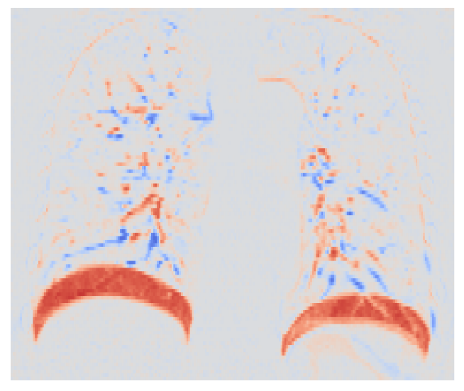

A visual inspection of the deformation fields, as shown in fig. 8 for case 5, revealed that our proposed method produced a more physiologically plausible sliding motion between the thoracic cavity and the lung, particularly in the yellow region of interest (highlighted by the yellow box in fig. 8). In contrast, as depicted in figs. 8 and 8, the vertebra is torn down in an unnatural manner along with the lung. The yellow arrows in the deformation field magnitude images in figs. 8, 8, and 8 indicated that our proposed method generated more discontinuous deformation fields. The difference image before and after registration using our proposed method, shown in fig. 9, demonstrated that our method can achieve an accurate registration result.
6 Conclusion
In this paper, we proposed a novel registration method that combines both zeroth- and first-order momenta based on a multiplicative Wendland kernel within the LDDMM framework. Our method was supported by a mathematical analysis of the derived flow, providing a deeper understanding of the method. The experimental results on synthetic 2D images and a clinical CT dataset showed that our method can effectively preserve discontinuous motions at sliding interfaces. These results demonstrate the potential of our proposed method for improved registration accuracy in medical imaging applications.
References
- [1] M. F. Beg, M. I. Miller, A. Trouvé, and L. Younes, Computing Large Deformation Metric Mappings via Geodesic Flows of Diffeomorphisms, International Journal of Computer Vision, 61 (2005), pp. 139–157, https://doi.org/10.1023/B:VISI.0000043755.93987.aa, http://link.springer.com/10.1023/B:VISI.0000043755.93987.aa (accessed 2022-06-21).
- [2] F. Bizzarri, A. Colombo, F. Dercole, and G. S. Gajani, Necessary and Sufficient Conditions for the Noninvertibility of Fundamental Solution Matrices of a Discontinuous System, SIAM Journal on Applied Dynamical Systems, 15 (2016), pp. 84–105, https://doi.org/10.1137/140959031, http://epubs.siam.org/doi/10.1137/140959031 (accessed 2023-01-09).
- [3] F. Bookstein, Principal warps: thin-plate splines and the decomposition of deformations, IEEE Transactions on Pattern Analysis and Machine Intelligence, 11 (1989), pp. 567–585, https://doi.org/10.1109/34.24792, http://ieeexplore.ieee.org/document/24792/ (accessed 2023-01-13).
- [4] L. Dieci and L. Lopez, Fundamental matrix solutions of piecewise smooth differential systems, Mathematics and Computers in Simulation, 81 (2011), pp. 932–953, https://doi.org/10.1016/j.matcom.2010.10.012, https://linkinghub.elsevier.com/retrieve/pii/S0378475410003186 (accessed 2022-11-11).
- [5] B. Fischer and J. Modersitzki, Curvature Based Image Registration, Journal of Mathematical Imaging and Vision, 18 (2003), pp. 81–85, https://doi.org/10.1023/A:1021897212261, http://link.springer.com/10.1023/A:1021897212261 (accessed 2023-01-16).
- [6] C. Frohn-Schauf, S. Henn, and K. Witsch, Multigrid based total variation image registration, Computing and Visualization in Science, 11 (2008), pp. 101–113, https://doi.org/10.1007/s00791-007-0060-2, https://link.springer.com/10.1007/s00791-007-0060-2 (accessed 2023-01-16).
- [7] Y. Fu, S. Liu, H. H. Li, H. Li, and D. Yang, An adaptive motion regularization technique to support sliding motion in deformable image registration, Medical Physics, 45 (2018), pp. 735–747, https://doi.org/10.1002/mp.12734, https://onlinelibrary.wiley.com/doi/10.1002/mp.12734 (accessed 2022-12-15).
- [8] L. Gong, L. Duan, Y. Dai, Q. He, S. Zuo, T. Fu, X. Yang, and J. Zheng, Locally Adaptive Total p-Variation Regularization for Non-Rigid Image Registration With Sliding Motion, IEEE Transactions on Biomedical Engineering, 67 (2020), pp. 2560–2571, https://doi.org/10.1109/TBME.2020.2964695, https://ieeexplore.ieee.org/document/8951270/ (accessed 2023-01-18).
- [9] D. L. G. Hill, P. G. Batchelor, M. Holden, and D. J. Hawkes, Medical image registration, Physics in Medicine and Biology, 46 (2001), pp. R1–R45, https://doi.org/10.1088/0031-9155/46/3/201, https://iopscience.iop.org/article/10.1088/0031-9155/46/3/201 (accessed 2023-01-19).
- [10] R. Hua, J. M. Pozo, Z. A. Taylor, and A. F. Frangi, Multiresolution eXtended Free-Form Deformations (XFFD) for non-rigid registration with discontinuous transforms, Medical Image Analysis, 36 (2017), pp. 113–122, https://doi.org/10.1016/j.media.2016.10.008, https://linkinghub.elsevier.com/retrieve/pii/S1361841516301888 (accessed 2023-01-13).
- [11] H. O. Jacobs and S. Sommer, Higher-order spatial accuracy in diffeomorphic image registration, Geometry, Imaging and Computing, 1 (2014), pp. 447–484, https://doi.org/10.4310/GIC.2014.v1.n4.a3, http://www.intlpress.com/site/pub/pages/journals/items/gic/content/vols/0001/0004/a003/ (accessed 2022-06-02).
- [12] C. Jud, N. Mori, and P. C. Cattin, Sparse Kernel Machines for Discontinuous Registration and Nonstationary Regularization, in 2016 IEEE Conference on Computer Vision and Pattern Recognition Workshops (CVPRW), Las Vegas, NV, USA, June 2016, IEEE, pp. 449–456, https://doi.org/10.1109/CVPRW.2016.63, http://ieeexplore.ieee.org/document/7789553/ (accessed 2022-10-21).
- [13] R. I. Leine and H. Nijmeijer, Dynamics and Bifurcations of Non-Smooth Mechanical Systems, vol. 18 of Lecture Notes in Applied and Computational Mechanics, Springer Berlin Heidelberg, Berlin, Heidelberg, 2004, https://doi.org/10.1007/978-3-540-44398-8, http://link.springer.com/10.1007/978-3-540-44398-8 (accessed 2022-11-15).
- [14] F. Maes, A. Collignon, D. Vandermeulen, G. Marchal, and P. Suetens, Multimodality image registration by maximization of mutual information, IEEE Transactions on Medical Imaging, 16 (1997), pp. 187–198, https://doi.org/10.1109/42.563664, http://ieeexplore.ieee.org/document/563664/ (accessed 2023-02-01).
- [15] J. Modersitzki, Numerical Methods for Image Registration, Oxford University PressOxford, 1 ed., Dec. 2003, https://doi.org/10.1093/acprof:oso/9780198528418.001.0001, https://academic.oup.com/book/1500 (accessed 2023-01-16).
- [16] J. Modersitzki, FAIR: flexible algorithms for image registration, Society for Industrial and Applied Mathematics (SIAM, 3600 Market Street, Floor 6, Philadelphia, PA 19104), Philadelphia, Pa., 2009. OCLC: 694086088.
- [17] F. P. Oliveira and J. M. R. Tavares, Medical image registration: a review, Computer Methods in Biomechanics and Biomedical Engineering, 17 (2014), pp. 73–93, https://doi.org/10.1080/10255842.2012.670855, http://www.tandfonline.com/doi/abs/10.1080/10255842.2012.670855 (accessed 2023-02-01).
- [18] A. Pai, S. Sommer, L. Sorensen, S. Darkner, J. Sporring, and M. Nielsen, Kernel Bundle Diffeomorphic Image Registration Using Stationary Velocity Fields and Wendland Basis Functions, IEEE Transactions on Medical Imaging, 35 (2016), pp. 1369–1380, https://doi.org/10.1109/TMI.2015.2511062, https://ieeexplore.ieee.org/document/7364268/ (accessed 2022-10-17).
- [19] B. W. Papież, M. P. Heinrich, J. Fehrenbach, L. Risser, and J. A. Schnabel, An implicit sliding-motion preserving regularisation via bilateral filtering for deformable image registration, Medical Image Analysis, 18 (2014), pp. 1299–1311, https://doi.org/10.1016/j.media.2014.05.005, https://linkinghub.elsevier.com/retrieve/pii/S1361841514000784 (accessed 2023-01-25).
- [20] L. Risser, H. Baluwala, and J. A. Schnabel, Diffeomorphic registration with sliding conditions: Application to the registration of lungs CT images., Fourth International Workshop on Pulmonary Image Analysis, MICCAI, (2011), pp. 79–90.
- [21] L. Risser, F.-X. Vialard, H. Y. Baluwala, and J. A. Schnabel, Piecewise-diffeomorphic image registration: Application to the motion estimation between 3D CT lung images with sliding conditions, Medical Image Analysis, 17 (2013), pp. 182–193, https://doi.org/10.1016/j.media.2012.10.001, https://linkinghub.elsevier.com/retrieve/pii/S1361841512001466 (accessed 2022-08-08).
- [22] A. Roche, G. Malandain, X. Pennec, and N. Ayache, The correlation ratio as a new similarity measure for multimodal image registration, in Medical Image Computing and Computer-Assisted Intervention — MICCAI’98, W. M. Wells, A. Colchester, and S. Delp, eds., vol. 1496, Springer Berlin Heidelberg, Berlin, Heidelberg, 1998, pp. 1115–1124, https://doi.org/10.1007/BFb0056301, http://link.springer.com/10.1007/BFb0056301 (accessed 2023-02-01). Series Title: Lecture Notes in Computer Science.
- [23] D. Rueckert, L. Sonoda, C. Hayes, D. Hill, M. Leach, and D. Hawkes, Nonrigid registration using free-form deformations: application to breast MR images, IEEE Transactions on Medical Imaging, 18 (1999), pp. 712–721, https://doi.org/10.1109/42.796284, http://ieeexplore.ieee.org/document/796284/ (accessed 2023-01-13).
- [24] A. Schmidt-Richberg, Registration methods for pulmonary image analysis: integration of morphological and physiological knowledge, no. 7 in Aktuelle Forschung Medizintechnik, Springer Vieweg, Wiesbaden, 2014. OCLC: ocn830354559.
- [25] A. Schmidt-Richberg, R. Werner, H. Handels, and J. Ehrhardt, Estimation of slipping organ motion by registration with direction-dependent regularization, Medical Image Analysis, 16 (2012), pp. 150–159, https://doi.org/10.1016/j.media.2011.06.007, https://linkinghub.elsevier.com/retrieve/pii/S1361841511000946 (accessed 2023-01-16).
- [26] J. Shawe-Taylor and N. Cristianini, Kernel methods for pattern analysis, Cambridge University Press, Cambridge, UK ; New York, 2004.
- [27] S. Sommer, M. Nielsen, S. Darkner, and X. Pennec, Higher-Order Momentum Distributions and Locally Affine LDDMM Registration, SIAM Journal on Imaging Sciences, 6 (2013), pp. 341–367, https://doi.org/10.1137/110859002, http://epubs.siam.org/doi/10.1137/110859002 (accessed 2022-09-19).
- [28] S. Sommer, M. Nielsen, F. Lauze, and X. Pennec, A Multi-scale Kernel Bundle for LDDMM: Towards Sparse Deformation Description across Space and Scales, in Information Processing in Medical Imaging, G. Székely and H. K. Hahn, eds., vol. 6801, Springer Berlin Heidelberg, Berlin, Heidelberg, 2011, pp. 624–635, https://doi.org/10.1007/978-3-642-22092-0_51, http://link.springer.com/10.1007/978-3-642-22092-0_51 (accessed 2022-06-02). Series Title: Lecture Notes in Computer Science.
- [29] A. Sotiras, C. Davatzikos, and N. Paragios, Deformable Medical Image Registration: A Survey, IEEE Transactions on Medical Imaging, 32 (2013), pp. 1153–1190, https://doi.org/10.1109/TMI.2013.2265603, http://ieeexplore.ieee.org/document/6522524/ (accessed 2023-02-01).
- [30] V. Vishnevskiy, T. Gass, G. Szekely, C. Tanner, and O. Goksel, Isotropic Total Variation Regularization of Displacements in Parametric Image Registration, IEEE Transactions on Medical Imaging, 36 (2017), pp. 385–395, https://doi.org/10.1109/TMI.2016.2610583, http://ieeexplore.ieee.org/document/7570266/ (accessed 2022-06-27).
- [31] V. Vishnevskiy, T. Gass, G. Székely, and O. Goksel, Total Variation Regularization of Displacements in Parametric Image Registration, in Abdominal Imaging. Computational and Clinical Applications, H. Yoshida, J. J. Näppi, and S. Saini, eds., vol. 8676, Springer International Publishing, Cham, 2014, pp. 211–220, https://doi.org/10.1007/978-3-319-13692-9_20, http://link.springer.com/10.1007/978-3-319-13692-9_20 (accessed 2023-01-18). Series Title: Lecture Notes in Computer Science.
- [32] L. Younes, Shapes and Diffeomorphisms, vol. 171 of Applied Mathematical Sciences, Springer Berlin Heidelberg, Berlin, Heidelberg, 2019, https://doi.org/10.1007/978-3-662-58496-5, http://link.springer.com/10.1007/978-3-662-58496-5 (accessed 2022-06-01).
- [33] D.-X. Zhou, Derivative reproducing properties for kernel methods in learning theory, Journal of Computational and Applied Mathematics, 220 (2008), pp. 456–463, https://doi.org/10.1016/j.cam.2007.08.023, https://linkinghub.elsevier.com/retrieve/pii/S0377042707004657 (accessed 2022-08-10).