Magnetic and Structural Properties of 5d Osmate Double Perovskites Probed by Nuclear Magnetic Resonance
A Dissertation
Presented to
The Academic Faculty
By
Rong Cong
In Partial Fulfillment
of the Requirements for the Degree
Doctor of Philosophy in the
Physics Department
Brown University
May 2022
Abstract of “Magnetic and structural properties of 5d osmate double perovskites probed by nuclear magnetic resonance”, by Rong Cong, Ph.D., Brown University, May 2022.
The combined effect of electronic correlation and strong spin-orbit-coupling(SOC) can give rise to a variety of exotic quantum phases. Double perovskites provide a simple structure to study the spin-orbit-lattice entangled states. In this thesis, focusing on the 5d osmate double perovskite system, we conduct a combination of work including theoretical model simulation, first-principle calculation, and nuclear magnetic resonance experiments to understand the fundamental physical properties of this material system. For 5d Mott insulator Ba2NaOsO6, by conducting spin-spin relaxation measurements and applying quadrupolar noise spectroscopy, we addressed a long-standing missing entropy problem. We found that quadrupolar noise with a Lorentzian distribution persists up to a high temperature above its structural transition, indicating quadrupolar domains which account for the missing entropy in the system. Also by carrying out a classical Monte Carlo simulation using 4 sites per unit cell for a 5d1 double perovskite model with strong SOC, we found that the non-zero quadrupolar moment arises due to additional symmetry breaking that was not captured in earlier mean-field treatment with 2 sites per unit cell, showing consistency with the two non-zero quadrupolar moments proposed in the quadrupolar phase of Ba2MgReO6. Furthermore, we improved the earlier point charge approximation calculation on the electric field gradient of Ba2NaOsO6 and we identified the local orthorhombic structural distortion for Na-O octahedra in Ba2NaOsO6 of around 0.01Å. Our first principle calculation on Ba2NaOsO6 also found the existence of a staggered orbital ordering pattern accompanying its canted ferromagnetic order, which is characterized by the different selective occupation of d orbitals on the two-sublattice Os ions.
Besides Ba2NaOsO6, we have also conducted comprehensive NMR measurements on its isostructural, isovalent compound Ba2LiOsO6. We found that the metamagnetic transition at 5.75T is possibly a spin-flop transition and the ground magnetic state is more likely to be a 3D antiferromagnet. Electron doping effect on 5d1 Ba2NaOsO6 has also been studied on powder compounds Ba2NaxCa1-xOsO6 (0 x 1). We found that all the doped samples remain as magnetic insulators despite the added electrons. Powder spectrum simulation indicates that similar to the Ba2NaOsO6 case, a ”broken local point symmetry” phase with orthorhombic symmetry occurs above magnetic transition for all doped samples. Under the collinear two sublattices canted AFM model, the ground magnetic states evolve from canted FM state to collinear AFM state with the increase of doping electrons. Whether there is multipolar ordering in these samples needs further study using complementary techniques in the future.
©Copyright 2022 by Rong Cong
This dissertation by Rong Cong is accepted in its present form
by the Department of Physics as satisfying the
dissertation requirement for the degree of Doctor of Philosophy.
Date
Professor Vesna Mitrović, Advisor
Recommended to the Graduate Council
Date
Professor Kemp Plumb, Reader
Date
Professor Brad Marston, Reader
Approved by the Graduate Council
Date
Andrew Campbell, Dean of the Graduate School
Curriculum Vitae of Rong Cong
Rong Cong received her Bachelor of Science in physics from University of Science and Technology of China in 2016 and her Master of Science in physics from Brown University in 2018. She enrolled in the PhD program at Brown University in 2016. She joined Professor Vesna Mitrović lab of Condensed Matter NMR in June 2017 and started her research in the 5d osmate double perovskite. Rong Cong’s research focuses on NMR study on quantum materials including transition metal compounds with strong spin-orbit coupling, topological Kondo insulator and unconventional superconductors. During her study at Brown University, she was awarded the Galkin Foundation Fellowship in 2021.
Scientific Publications
- •
NMR study of charge-density wave structure in kagome superconductor RbV3Sb5, J. Frassineti, P. Bonfá, G. Allodi, R. D. Renzi, E. Garcia, R. Cong, V.F. Mitrovic, B. R. Ortiz, S. D. Wilson, and S. Sanna, in preparation.
- •
Electron doped Mott insulator with strong spin-orbit coupling Ba2Na1-xCaxOsO6, E.Garcia,R.Cong P.C.Forino, P.Tran, P.Woodward, V.F.Mitrovic and S.Sanna, in preparation.
- •
Monte Carlo simulation of a strong SOC model for d1 double perovskites, R.Cong, W. Zhang, N. Trivedi, V.F.Mitrovic, in preparation.
- •
Fermi level tuning and double-dome superconductivity in the kagome metals CsV3-Sb5-xSnx, Y.Oey, B.Ortiz, F.Kaboudvand, J. Frassineti, E.Garcia, R.Cong, S.Sanna, V.F.Mitrović, R. Seshadri, S.D. Wilson, 6, L041801 (2022). [doi.org/10.1103/PhysRevMaterials.6.L041801]
- •
First Principles calculations of the EFG tensors of Ba2NaOsO6, a Mott insulator with strong spin orbit coupling, R.Cong, R. Nanguneri, B.Rubenstein, V.F. Mitrovic, 32 (40), 405802 (2020).
[doi.org/10.1088/1361-648X/ab9056] - •
Evidence from first-principles calculations for orbital ordering in Ba2NaOsO6: A Mott insulator with strong spin-orbit coupling, R.Cong, R. Nanguneri, B.Rubenstein, V.F. Mitrovic, 100, 245141 (2019). [doi:10.1103/PhysRevB.100.245141]
- •
Nature of lattice distortions in the cubic double perovskite Ba2NaOsO6, W. Liu, R.Cong, A.P.Reyes, I.R. Fisher, V.F. Mitrovic, 97, 224103 (2018). [doi:10.1103/PhysRevB.97.224103]
- •
Phase diagram of Ba2NaOsO6, a Mott insulator with strong spin orbit interactions, W. Liu, R.Cong, E. Garcia, A.P.Reyes, H.O. Lee, I.R. Fisher, V.F. Mitrovic, 536, 863-866 (2018). [doi:10.1016/j.physb.2017.08.062]
- •
Impact of hydrogen gas on the inverse spin Hall effect in palladium/cobalt bilayer films, S.Watt, R.Cong, C.Lueng, M.Sushruth, P.J.Metaxas, M.Kostylev,
9, 1-4 (2017). [doi:10.1109/LMAG.2017.2777396] - •
Structure and physical properties of the misfit compounds (PbSe)1.16(TiSe2)m (m=1,2), N.Z.Wang, S.F.Yuan, R.Cong, X.F. Lu, F.B.Meng, C.Shang, X.H.Chen, , 112, 67007 (2016). [doi:10.1209/0295-5075/112/67007]
Presentations
- •
Contributed talk (hybrid) “NMR study on the mixed valence insulator SmB6” at the APS March Meeting (online), 2022.[video]
- •
Galkin fellowship presentation (virtual) “Structural and magnetic properties of 5d osmate double perovskites probed by nuclear magnetic resonance” at Brown University, Providence, RI, 2021.[video]
- •
Contributed talk (virtual) “Monte Carlo simulation of a strong SOC model for d1 double perovskites” at the APS March Meeting (online), 2021.[Slide]
- •
Contributed talk “First Principles calculations of the EFG tensors of Ba2NaOsO6, a Mott insulator with strong spin orbit coupling” at the SPICE workshop: Novel Electronic and Magnetic Phases in Correlated Spin-Orbit Coupled Oxides, Johannes Gutenberg University Mainz, Germany, 2019. [video]
- •
Contributed talk “Determining lattice distortion of Ba2NaOsO6” at the APS March Meeting, Boston, MA, 2019.
Acknowledgements
During my Ph.D. study at Brown University, many people have helped me directly and indirectly, and I would certainly not be able to accomplish this thesis without their valuable support. So I would like to give my deepest gratitude to all of them.
First and foremost I would like to thank my supervisor Prof. Vesna Mitrović. Prof. Mitrović has been greatly supportive during my whole Ph.D. studies and I feel very fortunate to have her as my supervisor. She has guided me into the field of scientific research and taught me how to do NMR experiments and learn interesting new physics from the data. She has also provided me with many great opportunities to meetings and conferences, from which I have gained valuable experience in academic communication. Additionally, her great passion for science and her vision for promising research directions have all been very inspiring for me. I am also appreciative of her connecting me with many collaborators, without whom I am not able to accomplish some computational work and gain a deeper understanding of data interpretation. I also feel very fortunate to see her growing and maintaining a large research group, which is impossible without her hard work and determination. In general, I have learned so much from her. It is my great pleasure to work with Prof. Mitrović and I would like to thank her sincerely.
I would also like to thank Dr. Arneil Reyes for helping me with NMR experiments at NHMFL. Dr. Reyes is very knowledgeable and explained so many useful details about NMR experiments through practical illustration. My gratitude also extends to Prof. Samuele Sanna, who has also taught me not only NMR but also NQR and SR experiments. I also enjoyed the many interesting discussions over zoom when collaborating with him on the 5d doped powder project. Besides experimentalists, I am also grateful to have the chance to collaborate with theorists. I would like to thank especially Prof. Brenda Rubenstein for being so responsive and productive that my first-principle calculation projects went smoothly. She has also provided great editions of my paper writings. And I would like to thank my committee members, Prof. Kemp Plumb, for providing high-quality single crystals and valuable suggestions in collaborating on the study of the GaTa4Se8 compound, and Prof. Brad Marston for giving guidance on the Monte Carlo simulation project.
Apart from professors, I would also like to give my sincere gratitude to my colleague Erick Garcia, who has been particularly reliable and helpful in constructing and developing essential instruments for experiments. I would also like to thank him as a great companion during my whole Ph.D. process for discussing our experiments, traveling to NHMFL and PSI for onsite measurements, and offering help whenever he can. For the interpretation of Ba2NaOsO6 results, I need to thank Dr. Stephen Carr for his insight and great theoretical simulation. Without him, understanding our experimental results would be impossible. For the Monte Carlo project, I would like to thank Prof. Nandini Trivedi and Dr. Wenjuan Zhang for the meeting, discussing, and sharing with me their mean-field calculation approach. For DFT calculations, I want to thank Dr. Ravindra Nanguneri for teaching me to use the software and helping me in completing papers. For NMR experiments related to 5d osmate compounds, I would like to thank Dr. Elizabeth Green and Sanath Kumar Ramakrishna for assisting our measurements at Maglab, and also Prof. Giuseppe Allodi for providing supplementary measurements and powder simulation. Among peer graduate students, I want to thank especially Yiou Zhang for discussing physics with me related to a lot of the projects I have been involved in.
Furthermore, I also need to thank all the graduate students and visiting students I have been working with within the lab, including Calvin Bales, Dr. Wencong Liu, Paola C. Forino, Anna Tassetti, and Jonathan Frassineti, Donovan Davino, Ilija Nikolov, Silverio Johnson, and Zhenxiang Gao. It was a great experience working with you all. Many people outside my lab have also been greatly helpful during my Ph.D. study and I want to thank Yiming Xing, Tsung-Han Yang, Dr. Zekun Zhuang, Dr. Xiaoxue Liu, Dr. Jiang-Xiazi Lin, Dario F. Mosca, Dr. Xue Zhang, Dr. Kang Wang, Dr. Kaiya Wei, Dr. Jiaqiang Yan, Prof. Gang Xiao and Michael Packer.
My greatest gratitude is also to my parents, who have been always encouraging and confident in me all these years while I am pursuing my Ph.D. degree.
CHAPTER 1Introduction
The combined influence of electron correlation and spin-orbit coupling in the heavy transition metal compounds with 4d and 5d elements have received particular research interest recently due to the emergent quantum phases that are predicted to arise in these systems, such as multipolar charge order, spin liquid, Weyl semimetal, topological insulator, and semimetal, and axion insulator, etc [1]. As shown in Fig.1.1, when the on-site Coulomb repulsion U and spin-orbit coupling strength are both relatively small compared to the hopping integral t, we get traditional metal or band insulators. If we increase U, we will enter into the Mott insulator region, where traditional correlated materials have been mainly studied on the 3d transition metal compounds. On the other hand, increasing can induce band gap closure and inversion, resulting in topological insulator or semimetal, which are mainly studied in solids with heavy s- and p- electron elements. Then in the large /t and weak to intermediate correlated region, materials with non-trivial topology, such as axion insulator, Weyl semimetal, and topological Mott insulator, appear, which are mainly studied in the pyrochlore iridates system. Further increasing U will lead to the strongly correlated region where potential spin liquid materials are explored in the 4d/5d honeycomb iridates and quadrupolar or multipolar ordering materials are mainly studied in the 4d/5d double perovskites system. The large atomic number Z of 4d/5d materials enables large spin-orbit-coupling () and the large ionic distance of double perovskites gives a small hopping integral t and large on-site Coulomb repulsion U (due to smaller carrier density thus a larger screening distance), making the system more correlated. The Mott-Hubbard model as shown in Equ.1.1 is the most widely used theoretical model in describing the above materials systems, where ciα is the annihilation operator for an electron in orbital at site i and niα=c is the corresponding occupation number[1].
| (1.1) |

Strongly correlated materials with quadrupolar and multipolar ordering have been mainly studied earlier in the f-electron system[2, 3]. In recent years, many barium based 5d1 and 5d2 materials have been studied[4]. For 5d1 materials, successive symmetry breakings with possible quadrupolar phase have been found in Ba2MgOsO6[5, 6, 7, 8, 9]. High magnetic field induced phase transition has been found in Ba2CaReO6[10]. Three successive phases with possible quadrupole order has been proposed for Ba2CdReO6[11] and a canted ferromagnetic ordering is suggested for Ba2ZnReO6[12]. For 5d2 materials, recent experiments[13] and theoretical calculations[14, 15, 16, 17] have shown that Ba2MOsO6 (M=Zn, Ca, Mg) hold possible ferro-octupolar order or antiferro-qudrupolar order[18], and no orbital or magnetic ordering down to 0.47K has been found for Ba2CdOsO6 from any type of technique[19].
In this thesis, focusing on the central theme of understanding the exotic phases in 5d osmate double perovskite with strong spin-orbit-coupling (SOC), we conduct a combination of work from simulation of theoretical models to first-principle calculation and NMR experiments on 5d1 and doped 5d1 compounds. Our results allow us to address many interesting questions in this field, such as the existence of both the ferro- and antiferro- quadrupolar moments in the proposed quadrupolar phase of Ba2MgReO6[6], the nature of non-zero electric field gradient in the broken-local-point symmetry phase of Ba2NaOsO6 (section 5.2), the existence of orbital / quadrupolar ordering in the presence of canted ferromagnetic order of Ba2NaOsO6 (section 5.3), the long-standing mystery of missing entropy in Ba2NaOsO6 (section 6.1), the possible spin-flop transition in Ba2LiOsO6 (section 6.2), and the structural and magnetic phases in the doped 5d1 compounds Ba2NaxCa1-xOsO6 (0 x 1) (section 6.3).
The thesis is organized as follows. The theoretical background about the 5d transition metal compounds is presented in Chapter 2. We introduce the concepts that are essential to understanding the 5d osmate double perovskite system, such as crystal field splitting, Jahn-Teller effect, orbital and quadrupolar ordering, etc. We also present a summary of the earlier study on the 5d1 double perovskite Ba2NaOsO6 and Ba2LiOsO6. The latter part of this chapter is devoted to the theory of the application of the nuclear magnetic resonance (NMR) technique in solid, especially for magnetic insulators. We discuss the electron-nucleus interaction, concentrating mainly on the hyperfine interaction and electric-quadrupolar interaction in solid. We have taken the example of Ba2NaOsO6, which is one of the main materials we study in this thesis, to illustrate the different contributions to the hyperfine interaction and the calculation of the symmetry of hyperfine tensor. We also discuss the NMR shift and spectrum shape under different magnetic orders and the spin-lattice relaxation rate for localized and itinerate electronic systems.
Having set up the theoretical background for the 5d osmate double perovskite system and the NMR theory on solid, we focus on discussing the experimental aspects of the NMR technique, which is the main probe we have been using to investigate the 5d compounds. The NMR technique is considered to be invented by Isidor Isaac Rabi in 1944 [20] and five Nobel prizes (in physics, chemistry, and physiology or medicine) have been given to breakthroughs of NMR related techniques along with its long history of development. Nowadays, NMR remains a useful and sensitive tool and has broad application in almost all areas of modern physical science. It has also shown potential application in quantum information science and technologies based on the manipulation of a single and an ensemble of nuclear spins. In Chapter 3 we introduce the commonly used NMR sequence, such as free induction decay (FID) and spin-echo as well as typical NMR measurements of the spectrum, spin-lattice relaxation rate and spin-spin relaxation rate . Hardware for NMR setups and their related calculation are discussed at the end of this chapter.
In Chapter 4-6, we present the theoretical, computational, and experimental projects relating to 5d osmate double perovskite compounds respectively, forming a coherent and comprehensive study. In Chapter 7, we study a separate compound, the mixed-valence insulator SmB6, expanding the application of the NMR technique to itinerate electron systems beyond magnetic insulators. The main findings for each project are summarized in Chapter 8 in order of significance. Future applications of these findings are also discussed.
CHAPTER 2Theoretical Background
2.1 The 5d osmate double perovskite system
2.1.1Introduction
Splitting of d electron states in a cubic field
The Hamiltonian of a d electron of transition metal ions in an undistorted perovskite structure can be written as[21]
| (2.1) |
where is the ionic Hamiltonian and is the electrostatic potential of the surrounding six oxygen ions. In 5d transition metal compounds, the second crystal field term can actually be comparable to (or larger than) the exchange splitting that giving rise to the Hunds rule. The solution of Equ.2.1 described by the spherical harmonics needs also to satisfy symmetry considerations when the ion is put into the cubic environment, corresponding to the octahedral group. The character table of the octahedral group is shown in Table 2.1. Table 2.2 shows the character table of the representations of octahedral group using s-,p-,d- and f- atomic orbitals as basis. From these two tables, we can see that
| (2.2) |
meaning that the fivefold degeneracy of the d orbital states are splitted to a doublet eg and triplet t2g levels (g denotes even function in German). Thus the wave functions for the d states can be written as
| (2.3) | ||||
| (2.4) |
for the twofold degenerate eg states and
| (2.5) | ||||
| (2.6) | ||||
| (2.7) |
for the threefold t2g states.
basis E 8C3 3C2 6C2’ 6C4 A1 {x2+y2+z2} 1 1 1 1 1 A2 {xyz} 1 1 1 -1 -1 E {x2-y2,3z2-r2} 2 -1 2 0 0 T1 {x,y,z} 3 0 -1 -1 1 T2 {xy,yz,zx} 3 0 -1 1 -1 , reprint from Ref [21]
l E 8C3 3C2 6C2’ 6C4 0 1 1 1 1 1 1 3 0 -1 -1 1 2 5 -1 1 1 -1 3 7 1 -1 -1 -1
In this case, when the crystal field splitting is larger than the spin-orbit coupling, which is valid for the 5d electron system, complete or partial orbital quenching might happen. The complete orbital quenching happens when electrons are occupying only the eg states since both the and the states have averaged , having no contribution to the orbital magnetic moment. Partial orbital quenching happens when the t2g states are partially filled since the and states can be rearranged to become the eigenstates of ( and ), which contributes non-zero orbital angular momentum in the presence of external field while has . In fact, the partially quenched angular momentum in -states can be considered as a ”pseudo angular momentum” with [21], with effective angular momentum eigenvalue of . The origin of the orbital quenching is that the presence of a crystal field lowers the symmetry of the system and induces further splitting of the energy levels. And if the split energy levels are no longer the eigenstates of , no further Zeeman splitting will happen under an external magnetic field, causing quenching of orbital angular momentum.
Jahn-Teller effect and orbital ordering
Apart from quenching of orbital angular momentum, another phenomenon that is common in the d electron system is the Jahn-Teller effect. The Jahn-Teller theorem states that if the symmetry of the crystal field is so high that the ground state of an ion is predicted to be orbitally degenerate then it will be energetically preferable for the crystal to distort in such a way that the orbital degeneracy is lifted[22]. The appearance of the distortion is the Jahn-Teller effect[23]. In d electron systems with orbital degeneracy, the cooperative Jahn-Teller effect[24] among a large amount of isolated Jahn-Teller centers, which induce a structural transition is also accompanied by the occupation of particular orbitals at each site, called orbital ordering. The relation between the Jahn-Teller effect and orbital ordering is a ”chicken-and-egg problem”[24], which means that they always occur together.
Fig.2.1 shows the d energy level splitting for the case when the Jahn-Teller energy is larger than spin orbit coupling (a) and vice versa (b). In 5d system, the crystal field energy 2eV, Columb repulsion U=1.52eV, Hunds coupling 0.5eV, spin orbit coupling 0.5eV and the Jahn-Teller energy E=0.20.3 eV. So the ground state for the 5d1 system is a j= quartet. Also because of the large extent of the 4d and 5d electrons, the electric quadrupole moment can not be ignored[25]. The quadrupole moment measures what is loosely call the orbital character of the states. The quadrupole moment tensor are defined as[21]
| (2.8) |
For the 3d electronic states, the orbital state is well defined. However, in the case of strong SOC, the quadrupole moment has both the spin and charge contributions. And the quadrupolar ordering refers to the non-vanishing quadrupole moments. Orbital ordering is usually replaced by quadrupolar ordering since the orbital states under strong SOC might be not well defined.

Osmate 5d1 double perovskite
Magnetic Mott insulators with strong spin-orbit coupling [26, 27, 28, 29, 30] has long been a prime focus of strongly correlated materials research because of the complex interplay among their spin, orbital, and charge degrees of freedom. Earlier studies on the 3d system have revealed the dominant importance of electronic correlation due to the large Coulomb interaction while the spin-orbit coupling (SOC) is of minor consideration and is treated perturbatively[1, 31, 25]. It is usually in the 4f system such as lanthanides that the strong SOC becomes competitive with the exchange interaction and even the crystal field[25]. While 3 systems have been studied intensively[32] much less is known about 4 and 5 systems, in which the more delocalized electrons, weaker correlations, and larger spin-orbit coupling (SOC) effects compete to give rise to rich magnetic and electronic phases, including multipolar magnetic ordering, SOC assisted Mott insulators, and topological insulators [25, 33, 31, 1, 34].
The competition between electron correlation and spin orbit coupling (SOC) present in materials containing 4 and 5 transition metals is an especially fruitful tension predicted to lead to the emergence of a plethora of exotic quantum phases, including quantum spin liquids, Weyl semimetals, Axion insulators, and phases with exotic magnetic orders [26, 25, 35, 36, 33, 1, 37, 27, 28, 29, 30, 1]. There has been an active quest to develop microscopic theoretical models to describe such systems with comparably strong correlations and SOC to enable the prediction of their emergent quantum properties [26, 25, 35, 36, 33]. For example, Chen et al. [25] have constructed a projected strong SOC model which avoids the direct treatment of the spin-orbit coupling term by projecting the spin and orbital operators to the total magnetic ground state j=3/2. Ishizuka et al.[36], on the other hand, has used an effective S=1/2 description without consideration of the orbital operator. Romhanyi et al[37]. introduced a spin-orbital model with explicit consideration of the SOC term and focusing on the discussion of the ground state only. In strong Mott insulators, mean-field theories predict strong SOC to partially lift the degeneracy of total angular momentum eigenstates by entangling orbital and spin degrees of freedom to produce highly nontrivial anisotropic exchange interactions [25, 35, 37, 33]. These unusual interactions are anticipated to promote quantum fluctuations that generate such novel quantum phases as an unconventional antiferromagnet with dominant magnetic octuple and quadrupole moments and a noncollinear ferromagnet whose magnetization points along the [110] axis and possesses a two-sublattice structure.
Because their SOC and electron correlations are of comparable magnitude[1], 5 double perovskites with chemical formula A2BB’O6, where B’ are magnetic ions and B are non-magnetic ions have received particular attention due to its frustrated FCC lattice[25, 36, 33], and are ideal materials for testing these predictions. In 5 transition metal oxides with strong spin-orbit coupling, the lower energy t2g triplet can be regarded as a pseudospin operator = -1, which gives rise to the ground state quartet together with [38, 26]. Experiments on Os compounds such as Ba2MOsO6 where M is Na or Li have shown that while the former orders ferromagnetically with an easy axis [110], the latter orders antiferromagnetically, indicating the subtle difference in the exchange interactions in the two systems[39, 40]. We will give a more detailed discussion of the physical properties of these two compounds in the following two subsections.
2.1.2Ba2NaOsO6

Ba2NaOsO6(BNOO) is an fcc double perovskite with unpaired 5d1 Os magnetic ion forming Os-O and Na-O octahedral alternatively as shown in Fig.2.3(b). It is characterized as a Mott insulator from infrared reflectivity (Fig.2.2(a)) with U3.3eV. Magnetization measurements show a ferromagnetic transition at about 8K but with a negative curie Weiss temperature and an effective magnetic moment of 0.6, which is much smaller than the pure spin case of 1.7 (2, s=) as shown in Fig. 2.2(b) and (c). The magnetic easy axis is along [110] which can not be explained by standard Landau theory with cubic anisotropy (Fig.2.2(c)). Also, while the ground state is a j=3/2 quartet, the magnetic entropy is Rln2 (Fig.2.2(d)). The missing entropy had been a long-standing mystery. In Chapter 6 section 6.1, we used the spin-spin relaxation curve with quadrupolar spectroscopy to address the issue and provide details of the development of the BLPS phase. Recent NMR experiments on Ba2NaOsO6 revealed a canted ferromagnetic ground state and an intermediate temperature ”breaking local point symmetry” (BLPS) state [41, 42, 43, 44, 45] (Fig. 2.3(a),(c)), which is first compared to the time-reversal invariant magnetic state from the mean-field calculation of Chen’s model. However, in Chen’s model, the existence of the four-spin and six-spin interactions in terms of the effective spin moment may increase quantum effects from experience[25]. To deal with the issue, more quantitative numerical methods should be applied, such as direct diagonalization, efficient Monte Carlo, etc. Chapter 4 presents the result of a classical Monte Carlo simulation as a numerical calculation on this model to explore if the experimental feature could be reproduced by applying the straightforward classical approximation and how fluctuations are essential to capture the correct physics.

.
Besides, the BLPS phase precedes the formation of long-range magnetic order, which at sufficiently low temperatures, coexists with the two-sublattice cFM order, with a net magnetic moment of per osmium atom along the [110] direction. Several questions that remain are whether is the actual displacement of oxygen ions or the redistribution of electronic charge that gives rise to the BLPS phase and if the cFM order at low temperatures implies the existence of complex orbital/quadrupolar order. Chapter 5 has addressed both questions using first-principle calculations. Similar successive symmetry breaking has also been recently found in another 5d1 compound Ba2MgReO6 [5, 6].

2.1.3Ba2LiOsO6
Ba2LiOsO6 (BLOO) is an isostructural and isovalent compound of BNOO. Susceptibility experiment [40] carried out on this compound has shown an AFM transition at 8K with an effective magnetic moment of (Fig.2.4(a)), which is much smaller than the spin only value, indicating the presence of strong SOC [37]. Muon spin relaxation measurements also reveal a spin-flip transition in the applied magnetic field in the vicinity of 5.5 T at 2 K [46] (Fig.2.4(c)), and no other magnetic transition up to 45T (Fig.2.4(b)). It has revealed that the internal field is a static but spatially-disordered spontaneous field (Fig.2.4 (d)).
2.2 Application of NMR in magnetic materials
2.2.1Electron-nucleus interactions
Hyperfine interaction
The electron-nucleus interaction mainly consists of two terms, the hyperfine interaction and the electric quadrupolar interaction . The Hamiltonian of hyperfine interaction can be written as
| (2.9) |
where the first term is the orbital angular momentum of an electron with the nucleus’s magnetic moment . The second and third terms comprise the dipolar part of the hyperfine interaction , which is the dipolar tensor. The third term is the Fermi contact hyperfine term and is only non-zero for the case of s electron, which has a non-vanishing wave function probability at the atom’s original point. This can be seen from the in the expression. The Fermi contact term is usually the larger and dominant term in the hyperfine interaction since the dipolar term is proportional to and decays quickly when the measured nuclei site is sitting away from the electrons. The Fermi contact term can be further divided into two parts , where the first transferred contact term describes the interaction of electrons’ wave function of a specific atom with a nucleus of another atom mediated through intermediate overlapping wave functions, while the second on-site contact term describes the direct overlapping of electron’s s wave function with the nucleus cite of the same atom. The and correspond to the transferred and on-site contact hyperfine tensors.

Fig.2.5 illustrates the different contributions of hyperfine interactions mentioned above taking the case of Ba2NaOsO6 as an example. The black dotted lines in a circle represent the s orbit for Na 3s, O 3s, and Os 6s electrons. The black solid lobes represent the O 2p and Os 5d electrons. Dipolar hyperfine coupling between the Os 5d electrons with the Na and Os nuclei are represented respectively by the orange dashed lines. The Fermi contact hyperfine interaction of Na 3s and Os 6s electron with the Na and Os nuclei respectively are represented by the pink dotted line. The Os 5d electron has on-site contact hyperfine interaction through the Os 6s electron with the Os nucleus represented by tensor and the solid green line. It also has the transferred contact hyperfine interaction on the Na nucleus mediated by the overlapping of wave function among the O 2p, O 3s, O 2p, and then Na 3s electrons, represented by tensor and the red solid line. In the NMR experiment when we measure the nuclei to probe the behavior of the 5d electron of Os ion, the main contribution of hyperfine interaction comes from the transferred hyperfine interaction mediated by oxygen’s p orbitals with a minor contribution from the direct dipolar coupling of Os 5d to the Na nuclei.

As we can see from Equ. 2.9, the complexity of the anisotropy of hyperfine interaction is usually encoded in the form of the corresponding hyperfine coupling tensor . The form of can be constrained based on symmetry considerations [47]. Fig.2.6 illustrates the Na-Os octehedra where the hyperfine interaction is represented by the hyperfine tensor between each Os atom, labelled by to , with the Na nucleus. Consider the case when the site symmetry at the Na nucleus is orthorhombic so there are three mirror planes , and . We can write the hyperfine tensor , and with the most general form first as
| (2.10) | |||||
| (2.11) | |||||
The mirror reflection matrix about x=0, y=0 and z=0 three planes can be written as
| (2.12) |
Then we can apply the mirror reflection transformation first about the x=0 plane and we will have , , . Here becomes after mirror reflection while and remain the same. Combining the mirror reflection along y=0 and z=0, we have and . This yield the form of and to be
| (2.13) |
Similarly, we can obtain the form for the other tensors to be
| (2.14) |
So the local magnetic field at the Na nucleus site can be calculated to be
| (2.15) | ||||
| (2.16) |
To simplify the description of hyperfine interaction on the Na nucleus site, sometimes we can take the hyperfine tensor at Na site to be an averaged value of to . Also, we see that in this case when we only consider the orthorhombic site symmetry, all the hyperfine tensors should be in diagonal form. However, the deduced hyperfine tensor at Na sites has an off-diagonal term and a different symmetry [41]. This implies the effect of spin-orbit coupling that has produced anisotropy which is not be able to take into account by the symmetry considerations mentioned above.
Electric quadrupolar interaction
The electric quadrupolar interaction comes from the electrostatic interactions , where is the charge density of nuclei and is the electrostatic potential created by the electrons surrounding the nucleus, which can be written as
| (2.17) |
If the electronic charge distribution of nuclei is spherical symmetric or is a spheroidicity with axial symmetry, the electric dipole moment is both zero. However, for the latter case, the electric quadrupole moment is non-zero. The electric quadrupole moment can be written as
| (2.18) |
and the Hamiltonian for electric quadrupolar interaction can be written as
| (2.19) |
where represents the third term in Equ.2.17 and is the electric field gradient (EFG) tensor, and is usually written as the largest absolute eigenvalue of the EFG parameters as . The electric quadrupolar interaction is only non-zero for . This is because the shift of evergy level due to electric qudarupolar interaction in the NMR can be written as to the first order perturbation. And the electric quadrupolar moment as shown in Equ. 2.18 can be regarded as a rank-2 tensor . So and based on the Wigner-Eckart theorem and the corresponding Clebsch-Gordan coefficients [48]. Similarly analysis can be applied to the electric octupolar moments, meaning that the electric octupolar moment is non-zero when nuclei spin and so on.
The EFG tensor , which is more commonly written as , is a symmetric () and traceless () tensor. Three eigenvalues are . The asymmetry factor is defined as and is naturally within 0 and 1 based relationship among the three eigenvalues. The eigenvectors have three principal axes. So after diagonolization as shown as
| (2.20) |
there are five irreducible elements that includes all the information of the electronic environment around the nuclei. usually refers to the axis in the principle coordinate system of EFG.
By calculating the first order perturbation energy level beyond the Zeeman interaction, we can get the expression for quadrupolar splitting as
| (2.21) |
and the and here represent the relative angle of the external magnetic field in the EFG coordinate system, and . Fig.2.7 shows the example of the case for and , where the quadrupolar interaction split the original Zeeman energy levels and gives a triplet with different quadrupolar splitting value when (Fig.2.7(a), (c)) and (Fig.2.7(b), (d)). We need to note that the satellite peaks cross with the central peak when changes from 0 to . The angle when all the three peaks overlap with each other can be determined from Equ.2.21 to be about degree. So the NMR EFG parameters can be determined by measuring the rotation pattern of the spectrum. Chapter 5 section 5.2 has discussed more details about determining EFG parameters for the Ba2NaOsO6 case from the rotation measurements. For a formal derivation and more complicated cases including the second order electric quadrupolar interaction, one can refer to Ref [49, 50, 51]

2.2.2NMR Shift
In the linear response limit, the NMR shift is usually expressed as
| (2.22) |
where and are the natural frequency and external magnetic field, represents the local magnetic field, is the hyperfine coupling tensor and is the local susceptibility. The Hamiltonian of a nucleus in the external magnetic field can be written as
| (2.23) | ||||
| (2.24) |
where is the interaction between an isolated nucleus magnetic moment with external magnetic field. The diamagnetic term is the interaction between magnetic vector potential of the nucleus moment and external magnetic field. And the interaction between two nuclei’s magnetic vector potential is written as , where and .
The first term gives the reference natural frequency of the nucleus and the third term usually contributes to line broadening due to the nuclei dipole-dipole interaction [53]. The quadrupolar interaction term induces line splitting to the first order perturbation as we discussed earlier. The second term induces the diamagnetic shift and the first term of the orbital contribution from hyperfine interaction induces the orbital shift . Respectively, they give rise to the diamagnetic susceptibility and the Van-Vleck susceptibility , which are both temperature independent, based on Equ.2.22. Together they can be considered as the temperature independent chemical shift part . The remaining spin contribution part in the hyperfine interaction gives rise to the temperature dependent shift and thus . It can be further divided to the dipolar part from the dipolar interaction as discussed earlier and the fermi contact part , where represents the core polariztion as shown in Fig.2.5. Therefore the full expression for the NMR shift and the deduced susceptibility can be written as
| (2.25) | ||||
| (2.26) | ||||
| (2.27) |

For condensed matter NMR, the chemical shift is usually much smaller than the spin shift , so it can be neglected in most cases. Besides as we discussed earlier the main contribution to the is the through either the transferred or on-site hyperfine tensors or . We also need to note that the term Knight shift is originally proposed by Walted D. Knight [55] to describe the shift induced by the interaction of the conduction electrons in metal with the nuclei spin[49]. From our earlier discussion, this shift should belong to since the conduction electrons s wave function has a non-zero value at the nuclei site. However, the term Knight shift in contemporary condensed matter NMR research can be used interchangeably with NMR shift, only to be distinguished with chemical shit, and can be referred to all the contributions to the shift from the spin part of the hyperfine interaction. So for magnetic insulators, such as the ones being studied in this thesis in Chapter 6, it is also common to use Knight shift for describing the NMR results. For magnetic insulators in general, Fig. 2.8 illustrates the NMR spectrum and shift for several common magnetic orders. The frequency shift can be obtained by investigating the local magnetic field at the nuclei site shown as
| (2.28) |
and the frequency shift is
| (2.29) |
This shows that depending on the projection of local magnetic moments along the external field direction, different magnetic orders can be determined from the NMR spectrum. For itinerate electron system, such as metal with s conduction electron, the hyperfine interaction can be written as
| (2.30) |
and the Pauli susceptibility is
| (2.31) |
So the Knight shift is calculated to be
| (2.32) |
proportional to the density of states . Application of Knight shift in itinerate electron system can be found in Chapter 7.
2.2.3Spin-lattice relaxation rate
While the NMR shift is an extremely useful observable to detect local static magnetic susceptibility of the sample, the dynamic susceptibility is probed by the spin-lattice relaxation rate , where is the spin-lattice relaxation time. In general, spin-lattice relaxation rate probes the fluctuations and low energy excitations of the ”lattice”. These can include such as scattering of conduction electrons on the fermi surface, magnons, phonons, etc. which will induce the stimulated emission between nuclei energy levels. Spin lattice relaxation rate is proportional to the transition probability , which in magnetic insulators with fluctuating local magnetic field from local magnetic moments, can be calculated as [56]
| (2.33) |
where and represents fluctuation fields on plane and can be written as , and is the resonance frequency. After Fourier transformation, the fluctuation field , hyperfine coupling tensor and the local magnetic moment can be written as
| (2.34) | ||||
| (2.35) | ||||
| (2.36) |
So the spin-lattice relaxation rate in the reciprocal space is written as [56]
| (2.37) | ||||
| (2.38) |
showing that is expressed by the spin-spin correlation function of magnetic moment and measures the component of the imaginary part of dynamic susceptibility and corresponds to the dynamical structure factor that is measured by neutron scattering. In magnetic insulators, long-range magnetic order transition is often accompanied by a divergence of due to critical slowing down, when the correlation length blows up. Since the correlation function follows exponential and power law respectively for gapful and gapless excitations respectively, follows the same temperature dependence of for gapful excitations and for gapless excitations. Application of in studying magnetic insulator can be found in Chapter 6 section 6.2. A maximum value of can also be found when the fluctuation frequency of the excitation in the sample matches the Larmor frequency in NMR measurements. This is referred to as the BPP theory proposed by Nicolaas Bloembergen, Edward Mills Purcell, and Robert Pound [57]. The fluctuation is assumed to follow a thermally activated behavior of , where is a measure of time between two successive ”fluctuations” and is the activation energy. The spin-spin correlation can then be expressed as
| (2.39) |
meaning that the chances of not experiencing a ”fluctuation” in time t decrease exponentially. So can thus be written as
| (2.40) |
where reaches a maximum when . This BPP related peak has been observed in all the 5d1 charge doped samples, same as the ones used for NMR measurements in Chapter 6 section 6.3. Details of the analysis on these peaks can be found in Ref [58]. The occurrence of this BPP peak has also been related to the formation of small polarons in these doped samples[59].
For a general fermi system, the transition probability is calculated based on the scattering of conduction electrons around fermi level. So the is expressed as [60]
| (2.41) |
where the square to the density of states at comes from the initial and final states of the scattering process. For fermi liquid, only electrons around the fermi level contribute to the scattering process, so is proportional to as
| (2.42) |
For s electron, the above equation can be calculated to be
| (2.43) |
Combining Equ.2.32 one can obtain the Korringa relation
| (2.44) |
where . The parameter is usually referred to as the Korringa constant or Korringa product. It is a constant for the Fermi liquid system and is equal to 1 for normal metal. It indicates the presence of ferromagnetic correlation at when and antiferromagnetic correlation at when . Similar relations also hold for p and d electrons. Application of Korringa relation in studying itinerates electron systems can be found in Chapter 7. We need to note that NMR is sensitive to low energy excitations, meaning that the fluctuation rate that NMR is sensitive to is between to Hz. As a comparison, other techniques’ detection bandwidth for fluctuation rate is about 10 to Hz for AC susceptibility, to Hz for muon spin resonance, and to Hz for neutron scattering [61]. So high-frequency fluctuation detected by neutron scattering, such as local dynamic structural distortion, might not be able to be observed in NMR when it is beyond NMR’s bandwidth.
CHAPTER 3Experimental Techniques
3.1 Pulsed NMR measurements
3.1.1Free induction decay
The simplest NMR sequence is free induction decay (FID). In the classical picture, in the presence of a static external magnetic field , the nuclear spins will precess with angular velocity along the field direction in the laboratory frame, which is the Larmor precession. In the rotational frame that is rotating at the Larmor frequency , the nuclear spin is static. If we only plot the projection of nuclei spin magnetization along the field direction , we can represent this case in Fig.3.1 (a). In the quantum picture, for the simplest two-level system, the situation represents a favorable occupation on the lower energy state (exaggeratedly displayed in Fig. 3.1 (a)), although the difference between the occupation of the lower and higher energy levels are tiny. For example, for at 1T and 4.2K, the lower energy state has 50.003 of nuclei[62]. At time t=t1, an oscillating magnetic field is applied perpendicular to the static external field , this is achieved by driving current through a coil. The amplitude of voltage after the amplifier applying to the coil is at the order of Vp=102-3V (before the amplifier, the RF gated out voltage is 1V). An estimation of the amplitude of can be found in the subsection 3.2.2. The square pulse from t=t1 to t=t2 in Fig.3.1 (d) represents a 90 degree (/2) pulse that rotate the magnetization to in the classical picture, while saturating the two energy levels in the quantum picture as shown in Fig. 3.1 (b). Typical 90 degree (/2) pulse is about 0.5 to 10 s. After , in the classical picture, starts to dephase on the plane while also starts to relax back along direction. As shown in Fig. 3.1 (c), in the laboratory frame, the orange and blue arrows of represent the different dephasing speeds due to external field inhomogeneity and spin-spin interactions. The changing magnetization on plane is then picked up by the same coil inducing an oscillating voltage in the coil of , where the initial amplitude V. The amplitude then decays with time constant T, which represents the transverse relaxation time, as . The transverse relaxation is accompanied by the longitudinal relaxation, which is characterized by a time constant . In the quantum picture, it is described by the stimulated emission process of the two-level system[53].

3.1.2Spin echo
Although the FID is the simplest pulse sequence, it has the problem that the transverse spin-spin relaxation time is affected by external field inhomogeneity, which can be written as [63]. The first term comes from the uncertainty of Zeeman energy levels, the second term comes from the spin-spin dipolar process, which is also the dominant term for typical solids, and the last term comes from field inhomogeneity. To get rid of the effect of the last term, a spin-echo sequence can be used. As shown in Fig.3.2, after time =t3-t2 ( ) of the FID sequence (Fig. 3.2 (a)), a 180 degree () pulse is applied through the coil from time t=t3 to t=t4. In the classical picture, the application of the pulse continues to rotate the nuclei transverse magnetization by 180 degrees as shown in the solid orange and blue arrows in Fig. 3.2(b). At the time after t=t4, the transverse magnetization continues to dephase on the plane. In the laboratory frame, the direction of dephasing keeps the same before and after the pulse. For example, in Fig. 3.2 (b) and (c), the direction of dephasing for the nuclei spin in orange is along while that is along - for the nuclei spin in blue.

So after time , the second dephasing period after the pulse will bring all the transverse magnetization together along - direction, forming an echo as shown in Fig. 3.2 (d). Since the difference in dephasing due to external magnetic field inhomogeneity is canceled during the two dephasing period before and after the pulse, only intrinsic origins contribute to the echo signal.
3.1.3Frequency sweep and field sweep
There are two ways to obtain the NMR spectrum, by fixing the magnetic field and sweep frequency and fixing the frequency and sweeping the magnetic field, which is related by . Fig. 3.3 shows the difference between these two ways in the presence of Zeeman interaction and quadrupolar interaction. Fig.3.3 (a)-(c) show the case for Zeeman interaction. As one can see in Fig. 3.3 (b) and (c), if different parts of a spectrum are represented by different values, although the field and frequency sweep contain the same information, the spectrum is reversed. Fig.3.3 (d) illustrates the case for nuclei spin I= with quadrupolar interaction. Since the quadrupolar interaction is field independent, the quadrupolar splitting is also field-independent. In the region where the Zeeman interaction is comparable with or smaller than the quadrupolar interaction, , the situation can be complicated. One can see that in some cases there might be only two quadrupolar peaks for , including the case for nuclear quadrupolar resonance (NQR). This is the intrinsic number of peaks a sample might have that does not relate to its relative orientation (EFG parameters including principle axes etc.) with the external field.

3.1.4Measurements of T1 and T2
The values in this thesis were mainly taken by saturation recovery. The saturation recovery sequence of T1 usually consists of two parts. The first part is to saturate all the energy levels, which is represented by pulse 1 in Fig.3.4 (a). It can be a single 90 degree (/2) pulse or a comb of pulses that separated by time (5T2 T1). For the first case, one needs to wait for time TR 5T1 between each scan to make sure that all spins will relax back to their thermal equilibrium state before applying the next /2 pulse. In real experiments, it is common that a single /2 might not be able to saturate all the energy levels. In this case, a comb of pulses usually works much better in ”killing the signal” and the waiting time does not need to be larger than 5T1. The time and the comb pulse length are both very important parameters to tune to ”kill the signal”. The downside is it usually causes temporary heating during the comb pulses are on, which can be the main issue for low-temperature measurements. The second part is to detect the signal after relaxation, which is represented as pulses 2 and 3 in Fig.3.4 (a). This part can be either an FID or a spin/solid echo. For nuclei spin I= or I but vanishing quadrupolar fluctuation, the saturation recovery T1 curve is . The situation is more complicated for other cases and derivation of the spin-lattice relaxation curves can be found in Ref.[64] given different initial conditions for nuclei spins after a /2 pulse or comb pulses. Other T1 measurement sequences include inversion recovery[63], progressive recovery[65], etc.

Fig.3.4(b) shows the simplest T2 measurement sequence, which includes a spin/solid echo. The waiting time between each scan should be larger than 5T1. The second table is to make sure the signal will appear at the same position in time for all the values in the time table. The T2 curve is usually fitted to either an exponential , or a Gaussian decay , where is the time between two pulses. For exponential decay in general, distribution of the relaxation time in the sample can be taken phenomenologically by a stretched exponent 1 as [66]. Other T2 measurement sequences such as CPMG can be found in Ref.[63].
3.2 NMR Equipment
In this subsection, we will describe the NMR equipment used for the NMR experiments conducted in this thesis. All the NMR experiments have been done either at Brown University or at the National High Magnetic field. At Brown University, two superconducting magnets up to 7T and 10T have been used. The 7T magnet is equipped with a variable temperature insert (VTI) (continuous flow cryostat) that can go down to 4.2K. The 10T magnet is equipped with a dilution refrigerator that can go down to 50mK. The NMR spectrometer we used is Magres2000 designed and constructed by Dr. Arneil Reyes at the National High Magnetic Field Laboratory (NHMFL).
3.2.1Data acquisition
Fig.3.5 shows the schematic of the NMR setup for pulsed NMR measurements. The red lines and components represent power transmission and the green lines and components represent power reception. The transmission and reception ”traffic” is separated by the duplexer, which connects to the probe when the pulse is on and switches to the receiver when the pulse is off. Details of the construction of the duplexer can be found in Ref[67]. The pre-amplifier on the reception line has a very low noise figure, which means that the pre-amplifier itself does not introduce noise in the signal chain. The power amplifier on the transmission line has a higher noise figure and is used to amplify the input power. The signal after the pre-amplifier is further amplified in the Magres2000.

The signal coming from the probe is separated into real and imaginary parts by quadrature detection, which allows the detection of both the and components of the magnetization without two orthogonal coils. This is achieved by feeding the receiver reference frequency into two mixers that differ in phase by 90 degrees. The outcoming signals from the two mixers are then orthogonal to each other. An illustration of quadrature detection is shown in Fig.3.6. The time-domain signal is converted to spectrum in the frequency domain as shown in Fig. 3.7. The Fourier transform can be represented by . Here consists of both the real and imaginary parts of the magnetization signal in the time domain and and represents the absorption and dispersion spectrum in the frequency domain.


The transmission bandwidth in the frequency domain is determined by the pulse length. Since the Fourier transform of a square pulse signal is a sinc function, the frequency window is usually taken as the full width of half maximum of the sinc function’s main peak, which is approximate to be , where is the pulse length.
During data acquisition, one might come across the ring-down effect that does not completely die out when the data acquisition starts, which should be excluded from the real signal. The ring-down can come from two origins, ring-down from the circuit and ring-down from other mechanical parts. Ring-down from the circuit can be improved by reducing the quality factor Q of the RLC circuit with the cost of reduced sensitivity in the selective frequency. In a RLC circuit, , and the current in the circuit decays as with the time constant . So reducing Q will reduce the time constant to eliminate the duration of ring-down. The typical Q value is kept between 20-and 30. Ring-down from the mechanical part comes from the fact that under a relatively high magnetic field if there is a large current going through the coil, due to the Lorentz force, the coil might move and induce a ring-down effect. The moving wire causes a moving current which induces a changing magnetic field. This magnetic field will generate its current that in the end be picked up by the coil. So a larger magnetic field makes it easier to have this ring-down effect from mechanical parts. The Lorentz force experienced by the coil is similar to the force that it experiences during a magnet quenching which causes it to move, except that in the latter case the Lorentz force is induced by eddy current while in the former case, it is induced by the driving current. To eliminate the mechanical ring-down effect, one may immerse the coil completely inside epoxy to make it rigid and fix its position to reduce the possibility of it moving. This will also help with preventing the arcing effect.

3.2.2Probe, circuit and coil
Fig. 3.8 shows a probe used for measurement at Brown University which is constructed by Erick Garcia. The RF signal is fed into a coaxial cable with 50 impedance. The single-axis goniometer is made of Polychlorotrifluoroethylene(Kel-f) which has a low coefficient of thermal expansion. There are two configurations for the RLC circuit as shown in Fig.3.8 (c) and (d). The tuning capacitor CT is used to tune the RLC circuit to the desired resonance frequency while the matching capacitor CM is used to match the circuit to 50 impedance for optimal absorption. The NMR coil is usually hand-made using copper or silver wires and should fit the dimension of the sample perfectly. The filling factor represents the ratio of the volume of the sample with the volume that the coil encompasses. The oscillation magnetic field H1 generated by the coil can be from 10-100 Gs. An estimation can be deduced from the 90-degree pulse length. In the classical picture, the tipping angle . Considering a typical 90 degree pulse of and a gyromagnetic ratio of . The corresponding field will be 50 Gs. The coil can be immersed in epoxy to minimize arcing. Arcing can happen between any parts that have a voltage breakdown during pulsing. Severe arcing inducing flashing electric spark can be seen especially in a helium gas environment. Once the position of arcing is located, a solder mask can help for insulating the surface. The signal to noise (S/N) of the NMR experiment depends on many factors. For example, the NMR signal is proportional to the number of scans N and the noise obeys Poisson distribution (), so signal to noise S/N . Also since based on Curie Weiss law, the S/N . And since the larger the external magnetic field (resonance frequency), the larger the population difference (with the Boltzman factor e), and the amplifier’s efficiency is proportional to , S/N is proportional to (or ).
CHAPTER 4Monte Carlo Simulation on the 5d1 Double Pervskite Model with Strong Spin Oribt Coupling
4.1 Introduction
In this chapter, we will study a microscopic model for double perovskites magnetic Mott insulator with strong spin-orbit coupling and multipolar spin interactions[25] by Monte Carlo simulation. The study[70, 71] is inspired by an NMR experiment on a typical magnetic Mott insulator Ba2NaOsO6 which has revealed exotic quantum phases[41]. Our model and approach are different from Ishizuka’s model[36] in the sense that both the spin and orbital operators in the Hamiltonian are projected to the total basis. It also differs from Chen’s treatment[25] since is regarded as a classical vector and 4 sites per unit cell instead of 2 sites are considered in our case. By magnetic annealing, we obtained the low-temperature phase diagram involving both spin and orbital degrees of freedom. The low-temperature ground states consist of a ferromagnetic 4-sublattice (FM 4-sub) with two-sublattice orbital ordering and an antiferromagnetic 4-sublattice (AFM 4-sub) with uniform orbital ordering. The finite temperature states consist of the aforementioned AFM 4-sub and a quadrupolar state. We compared the phase diagram obtained here with two mean-field calculations and we found that the coplanar FM[110] state found in mean-field calculation can not be reproduced under a classical basis because of the constraint of single occupation and strong SOC for the 5d1 system. This reveals that, unlike the AFM 4-sub state, the coplanar FM[110] is a unique quantum state that does not have a classical correspondence. Also, we found that contrary to the mean-field phase diagram, the intermediate temperature quadrupolar state is only supported when the electric-electric quadrupolar interaction V is large, resulting in the phase diagram a large region that has a single transition from a high-temperature paramagnetic state to a low-temperature ferromagnetic state. We attribute this melting of the quadrupolar state to the thermal fluctuation at finite temperature in the Monte Carlo simulation that is not included in the mean-field calculation, which tends to favor more ordered states. Also contrary to the single non-zero quadrupolar moment found in mean-field calculation[25], we found there are two non-zero quadrupolar moments in the quadrupolar state, where the ferroic quadrupolar moment comes from additional symmetry breaking that is not captured in the mean-field treatment with 2 cites per unit cell. This is consistent with the recent experimental results on the local structural distortion on Ba2MgReO6[6] and was not obtained by earlier mean-field calculation[25].
This chapter is organized as follows. First, we will introduce the microscopic model and our classical sampling approach under the constraint of a 5d1 double perovskite with strong SOC. And then to better understand the low temperature and finite temperature phase diagram, we will first discuss the magnetic and orbital states of the model when there is only a single non-zero coupling constant. We will then also show how the system evolves from a ferromagnetic state to the ordered state. After that, we will present the low and finite-temperature phase diagrams, focusing on a comparison with two other mean-field calculation results [25, 33]. And in the end, we will discuss our findings emphasizing the two non-zero quadrupolar moments due to additional symmetry breaking that shows consistency with experiments but was not earlier obtained by the corresponding mean-field calculation.
4.2 Model
The microscopic model we studied in this Chapter is adapted from Ref [25]. It contains four exchange interaction terms calculated from second order perturbation. The Hamiltonian is written as =+++. The first term is the nearest-neighbor antiferromagntic exchange, which is introduced for the electron virtual transfer through oxygen p orbitals and it is written as
| (4.1) |
where
| (4.2) |
Here operators and represents the spin and occupation number on orbital for site respectively. The second term is the nearest-neighbor ferromagnetic exchange due to spin transfer through orthogonal orbitals in the exchange path and it is written as
| (4.3) |
where
| (4.4) |
The third term is the electric quadrupole-quadrupole interaction. It is written as
| (4.5) |
and
| (4.6) |
This term is considered because the 4d and 5d electrons carry electric quadrupole moment. And since these d electrons are extended, their mutual interaction could be large and can not be ignored. The last term is the on-site SOC. Detailed origin and specific form of these interactions can also be found in Ref [25]. The total Hamiltonian needs to be projected to the total effective moment j=3/2 quadruplets. Here we listed the following projection on the plane of the orbitally resolved spin operator and occupation number . This relationship can be checked by using the projection operator and acting the spin operators on the total j = 3/2 basis[25].
| (4.7) |
| (4.8) |
| (4.9) |
| (4.10) |
Then in the projection basis, the Hamiltonian can be written as 1. Although neither nor follow SU(2) algebra, the Hamiltonian has a hidden SU(2) symmetry and an approximate continuous symmetry[25].
The Monte Carlo simulation is based on standard Metropolis algorithm on the magnetic ions of a double peroskite structure, which is a fcc lattice with four distinct sites in a unit cell. The unit vector connecting nearest neighbor sites are :
| (4.11) |
The total effective magnetic moment is treated as a classical vector with length == . The single occupancy condition for the d1 system requires that[25]
| (4.12) |
and
| (4.13) |
The total effective magnetic moment is then restricted in the available solid angle space as shown in the Figure 4.1. The forbidden directions that are indicated by red arrows can be regarded as a ”more quantum” region that is not accessible on a classical basis. Since the coplanar canted FM[110] state has spins pointing in the vicinity of the [100] direction, which resides in the forbidden regions as shown in Fig.4.1, the FM ground state is found to be the FM 4-sub instead of the coplanar canted FM[110] state. This indicates that unlike the AFM 4-sub that are both found using quantum basis by mean-field calculation and classical basis using classical Monte Carlo, the coplanar canted FM[110] is a unique quantum state for 5 system that does not have a classical correspondence.

In the following section, we will first study the magnetic and orbital states when there is only a single non-zero parameter in the model.
4.3 Characterization of the system with single non-zero parameters
4.3.1=1, =0, =0
The pure antiferromagnetic coupling exchange only case has the same magnetic and orbital states as that described for the AFM 4-sub in the main text, so only additional characterization will be mentioned here. To study the anisotropy of the staggered magnetization on plane[36], we calculate where
| (4.14) |
with and = and . The sum over is for all the atoms in the system. As shown in Fig. 4.2 , the temperature dependence of shows a first order like transition at , close to that of the orbital ordering transition. The tipping angle away from the crystalline axis is 45 degree. To show this pattern, we calculate
| (4.15) |
where tan. will approach -1 as the spins points to the diagonal directions on plane. Fig 4.2(d) shows that the transition also happens at around . Fig 4.2(e) shows the temperature evolution of inverse susceptibility, where , and with calculated as
| (4.16) |
The green shows antiferromagnetic transition on plane, while the blue corresponds to the Ising type fluctuation along axis. The inset shows the deviation of and from the paramagnetic linear behavior below . Correlation function is obtained by
| (4.17) |
Fig 4.2(g) shows that below the transition temperature Tc, the system has antiferromagnetic correlation for the transverse components (i.e. on the plane). This is because the transverse correlation function shows oscillating behavior with the increase of the distance from the origin. The non-decaying oscillation behavior also indicates the strong long-range antiferromagnetic correlation and its absolute convergence within the finite system sizes studied. However, as shown in Fig 4.2(f), the longitudinal correlation function decays to 0 when is increased from the origin point. This suggests that there is no magnetic order for the longitudinal component. The component of the spins are fluctuating randomly in the system while they are ordered antiferromagnetically for and components.
4.3.2=0, =1, =0
The pure ferromagnetic coupling exchange only case has the same magnetic and orbital states as that described for the FM 4-sub in the main text, so only additional characterization will be mentioned here.In this case, the temperature dependence of the order parameter (Fig 4.3 (d)) shows a second order like phase transition, where is calculated as
| (4.18) |
and is the component of net magnetization . The temperature dependence of , also calculated from Equ. (4.14) (Fig. 4.3 (e)), shows the second order like phase transition at the temperature , same as that for the orbital ordering and ferromagnetic transition. Fig. 4.3 (f) shows the temperature evolution of inverse susceptibility calculated from Equ. 4.16. The inset shows deviation of Curie-Weiss behavior of the inverse powder susceptibility around the ferromagnetic transition, indicating a small but negative Curie-Weiss temperature. This behavior has recently been seen in both Ba2NaOsO6[39] and Ba2MgReO6[5], where their ferromagnetic behavior coexist with a negative Curie-Weiss temperature. Fig. 4.3(h) shows the transverse long-range antiferromagnetic ordering on the plane, the same as the correlation function discussed for the AFM 4-sub state of the purely J1 case. On the other hand, the longitudinal correlation function as shown in Fig. 4.3(g) reveals the long-range ferromagnetic order, which barely decays within the range of the studied system.
4.3.3=0,=0,=1
The purely quadrupolar only case shares the same magnetic and orbital properties as that described for the intermediate temperature quadrupolar state in the main text, so only additional characterization will be mentioned here. To study its magnetic properties, we calculate the three dipole operators and the five quadrupole operators of this state. As shown in Table 4.1, the components of magnetic multipoles can be decomposed into irreducible representations of the cubic group, which characterizes the symmetry of the ideal double perovskite structure[25]. While all the dipole moments vanished for this state, the quadrupole operators and for the four sublattices A, B, C, and D are non zero as shown by Fig, 4.4(d). The transverse and longitudinal inverse susceptibility deviates oppositely from the linear paramagnetic behavior below , resulting in a perfectly linear powder inverse susceptibility shown in Fig. 4.4 (e). Both longitudinal and transverse correlation functions show that there is no long-range magnetic order below the orbital ordering temperature , as seen in Fig 4.4 (f).
| Moment | Symmetry | Operator |
| Dipole | ||
| Quadrupole | / | |
4.3.4Evolution from ferromagnetic to quadrupolar state
The In this subsection, we show how the system evolves from a magnetically ordered state to a nonmagnetic quadrupolar state by studying the ground state when goes from 0 to infinity ( is set to 0 here). The magnetic ground state along the line evolves with the increase of fluctuation and symmetry from the FM 4-sub to FM 4-sub(b), FM 4-sub(c) (will be described later), and in the end, the non-magnetic state. We characterize each state by three order parameters: the staggered magnetization on plane for two neighboring planes ( and ) as and , and the net magnetization along axis as . The staggered magnetization has the same expression as Equ.4.14 while only takes 1 for plane and only -1 for plane . The net magnetization has the expression of Equ.4.18 while takes only the component. Figure 4.5 shows the temperature dependence of the three order parameters when is equal to 1, 1.5, 3, and 10, which corresponds to the FM 4-sub, FM 4-sub(b), FM 4-sub(c), and the non-magnetic state. We see that for the FM 4-sub state, all the three order parameters are non-zero at the ordered state, then for the FM 4-sub(b) state, the staggered magnetization on one plane vanishes while the other two order parameters remain. For the FM 4-sub(c) state, both staggered magnetization on two planes ( and ) vanish, and for the quadrupolar case, all the three magnetization order parameters vanish. The corresponding spin direction alignments for each state are also attached to the inset. We see that with the increase of , the fluctuation of spins on each layer is increased and the staggered magnetization on the plane vanishes from only a single layer (FM 4-sub(b)) to both layers (FM 4-sub(c). This process is also shown from the correlation functions , and . Fig 4.6 shows the correlation functions for different values. When =1, the ground state is still the FM 4-sub state with transverse antiferromagnetic correlation and longitudinal ferromagnetic correlation. When is increased to 1.5, one of the transverse correlations quickly decays while the other one still holds. This comes from the fluctuation of spin alignments on a particular layer, as shown in the illustration of spin alignments in Figure 4.5 (b), while on the neighboring layer, the spins still form antiparallel pairs. This ground state is labeled as FM 4-sub(b). Then when reaches around 3, both transverse correlation functions start to quickly decay and the spin on both layers fluctuates (as shown in Figure 4.5(c)). However, the system still has the non-zero longitudinal magnetization as shown in the ferromagnetic correlation function. This ground state is labeled as FM 4-sub(c). At the end, when is 10, the system approaches the purely case and the state with vanishing magnetic dipolar moment becomes the ground state. The correlation functions Gxx, Gyy and Gzz decay to zero when is larger than zero, indicating no long-range magnetic order. Additionally, Fig. 4.7 reveals the increasing region for the quadrupolar state, which is characterized by the dipolar and multipolar magnetic moments, as is increasing.
4.4 Low and intermediate temperature states
The ground state phase diagram contains the FM 4-sub and the AFM 4-sub. When V/J1 and J2/J1 are small, the ground state is an AFM 4-sub state with Ising type fluctuation and uniform orbital ordering. The electron occupancy on and are same while that on orbital is minimized (Fig 4.8 (b)), which can be expressed as
| (4.19) | ||||
This was understood as the distinguished axis lifts the degeneracy of triplet, favoring higher occupancy of and orbitals[25]. The zero temperature limit of the electron occupancy are , consistent with that of the mean field results[25]. The total magnetization vanishes with Ising type fluctuation along axis. The spins on the same layer form antiparallel pairs while staggered by 90 degree on neighboring layers as shown in Fig 4.8(b) (), same as the orbital pattern found in Ref. [33]. The characterization of this anisotropy and other quantities have been discussed in the last section.

When V/J1 and J2/J1 are increased, the ground state is a FM 4-sub state with a two sublattice orbital ordering stacking along the direction of magnetization. Suppose symmetry breaking picks up the magnetization along +, then for the A sublattice, the orbital has the highest electron occupancy followed by while it is reversed for the B sublattice. This can be expressed as
| (4.20) | ||||
In both sublattices, orbital has the lowest electron occupancy, which is a direct consequence of Eq.4.10. This orbital pattern with the onset of ferromagnetism is also found in Ref.[33]. The intuitive physical origin they provide is that this orbital pattern reduced the electron overlap on neighboring layers while allowing the electrons to hop from the yellow orbital on the upper layer of Fig 4.8(a) to the less occupied yellow orbital in the layer above or below it (similarly for the red orbitals), which causes the ferromagnetism more energetically favorable[33]. The total magnetization aligns with one of the crystalline axis () and on the plane perpendicular to magnetization, spins on each plane form antiparallel pairs and are staggered by 90 degrees between neighboring layers, as shown in Fig 4.8(a). This is also the case as found for the FM state in Ref[33]. The tipping angle away from the crystalline axis is about 10 to 15 degrees. Details of the characterization of this state have been discussed in the last section.
4.5 Finite temperature phase diagram
The finite-temperature phase diagram is shown in Fig.4.11(b). The phase diagram consists of four regions. In Region I, the ground state is AFM 4-sub lattice. Region II, III, and IV have FM 4-sub lattice as ground state and Region II supports an intermediate temperature quadrupolar state and Region III supports an intermediate temperature AFM 4-sub state while Region IV has a single transition from PM to FM 4-sub state. Fig. 4.9 show the evolution of the orbital order parameter ( are , or ) and net magnetization order parameter for representative cases at each region.

The intermediate temperature magnetic quadrupolar state has vanished net magnetization () with one principal axis (denote by ) distinguished from the other two (denoted by ) as shown in Fig. 4.8(c). The two sublattices orbital ordering has either the highest electron occupancy on or orbitals with the lowest electron occupancy on or , as shown in the lower and upper layer of Fig. 4.8(c). This orbital order can also be expressed by Equ. 4.20 and its temperature evolution can be seen from Fig.4.9(b). For the spin order, the spin moments on the same layer point along with one of the equivalent principal axes with the spins on the neighboring layers points along the other perpendicular axis (Fig. 4.8(c)). And for the spin on each site, the four available directions that the spin can point to are equivalent and there is no pattern or symmetry for the four spins in a single unit cell. These indicate that the fourfold (C4) rotations about the , , and axes are broken as well as the combination of the C4 rotation along the axis and a translation exchanging the A and B sublattices. The latter remains a symmetry for the quadrupolar state in Ref.[chen2010exotic] which considers 2 sites in a unit cell, resulting in the vanishing quadrupolar moment /n. In this Monte Carlo work with 4 sites per unit cell, all the dipole magnetic operators vanish for the quadrupolar state and there are two non-zero quadrupolar moments /n and /n. Definitions of dipolar and multipolar moments can be found in Table 4.1. The magnetic quadrupolar moments can also be expressed by orbital occupation operators and Equ.4.21 shows their relationship[25].
| (4.21) | ||||
For Region II and III that have successive transitions, Fig.4.13 show the transition temperatures at different values of electric quadrupolar interaction . We see that in Region II, the magnetic and quadrupolar transition temperatures and are both linearly proportional to the ferromagnetic exchange coupling but with different slopes. The slope is independent of the value of , as well as the magnetic transition temperature . On the contrary for Region III, the values of the intermediate temperature transition (from PM to AFM) are independent and linearly proportional to with the same slope but the lower temperature transition temperature varies for different . This –dependence of rises because the underlying quadruple orders of the two magnetic structures (FM 4–sub below and AFN 4–sub between and ) differ significantly, as shown in Fig. 4.9 (c). The corresponding energetics carried by become evident in determining the transition temperature , as compared to being irrelevant in determining where the key driver of magnetic transition is the exchange coupling strength .

We can compare the phase diagram of the current Monte Carlo simulation with two mean-field calculations on the same system as shown in Table I. Both Chen’s work and this work used the projected Hamiltonian and are in the strong spin-orbit coupling limit while Chen’s work is done on the j=3/2 multiplets with 2 sites for unit cell and this work is done on the classical vector j basis with the number of sites in the simulation goes from to . Zhang’s work is done in the range of finite spin-orbit coupling and the spin and orbital quantum numbers s and l are considered independently. All three works found FM and AFM ground states and an intermediate temperature quadrupolar state. Chen’s work and the current work also have a region (Region III) that supports the AFM state as an intermediate temperature state, which is not present in Zhang’s work. This is probably because the Hamiltonian in Zhang’s work included an extra AFM term that is not present in the other two works. The main difference in this work is that the coplanar canted FM[110] ground state is found to be an FM 4-sub state. This is because the coplanar canted FM state is prohibited on the classical basis. This is because the strong SOC limit combined with the single occupancy condition for the 5d1 system restricted the available sampling space to a subspace of 4 solid angle. And the directions of for the coplanar canted FM state falls outside of this subspace. Instead, an FM 4-sub state is obtained as the ground state. This means that unlike the AFM 4-sub ground state (which is found to be the AFM 2-sub in Chen’s work since 2 sites per unit cell are used), the coplanar canted FM [110] state is a unique quantum state that does not have a correspondence in classical basis.
Chen (2010) MC simulation Zhang(2021) Hamiltonian H’(,,V,)=H(,,V,) +(,) SOC finite Basis of Hamiltonian j=3/2 multiplets classical vector s=1/2, leff=-1 Method mean field classical Monte Carlo mean field Number of sites/(unit cell) 2 (63,83,103,123) 4 4 Low temperature ground states FM[110] AFM 2-sub FM 4-sub AFM 4-sub Canted FM AFM 4-sub Intermediate temperature states Quadrupolar AFM 2-sub Quadrupolar AFM 4-sub Quadrupolar
The finite-temperature phase diagram is shown in Figure. 4.11(b) on top of the low-temperature phase diagram. Direct comparison of the phase diagram with Chen’s and Zhang’s work are also shown in (a) and (c). The label I, II, and III represent the three corresponding phase diagram region found in the current work and Chen’s work. The solid and dotted lines represent the corresponding finite temperature phase boundaries. As shown in Figure 4.11(b), the region I has a single transition from paramagnetic state to AFM 4-sub state. In region II, the system has an intermediate temperature quadrupolar state and the low-temperature FM 4-sub state. In region III, the system first has a transition from the paramagnetic state to the AFM 4-sub state and then has a transition to the FM 4-sub state at a lower temperature. We see that compared to Chen’s work, the current work has a new region IV where there is only a single transition from paramagnetic state to FM 4-sub state. To further study the details of this difference, we have plotted the temperature evolution of the dipolar and quadrupolar moment operators for three representative points on the phase diagram, each falls into the different regions on the phase diagram respectively. A comparison of these temperature evolutions of moments is shown in Figure. 4.13.

We see that on the first column, which corresponds to the green dot on the region I, the Monte Carlo simulation from the current work (Figure.4.13(b)) has a reduced value on the quadrupolar moments /n (where n is the total number of sublattices) than the mean-field results (Figure. 4.13(a)), indicating the influence of thermal fluctuation considered in the Monte Carlo simulation, since mean-field calculation would favor a more ordered state with a larger value of order parameter. In the second column, the temperature evolution reflects the successive transitions from PM to AFM, and from AFM to FM state in Figure 4.13(d) and (e). The difference in their absolute values of the dipolar and quadrupolar moments comes from the fact that the FM state is found to be the coplanar canted ferromagnetic state while the Monte Carlo obtained the FM 4-sub lattice due to classical restrictions mentioned above. In the third column, we see that in the temperature region where the sublattice-averaged staggered quadrupolar moments /n start to become non-zero in the intermediate temperature region on Figure 4.13(d), the Monte Carlo simulation results obtained vanishing staggered quadrupolar moments while the onset of the magnetic transition happens at around the same temperature as in the mean-field calculation. This intermediate temperature region with vanishing staggered quadrupolar moments in Monte Carlo simulation reveals the melted quadrupolar ordered region when the electric quadrupolar interaction V is not large enough. When V is large, as shown in Figure 4.13 (b), the Monte Carlo simulation also obtains the intermediate temperature quadrupolar phase.
We note that the third row with Figure 4.13 (c),(f), and (i) are plotted with as the x-axis, which can not completely correspond to the x-axis used for the other two works. Nevertheless, one can see that the sublattice-averaged quadrupolar parameter /n is consistent with (a) and (b). The difference between those in (f) compared with (d) and (e) comes from the fact that Ref.[33] does not have a phase diagram region that has successive transitions from PM to AFM to FM as mentioned earlier probably due to the small differences in the AFM Hamiltonian[33]. So Figure 4.13 (f) reflects the transition from PM to quadrupolar to canted FM ordered state. In Figure 4.13 (i), one can see that the quadrupolar state has two non-vanishing quadrupolar moments /n and /n, which is different from what is shown in (g). This is because (i) is carried out in the finite SOC case with 4 sites per unit cell while (g) is in the infinite SOC case with 2 sites per unit cell. Taking the infinite SOC limit in (i) will lead to two non-vanishing quadrupolar moments (see Ref [33] Appendix F). However, in the Monte Carlo simulation with an infinite SOC limit and 4 sites per unit cell, the quadrupolar order is characterized by two non-vanishing quadrupolar moments (see Figure 4.4 and Figure 4.7). The non-zero ferroic quadrupolar moment /n comes from the additional symmetry breaking that is not captured in the earlier mean-field treatment with 2 sites per unit cell. Fig.4.12 shows the spatial distribution of effective moment in the quadrupolar state for the purely quadrupolar V=1 case. As shown in the subplot (a), the vectors , and , point to four different directions respectively. Moreover, to see if there is any certain pattern in a single unit cell, we plot the spatial distribution of vector for all the unit cells when it is pointing to the same quadrant as shown in Fig.4.12 (b). We then plot the spatial distribution of the other three j vectors in those unit cells as (c), (d), and (e). We see that when lies in a certain quadrant, the other three vectors , and can lie in any of the four quadrants and there is not a certain pattern followed by a single unit cell. And the C4 rotation about axis with a translation of A and B sublattice, which remains as a symmetry for the quadrupolar state found in Ref.[25] using 2 sites per unit cell, is broken here, giving rise to the non-zero quadrupolar moment /n. The two non-zero quadrupolar order parameters have also been found experimentally in Ba2MgReO6[6].

4.6 Summary and Discussion

In summary in this chapter, we carried out a classical Monte Carlo simulation of a projected strong SOC model for a 5 double perovskite system. We found that in this system the coplanar canted FM[110] state is a unique quantum state that does not have a correspondence on a classical basis. And by comparison with the mean-field phase diagram, we found that thermal fluctuation, which is included in Monte Carlo simulation but not in the finite temperature mean-field, plays an important role in determining the size of the region with the intermediate temperature quadrupolar state. The intermediate temperature quadrupolar region is reduced to the large V parameter region while the other quadrupolar region in the mean-field approximation melt, probably due to thermal fluctuation. The quadrupolar transition temperature is linearly proportional to the / and while the lower temperature magnetic transition temperature is independent of .
The result can find a direct application on real materials such as the 5 double perovskite compounds Ba2MOsO6 with M=Na, Li, and Ba2MgReO6[5]. The broken local point symmetry phase found from the NMR experiment for Ba2NaOs and the intermediate temperature phase found in the specific heat measurement of Ba2MgReO6 can both be related to the intermediate temperature state here. Specifically, as we mentioned earlier, in the region II in Fig.4.11 where the system supports a quadrupolar state,
there are always two non zero quadrupolar moments /n and /n with /n larger than /n. We note that this result is not due to the sampling restriction as discussed in section 4.2, since the restriction is only applied to the magnetic moment and not the orbital moments which are directly related to the quadrupolar moments as shown in Table 4.1. This means that can take all the possible values same as that in the mean-field calculation.
Experimentally, this has also been observed in Ba2MgReO6 with being the dominant quadrupolar moment, consistent with our calculation. This reflects that considering 4 sites per unit cell is essential to obtain the quadrupolar state that can be matched with experimental results. For the AFM case, experimentally Ba2LiOsO6 is characterized as an antiferromagnet, although the details of its magnetic order have not been revealed. It also displays a metamagnetic transition at around 5.5T. It would be interesting to look at whether Ba2LiOsO6 can be described by the AFM state found here. The magnetic and structural properties below and after the transition field is currently being investigated by NMR. To provide a more quantitative and comprehensive understanding of the magnetic and orbital ordering in the Mott insulators with strong SOC, theoretical spin-orbit models that can deal with large quantum fluctuations should be required, with the implementation of more quantitative numerical calculations, such as quantum Monte Carlo, which is currently underway.
CHAPTER 5First Principles Calculation on Magnetic Mott insulator Ba2NaOsO6
5.1 Introduction
In the last chapter, we have discussed the theoretical model to describe the 5d1 double perovskite with strong SOC. In this chapter, we will focus on the example of Ba2NaOsO6 and apply first principles calculation to study the electric field gradient and its magnetic and orbital ordering pattern that has been detected in the NMR experiments[41, 42]. The first principles calculation consists of two parts. The first part is focused on the calculation of the electric field gradient tensor.
As has recently been illuminated via nuclear magnetic resonance (NMR) experiments, Ba2NaOsO6 undergoes multiple phase transitions to states that exhibit exotic order with decreasing temperature [41, 42]. At high temperatures, Ba2NaOsO6 is a paramagnet (PM) with perfect fcc cubic symmetry and no oxygen octahedral distortion, as sometimes occurs in other transition metal oxides. Cubic symmetry, along with the lattice constant and the Oxygen Wyckoff position, uniquely fixes the high temperature, undistorted structure. Upon lowering the temperature (e.g., below 13 K at 15 T), local octahedral distortion, identified as broken local point symmetry (BLPS) [41], onsets while the global symmetry of the unit cell remains cubic. This BLPS phase precedes the formation of long-range magnetic order. At even lower temperatures, below , local orthorhombic octahedral distortion is found to coexist with two-sublattice canted ferromagnetic (cFM) order [41, 43]. This transition into the magnetically ordered state is thought to be a tetrahedral to orthorhombic transition. One hypothesis is that the formation of orbital order, caused by purely electronic Coulomb interactions within the Os 5 orbitals, drives this structural, Jahn-Teller type transition [73, 74]. Interestingly, similar successive symmetry breaking has been recently observed in Ba2MgReO6, another fcc double perovskite with a small ferromagnetic moment (0.3 ) along the [110] easy axis [5].
To identify the exact local structural distortion pattern, previous work in Ref. [43] utilized a point charge approximation combined with eight different structural distortions (Models A- F2 in the following, see Figures 5.2) to simulate the EFG tensor. However, this approach does not allow one to distinguish whether displacements of the actual ions or distortions of the ion charge density are responsible for the appearance of the finite EFG at the Na site [43, 75]. Moreover, this method neglects crucial physics when approximating the EFG, which calls conclusions derived from it into question. First, using the point charge approximation, it is not clear how to assign charge to the different ions. Second, calculations of electric potentials within finite boxes are never fully converged. Third, the formation of bonds will also influence the local potential. Lastly, Ba2NaOsO6 is a Mott insulator with strong spin-orbit coupling and the interplay between spin and charge may also influence the local potential.
To remedy the aforementioned problems, in section 5.2, we apply DFT+U and hybrid DFT to study the strongly spin-orbit coupled transition metal oxide Ba2NaOsO6 in its double perovskite structure, highlighting how computational methods can be combined with NMR data to elucidate the structural distortion and/or charge density patterns in the low-temperature phase of this material. This direct consideration of the observed structural distortions distinguishes this calculation from all previous first principles calculations [76, 77, 78]. We find that, within our DFT calculations, the orthorhombic local distortions embodied by models characterized by the dominant displacement of oxygen ions along the cubic axes of the perovskite reference unit cell [43] (Models A, B, and F2) for certain distortion values are possible candidates for the BLPS phase, with Model A best matching the NMR data, consistent with findings in Ref. [43].
The second part of the first principles calculation section 5.3 focuses on the magnetic and orbital ordering of Ba2NaOsO6. In this calculation, we found a two-sublattice orbital ordering pattern that coexists with cFM order in BNOO, as revealed by DFT+U calculations. Evidence for this order is apparent in BNOO’s selective occupancy of the orbitals and spin density distribution. More specifically, the staggered orbital pattern is manifest in BNOO’s partial density of states and band structure, which possesses a distinct orbital contribution along high symmetry lines. This staggered orbital pattern is not found in the FM[110] phase. The results of this first principles calculation paint a coherent picture of the coexistence of cFM order with staggered orbital ordering in the ground state of BNOO. Therefore, the staggered orbital order discovered here validates the previous proposal that the two-sublattice magnetic structure, which defines the cFM order in BNOO, is the very manifestation of staggered quadrupolar order with distinct orbital polarization on the two-sublattices [25, 41]. Furthermore, our results affirm that multipolar spin interactions are an essential ingredient of quantum theories of magnetism in SOC materials.
5.2 Electric Field Gradient Calculation on Ba2NaOsO6
5.2.1Deducing the electric field gradient tensor from NMR
As mentioned in the introduction chapter of the thesis, our NMR measurements established that upon lowering the temperature, a local octahedral distortion, identified as a broken local point symmetry (BLPS) [41], onsets while the global symmetry of the unit cell remains cubic. Such local symmetry breaking that preserves global cubic symmetry is possible in materials such as Ba2NaOsO6, due to their double perovskite structure [79]. The appearance of BLPS is evident from the observation of a finite EFG in our NMR data. Most generally, a finite EFG at the Na site implies the appearance of a non-spherical local electronic charge distribution. Regardless of the exact physical origin of a non-spherical electronic charge distribution, based upon the analysis of the rotation data in three different planes, we established that only local orthorhombic distortions are responsible for the local cubic symmetry breaking in the low temperature magnetically ordered phase [41, 43]. Therefore, here, we carry out detailed first principles calculations of the properties of the EFG tensor and compare these with experimental parameters extracted from our NMR experiments to identify the correct atomic model of the structural distortions responsible for the local cubic symmetry breaking we observe.
The orthorhombic distortion engenders a single, structurally equivalent Na NMR site [43]. What is known about this distortion is that it creates an electric field gradient (EFG) due to the charge density, as well as magnetic transfer hyperfine fields due to exchange coupling, at the 23Na sites. Without a distortion, the EFG tensor at the 23Na site would be traceless and zero for a cubic structure. The Na nuclei possess a finite quadrupole moment, owing to their large nuclear spin (). The quadrupolar electric potential of the charge distortion couples to the nuclear quadrupole to split the nuclear spin multiplet. Moreover, it is a significant advantage that the 23Na sites are away from the magnetic moment carrying Os sites. This is because the super-exchange between Os ions is mediated via oxygen orbitals and the transfer-hyperfine interaction between Na nuclei and magnetic moments allows one to see such an effect [41] NMR at the 23Na sites can thus be a sensitive local probe of the charge distortion and the magnetic ordering at the osmium sites.
As alluded to above, the NMR spectrum of asymmetric nuclei with finite quadrupole moments undergoes a splitting when there is a non-zero electric field gradient (EFG) at the nuclear site being studied.[43] The EFG is formally characterized by the EFG tensor, , which is a symmetric () and traceless () rank-2 tensor[50]. All of the information present in an EFG tensor is contained within its eigenvalues, , , and , and their corresponding eigenvectors after diagonalization. The eigenvalues are named according to the common convention . The asymmetry parameter is defined as = such that , by definition. The eigenvectors, also called the principal axes, define a right-handed, rectangular EFG coordinate system that does not necessarily align with that defined by the crystalline axes , . We note that since the diagonalization of a rank 2 tensor only determines the orientation of the principal axes but not their relative signs, the positive direction of the corresponding EFG coordinate axes remains undetermined. This uncertainty, however, may be eliminated by comparing it to experimental results.

In NMR spectra, the splitting , corresponding to the frequency difference between adjacent quadrupole satellite transitions, can be written in terms of the EFG tensor parameters as
| (5.1) |
where = with the nuclear quadrupole moment and Planck’s constant. The angle is the angle between the applied field and , and is the standard azimuthal angle of a spherical coordinate system defined by . As only the magnitude of affects the triplet splitting in NMR experiments (see Appendix A of Ref. [43]), in this calculation we treat both positive and negative values as identical.
Following a similar analysis to that detailed in Ref. [43], in which different possibilities for the relative alignment between the coordinate systems defined by the crystalline axes and those of the EFG were considered, we obtained two possibilities for the EFG parameters (, , and the principal axes) consistent with our observations. For the first possibility, the principal axes of the EFG tensor are , , and , , and . For the second possibility, , , and , , and . Both sets of these EFG parameters successfully reproduce the experimental rotation pattern in the (001) plane depicted in Fig. 5.1, as well as those in the (010) and planes, described in detail in Ref. [43]. In a material with global cubic symmetry, the crystalline axes can be distinguished as a result of a weak symmetry-breaking field that favors one direction over the others. We deduce that a source of such a symmetry-breaking field is provided by the strain from the way the sample was mounted on the flat platform, which was always parallel to the specific face of the crystal. Given the similar and values we obtained for these two cases, we can conclude that NMR experiments[41, 43] have shown that the principal axis, , of the EFG tensor, either aligns with the or crystalline axes with close to 1 and , and that the principal axes of the EFG must align with the cubic axes of the perovskite reference unit cell. We, therefore, compare these parameters with the average values of the calculated EFG parameters in the following sections.
5.2.2Computational Approach
To perform the calculations that follow, we used the Vienna Ab initio Simulation Package (VASP), complex version 5.4.1/.4, plane-wave basis DFT code [80, 81, 82, 83]. The exchange-correlation functionals employed were the Generalized-Gradient Approximation PW91 [84] and Perdew-Burke-Ernzerhof (PBE) [85] functionals, both supplemented with two-component spin-orbit coupling. We used eV as the plane wave basis cutoff energy and we sampled the Brillouin zone using an k-point grid. The criterion for stopping the DFT self-consistency cycle is a eV difference between successive total energies. To facilitate the convergence of the k-space charge density, we smooth our Fermi functions by allowing fractional occupations of frontier orbitals in our self-consistent calculations using the Methfessel-Paxton (MP) smearing technique [86].
In DFT+U calculations, two tunable parameters, and are employed. describes the screened-Coulomb density-density interaction acting on the Os 5 orbitals and is the Hund’s interaction that favors maximizing [87]. In all of the calculations that follow, we set eV and eV based upon measurements from Ref. [39] and then tested that the calculated EFG parameters are insensitive to the precise values of eV for fixed eV and eV for fixed eV. As demonstrated in Table 5.1, we find that our EFG results are largely invariant over this wide range of and values, justifying our use of the DFT+U method for studying this problem.
| Case No. | U (eV) | J (eV) | (kHz) | gap (eV) | |
| 1 | 3.3 | 0.5 | 194 | 0.866 | 0.06 |
| 2 | 4.0 | 0.5 | 194 | 0.873 | 0.244 |
| 3 | 4.5 | 0.5 | 193 | 0.863 | 0.388 |
| 4 | 5.0 | 0.5 | 190 | 0.852 | 0.556 |
| 5 | 3.3 | 0.6 | 191 | 0.819 | 0.04 |
| Experiment | 1 | ||||
To increase the computational efficiency of our simulations, we employed projector augmented wave (PAW) [88, 89] pseudopotentials (PPs) in both our DFT+U and hybrid functional calculations. We tested six different types of PPs labeled PP1: Basv+Na+Os+ O, PP2: Basv+Napv+Ospv+Os, PP3: Basv+Napv+Os+O, PP4: Basv+Na+Ospv +O, PP5: Basv+Na+Os+Os, and PP6: Basv+Na+Ospv+Os. The subscripts and indicate that and semi-core orbitals are also included in the valence electron set, and indicates that the PP is softer than the standard version. It is generally expected that including more valence electrons explicitly will give rise to more accurate results. For EFG calculations, this implies that high-quality PAW basis sets are typically required, which indicates that semi-core electrons are important. Indeed, we found that explicitly including and electrons on the Os atom, as embodied in the PP6 pseudopotential, is key to reproducing experimental EFG parameters. We, therefore, used this pseudopotential throughout this calculation.
BNOO belongs to the space-group and has an fcc primitive cell. When considering distortions that give rise to two magnetically distinct Na sites with cFM order, we must use a more complicated cubic unit cell with lattice constant 8.287 Å comprised of four primitive cells to calculate the EFG tensor, which consists of a total of 40 atoms.
In addition to the DFT+U method, we also used the PBE0[90] functional to calculate the EFG tensor of representative BLPS structures. For PBE0, of the DFT exchange energy is replaced with the exact Hartree-Fock (HF) exchange energy, which is expected to better capture the long-range behavior of the exchange potential and to provide a check on our DFT+U results. For computational expediency, a single fcc primitive cell with an FM Os moment was used in all of the more expensive hybrid calculations. We note that, while hybrid DFT may serve as a check on DFT+U results, hybrid DFT is also not a purely ab initio method due to the percentage of HF exchange energy that has to be tuned in the functional.
The general outline for the calculations we performed is described in the following. We first carried out single self-consistent or ‘static’ calculations with GGA+SOC+U with fixed structures for the models labeled A-F2 (see Fig. 5.2), most of which were previously considered within the point-charge approximation in Ref. [43]. In these calculations, the magnitude of the distortion is varied by hand. Non-collinear, cFM initial magnetic moments are imposed for the two osmium sublattices in the directions determined in Ref. [41]. In most cases, the converged magnetic moments (orbital plus spin) continue to point along the cFM directions. For certain models, namely A, B, and F2, we obtain EFG parameters similar to those observed in the experiment. For these, we perform tests with SOC and U to determine their effects. We also performed hybrid DFT calculations to check the robustness of the DFT+U results for these models, except for Model B, which cannot be realized in the fcc primitive cell.

The EFG tensor in our DFT+U calculation is given by the gradient of the electric fields or the second partial derivatives of the scalar potential at the Na nuclear site. It is obtained from the DFT charge density as a post-processing step by solving Poisson’s equation for the scalar potential.
We performed our DFT+U calculations on all of the model distorted structures depicted in Fig. 5.2 that were proposed in Ref. [43]. These distorted structures include: I. Identical orthorhombic distortions on both Na sites in the unit cell such that both Na sites remain structurally equivalent (A); II. Different and opposite orthorhombic distortions on the two Na sites leading to structurally inequivalent Na sites (B); III. Pure rotational distortion in the -plane which keeps the Os-O and Na-O bond lengths unchanged, but deforms the Os-O-Os angles (C); IV. C type distortion plus elongation of the Os-O bond along the axis (C2); V. Tilt distortion of the Os-O bond of the axis on the -plane. can represent , , or , while can represent (,), (,), or (,) (D); VI. Rotational distortion in the (,)-plane and tilt distortion in the (,)-plane (E); VII. GdFeO3 type [91] distortion with rigid octahedra (F); and GdFeO3 type distortion with flexible octahedra (F2).
5.2.3Static Calculations
Given one of the structures that follow, we calculate its EFG using VASP. Results are shown in the tables below. The meaning of the calculated quantities is consistent with the definitions established in Sec. 5.2.1. That is, for all of the tables in this section, indicates the direction in the coordinate system that aligns with the principal EFG axis corresponding to the leading eigenvalue, represents the asymmetry factor, and represents the electric quadrupolar splitting parameter, i.e. , the maximum frequency difference between adjacent quadrupole satellite transitions. We define the distortion as a percentage relative to the Na-O distance, 2.274 Å, of the undistorted bond. Here, we also define the elongation deformation as positive and the compression deformation as negative.
Undistorted Case
In this case, the structure is given by the experimentally-determined, high-temperature cubic structure without any distortion. The value of 3.3 eV is taken from Ref.[39]. We found that, without SOC, there is no splitting () and , , and are all zero so that and the principal axis are undetermined. This is consistent with the fact that, for a perfect cubic structure, the EFG is zero. Including SOC and imposing the two sub-lattice cFM order described in Ref.[41] results in EFG parameters that are no longer zero, but far too small to account for the desired 190-200 kHz splitting seen in our NMR experiments.
| Method | (kHz) | ||
| GGA | n/a | n/a | 0 |
| GGA+U | n/a | n/a | 0 |
| GGA+SOC | a | 0.813 | -0.5 |
| GGA+SOC+U | a | 0.302 | -25 |
| Experiment | a/c | 1 | |
To determine the origin of the non-zero EFG parameters, we considered the models of local distortion proposed in Ref. [43]. The initial magnetic moments were set as indicated in Ref. [41], where the staggered moments alternate symmetrically about the [110] axis from neighboring layer to neighboring layer along the -axis. In the tables that follow, the simulation results for each of the four different Na atoms in the unit cell are given in separate rows for each set of conditions.
I. Model A
In Model A, the Na-O bonds of the Na-O octahedra are either uniformly compressed or elongated along the original cubic axes of the perovskite reference unit cell. We found that orthorhombic distortions elongated along the axis by 0.53% to 0.55% and compressed along the axis by the same percentage while leaving the axis untouched can produce the desired EFG parameters, as shown for Models A.2 and A.3 (where the 2 and 3 denote models with different A-type distortion percentages) in Table 5.3 and Figure 5.1. The four Na sites have slightly different values of and . The difference in splitting is about 20 kHz, which is smaller than the linewidth of the individual satellite transition in the 23Na triplet NMR spectrum,[41] indicating that the broadening of the NMR spectra lines in the triplet can be attributed to slight differences in the electric field gradient at the four Na sites. Nevertheless, the assumption made earlier that the four Na atoms share the same EFG parameters still holds given the small magnitude of this difference and the fact that the NMR spectrum only reflects averages over the sites.
| Case No. | (kHz) | |||||
| 1 | -0.60% | 0% | 0.60% | -a | 0.984 | 213 |
| -a | 0.981 | 213 | ||||
| -a | 0.828 | 230 | ||||
| -a | 0.830 | 230 | ||||
| 2 | -0.54% | 0% | 0.55% | c | 1 | -190 |
| c | 0.991 | -190.5 | ||||
| a | 0.818 | 209.5 | ||||
| a | 0.813 | 209.5 | ||||
| 3 | -0.525% | 0% | 0.52% | a | 0.981 | 183 |
| a | 0.991 | 183 | ||||
| a | 0.795 | 202 | ||||
| a | 0.790 | 203 | ||||
| Experiment | a/c | 1 | ||||
| Method | (kHz) | ||
| GGA+SOC+cFM+U | a | 0.981 | 183 |
| a | 0.991 | 183 | |
| a | 0.795 | 202 | |
| a | 0.790 | 203 | |
| GGA+cFM+U | c | 0.950 | -211 |
| a | 0.852 | 205 | |
| -a | 0.905 | 217 | |
| a | 0.768 | 209 | |
| GGA+U | c | 0.984 | 186 |
| c | 0.984 | 186 | |
| c | 0.984 | 186 | |
| c | 0.984 | 186 | |
| Experiment | a/c | 1 | |
To analyze the influence of SOC and magnetic ordering on the EFG parameters, which could not be accounted for in earlier point charge approximation calculations,[43] we calculated , , and for Model A.3 with and without SOC and non-collinear (ncl) cFM magnetization, as given in Table 5.4.
We found that, without SOC and cFM order, the four Na atoms have the same values of and . With cFM order only, the four Na atoms have different EFG parameters, all with larger splittings than observed. With SOC and cFM order, there are two distinct electronic environments as evidenced by the two sets of EFG parameters for the four Na atoms as shown in the first through fourth lines in Table 5.4. Thus, we can conclude that the Model A local lattice distortion itself gives rise to non-zero EFG parameters at the Na sites and that the combination of cFM and SOC produce two-sublattice EFG parameters that account for the line broadening of the NMR peaks, corresponding to the individual satellite transition within the quadrupole split 23Na triplet [41]. Even though SOC and cFM order induce a distinct two-sublattice EFG tensor, its effect on the NMR observables is secondary as it only affects the line broadening and not the quadrupole satellite line splitting. Therefore, the observed EFG parameters are overwhelmingly determined by the magnitude of the Jahn-Teller-type lattice distortion.
II. Model B
In Model B, two inequivalent Na sites emerge from two different local octahedral distortions. Based on the Model A results, we tested different ratios of local distortions. We found that, while certain cases (such as Model B.2 in Table 5.5) produce a splitting value that matches the experiment, the asymmetry factor does not match as well as that obtained from Model A. The best distortion found still roughly has the same ratios of distortion for the two distinct Na sites, which indicates that the uniform orthorhombic local octahedral distortion is more likely than the two-sublattice distortion to represent the BLPS phase[41] in BNOO.
| Case No. | (kHz) | |||||
| 1 | -0.53% | 0% | 0.55% | c | 0.974 | -189.5 |
| c | 0.982 | -188.5 | ||||
| -0.55% | 0% | 0.53% | c | 0.778 | 209.5 | |
| a | 0.783 | 209.5 | ||||
| 2 | -0.56% | 0% | 0.56% | -a | 0.740 | 183 |
| -a | 0.725 | 183 | ||||
| 0.56% | 0% | -0.56% | a | 0.853 | -200 | |
| a | 0.847 | -200 | ||||
| 3 | -0.52% | 0% | 0.52% | a | 0.768 | 165.5 |
| a | 0.760 | 166.5 | ||||
| 0.52% | 0% | -0.52% | a | 0.913 | -182.5 | |
| a | 0.911 | -182 | ||||
| Experiment | a/c | 1 | ||||
III. Model C
Model C describes the rotation of the O atoms in the (,)-plane. This rotation may also be accompanied by a length change in the Na-O bond along the axis, in which case we distinguish this variant as Model C2. Static calculations of Models C and C2 produce very different and values for the four Na atoms. This is inconsistent with the observed quadrupolar splitting since there are only three peaks in the spectrum with a linewidth smaller than 50 kHz. Calculations yield a difference between values that are much larger than 50 kHz, which is in striking disagreement with experiment[41]. Moreover, the absolute values of and significantly differ from those observed experimentally. Typical examples are presented in Table 5.6.
| Case No. | (kHz) | ||||
| 1 | 5° | 0% | c | 0.970 | 87 |
| (a,b) dia | 0.692 | 453 | |||
| c | 0.441 | 50 | |||
| c | 0.586 | 56 | |||
| 2 | 5° | 1% | c | 0.545 | -172 |
| (-a,b) dia | 0.277 | 517 | |||
| c | 0.277 | 517 | |||
| c | 0.150 | -209 | |||
| Experiment | a/c | 1 | |||
| Case No. | Axis | Plane | (kHz) | |||
| 1 | c | (a,c) | 8.5° | (a,c) dia | 0.789 | 359 |
| (a,c) dia | 0.788 | 359 | ||||
| (a,c) dia | 0.791 | 359 | ||||
| (a,c) dia | 0.790 | 359 | ||||
| 2 | c | (a,c) | 5° | (a,c) dia | 0.842 | 222 |
| (a,c) dia | 0.842 | 222 | ||||
| (a,c) dia | 0.800 | 218 | ||||
| (a,c) dia | 0.800 | 218 | ||||
| 3 | a | (a,c) | 5° | (-a,c) dia | 0.848 | 214 |
| (-a,c) dia | 0.848 | 214 | ||||
| (-a,c) dia | 0.807 | 218 | ||||
| (-a,c) dia | 0.807 | 218 | ||||
| 4 | a | (a,b) | 3° | (-a,-b) dia | 0.962 | 130 |
| (-a,-b) dia | 0.962 | 130 | ||||
| (-a,-b) dia | 0.964 | 130 | ||||
| (-a,-b) dia | 0.964 | 130 | ||||
| 5 | c | (a,c) | 3° | (a,c) dia | 0.921 | 134 |
| (a,c) dia | 0.921 | 134 | ||||
| (a,c) dia | 0.794 | 137 | ||||
| (a,c) dia | 0.794 | 137 | ||||
| 6 | a | (a,b) | 1° | (a,b) dia | 0.569 | 58 |
| (a,b) dia | 0.569 | 58 | ||||
| (-a,-b) dia | 0.572 | 58 | ||||
| (-a,-b) dia | 0.572 | 58 | ||||
| 7 | b | (a,b) | 4.25° | (-a,-b) dia | 0.899 | 181 |
| (-a,-b) dia | 0.899 | 181 | ||||
| (-a,-b) dia | 0.900 | 181 | ||||
| (-a,-b) dia | 0.900 | 181 | ||||
| 8 | b | (b,c) | 4.25° | (-b,c) dia | 0.809 | 188 |
| (-b,c) dia | 0.809 | 188 | ||||
| (-b,c) dia | 0.872 | 183 | ||||
| (-b,c) dia | 0.872 | 183 | ||||
| 9 | c | (b,c) | 4.25° | (-b,c) dia | 0.802 | 188 |
| (-b,c) dia | 0.802 | 188 | ||||
| (-b,c) dia | 0.864 | 186 | ||||
| (-b,c) dia | 0.864 | 186 | ||||
| Experiment | a/c | 1 | ||||
IV. Model D
In Model D, we considered tilt distortion in the (,)-plane as described in Ref. [41]. In addition, we also considered the tilt distortion of oxygen atoms residing on different axes tilted along the (,) and (,) planes. We found that, in all of these tilted distortion cases, the principal axes are not aligned with any of the crystalline axes. Instead, they are closer to the diagonal direction, which is labelled as “ dia” in Table 5.7. Model D EFG parameters are also significantly different from those obtained via NMR.
V. Model E
In Model E, rotational distortions in the (,)-plane and tilt distortions in the (,)-plane are made. The point charge approximation[43] finds that a tilt angle of 8.5 and a rotational angle of 12 can produce EFG parameters that match NMR experiments. Nevertheless, our DFT+U calculations conflict with these earlier predictions. In fact, much as with Model D, our DFT+U simulations find that the principal axes for Model E also deviate from the crystalline coordinate axes and therefore disagree with experiments. This discrepancy may stem from difficulties converging the electric potential within a finite box in our original point charge approximation calculations. Representative data is presented in Table 5.8.
| Case No. | (kHz) | ||||
| 1 | 5 | 10 | (a,c) dia | 0.515 | 480 |
| [] dia | 0.897 | 621 | |||
| (-a,-c) dia | 0.570 | 483 | |||
| (-a,-c) dia | 0.562 | 484 | |||
| 2 | 8.5 | 12 | (a,c) dia | 0.376 | 493 |
| (a,c) dia | 0.376 | 493 | |||
| (a,c) dia | 0.371 | 494 | |||
| (a,c) dia | 0.371 | 494 | |||
| 3 | 7.8 | 15 | (a,c) dia | 0.249 | 547 |
| (a,c) dia | 0.249 | 547 | |||
| (a,c) dia | 0.245 | 548 | |||
| (a,c) dia | 0.245 | 548 | |||
| Experiment | a/c | 1 | |||
VI. Model F
Model F possesses a GdFeO3-type distortion, which is common within perovskite oxides.[91] We found that, again, the Model F principal axes align along with diagonal directions, in disagreement with experimental observations. We also considered the flexible octahedra Model F2, which supplements the Model F GdFeO3-type distortion with Model A-type elongations and compressions. We found that when the additional Model A type distortion is taken as -0.525%, 0%, and 0.52% along the , , and axes respectively, which is the distortion that best matches experiments, Model F2 also produces experimentally-plausible EFG parameters. This is consistent with the notion that the main source of the observed non-zero EFG is from Model A distortions.
| (kHz) | |||
| F | (-a,-b) dia | 0.359 | 22 |
| (-a,-b) dia | 0.349 | 23 | |
| [111] dia | 0.340 | 15 | |
| [111] dia | 0.346 | 15 | |
| F2 | c | 0.954 | 186 |
| c | 0.954 | 186 | |
| -a | 0.948 | 191 | |
| -a | 0.948 | 191 | |
| Experiment | a/c | 1 | |
To summarize, from static calculations of Models A-F2, we found that Model A, comprising a local distortion of the Na octahedra with Na-O bond elongation along the axis and compression along the axis of about 0.52%, can best account for the EFG parameters obtained from NMR experiments. This orthorhombic distortion, which involves the three axes of the octahedra, aa+, bb-, and cc, corresponds to a static Q2 distortion mode [24]. In the presence of weak SOC, the Q2 and Q3 distortion modes lead to the splitting of both the and levels. While the former mode gives rise to an orthorhombic local symmetry, the latter induces tetragonal local symmetry. Therefore, the Model A orthorhombic distortion corresponds to the Q2 distortion mode that splits the levels into three singlets if the Jahn-Teller energy dominates [24]. The conjecture that Model A corresponds best to the Q2 mode is supported by examining the physical origin of the asymmetry parameter . Since is defined as (Vxx-Vyy)/Vzz and the sum of these three components must be zero, implies that the smallest component of the EFG must be close to zero while the other two components must be equal in magnitude and opposite in direction, which, given that the principal axes of the EFG coincide with those of the crystal, intuitively leads to the Q2 mode described above. In systems without strong spin-orbit coupling, such as systems, the Jahn-Teller energy dominates over SOC. In this case, the level will be split by the orthorhombic Q2 distortion into three singlets (, , and ). In systems with strong SOC, where the level splitting is dominated by the spin-orbit coupling, it is unclear if and how the degeneracy of the energy levels will be lifted by the crystal field. The analysis of the magnetic entropy measurements in BNOO in Ref. [39] implied that the quartet is lifted to two Kramer doublets. Here, our EFG calculations reveal that there is a Q2 mode static distortion in the low-temperature BLPS phase. This structural distortion is concomitant with the decrease of the degeneracy of the quartet, which leads us to suggest that this is a Jahn-Teller type structural distortion, in the sense that, instead of the orbital degeneracy in the weak SOC case, here, in the strong SOC case, it is a degeneracy of the total effective moment that is lifted to reduce the total energy of the system. However, we cannot provide proof of this hypothesis since a systematic theoretical framework for the description of the spin-orbit channels in the strong SOC case is lacking.
5.2.4EFG Tensor Predictions’ Sensitivity to Distinct Magnetic Orders
In the following subsections, we will investigate the sensitivity of the EFG tensor for the Model A.3 distortion to the presumed underlying magnetic structure.
As described in the preceding subsections, the experimental EFG parameters are overwhelmingly determined by the magnitude of the Jahn-Teller-type lattice distortion. In comparison, SOC and magnetic order are of secondary importance (see Table 5.4) as they only affect the linewidth, and not the splitting, in the leading order. However, we tested the robustness of this conclusion to the assumed magnetic order.
In general, the DFT+U method can produce multiple meta-stable solutions that reside in local energy minima [92, 93]. For this reason, when we polarize our initial magnetic moments along with the cFM or FM[110] directions, we usually find that the final moments converge in approximately the same directions as the initial ones. The magnetic moments do not continuously change direction by much during the self-consistency cycle. However, a comparison of total energies of converged solutions, each with different moment directions, can reveal the polarizations’ preferred easy-axes or planes (magnetic anisotropy energy or MAE). The MAE difference is expected to be on the order of tens of meV in the absence of SOC, or in the same order as the DFT precision. Therefore, the spins can rotate almost without energy cost in the absence of SOC.
Model A.3, PBE + SOC + U, FM[110] Atoms (kHz) axis Na1 -0.799 -0.087 0.886 128 0.803 a Na3 -0.799 -0.087 0.886 128 0.803 a Experiment 1 a/c
Model B.2, PBE + SOC + U, FM[110] Atoms (kHz) axis 2 Na1 -0.753 -0.144 0.896 130 0.679 a Na3 0.962 0.063 -1.025 150 0.877 a Experiment 1 a/c
To make contact with the results of Refs. [77, 78, 76], which found that the single sublattice FM110 was the energetically favored easy-plane using an onsite hybrid functional based on PBE, we performed static calculations with FM110 for the BLPS and undistorted cubic structures, both using GGA+SOC+U and PBE+SOC+U. Corresponding PBE+SOC+U results are shown in Table 5.10 and Table 5.11. The EFG tensor using PBE+SOC+U turns out to be smaller by a factor of a third compared with that produced using GGA+SOC+U.
| FM110 | (kHz) | ||
| A | 185 | 0.853 | a |
| B Os1 | 190 | 0.750 | a |
| B Os2 | -213 | 0.899 | a |
| F2 Os | -210 | 0.893 | c |
| Cubic Os | 58 | 0.62 | [110] |
| Experiment | 1 | a/c | |
As tabulated in Table 5.12, the EFG tensors for the representative BLPS models in the FM110 phase are similar to the cFM phase tensors, including the principal axes. Thus, as far as the EFG is concerned, the type of magnetic order in the presence of SOC does not lead to an appreciable modification of the charge density compared to that for the paramagnetic phase.
5.2.5EFG Tensor Predictions Using Different Density Functionals
To check that our EFG parameters are indeed independent of the functional approximations employed, we present the EFG tensor obtained with the PBE0 hybrid functional for representative BLPS structures in the fcc primitive cell. The set magnetic order is FM001, and no SOC is considered, as calculations with the inclusion of SOC exceeded our computational resources. As presented in Table 5.13, we find that Model A.3’s splitting parameter, , is larger than that observed in experiments and the asymmetry factor is reduced to half of its measured value.
To see if other distortion ratios are more consistent with the experiment, we explored another four types of Model A distortions labeled as A.3.1 to A.3.4, representing elongation and compression along the and axes of 0.4%, 0.6%, 0.65%, and 0.7% (in absolute magnitude) of the Na-O bond length. We see that as the distortion increases, both the splitting and asymmetry factors increase, which is in disagreement with the experimentally determined values. Model F2 using the PBE0 hybrid functional produces an value that matches the experiment, yet a splitting much smaller than the measured value of 190-200 kHz, which may merit further study. Regardless of the reduced asymmetry factor obtained from Model A type distortions, however, we always obtain a larger gap using PBE0. As a matter of fact, using the GGA+SOC+U method, the gap obtained for Model A.3 with is 0.06 eV. Due to the neglect of SOC in our hybrid calculations, we cannot ascribe gap enhancement to the PBE0 functional alone. We additionally also calculated the EFG tensor of Model A.3 with the hybrid functional HSE06 and found that it gave the same EFG tensor as PBE0, while the gap was reduced to 0.3 eV.
| fcc | (kHz) | gap (eV) | ||
| A.3 | 260 | 0.460 | -a | 1.0 |
| A.3.1 | 233 | 0.396 | -a | 1.0 |
| A.3.2 | 275 | 0.521 | -a | 1.28 |
| A.3.3 | 293 | 0.594 | a | 1.30 |
| A.3.4 | 304 | 0.596 | -a | 1.30 |
| F2 | 138 | 0.882 | c | 0.0 |
| Experiment | 1 | a/c | ||
5.2.6Summary
In this section, we carried out DFT+U calculations on the magnetic Mott insulator Ba2NaOsO6, which has strong spin-orbit coupling. This numerical calculation is inspired by recent NMR experiments on the material showing that it exhibited a broken local point symmetry (BLPS) phase followed by an exotic canted ferromagnetic order. Since earlier studies using the point charge approximation[43] were unable to distinguish between actual ion displacement and charge density deformations, the nature of the BLPS phase remained unclear. In this calculation, with the input of EFG parameters obtained from NMR experiments, we were able to explicitly show that the main source of the non-zero EFG parameters observed in NMR experiments is an orthorhombic local distortion (corresponding to a Q2 distortion mode) of the Na-O octahedra, and thus of the Os-O octahedra as well, since the volume of the crystal is unchanged.
This insensitivity to the type of magnetic order found in this calculation here is consistent with the recently observed non-magnetic origin of a thermodynamic phase transition preceding the magnetic transition [94]. We establish that the distortion of the octahedra is Å, which is of the same order of magnitude as the static component (0.008 Å) of a dynamical Jahn-Teller deformation computed in a recent ab initio calculation of the spin-orbital-lattice entangled states in cubic double perovskites[95].
Moving forward, it would be worthwhile to more thoroughly investigate the cFM order observed in this calculation using other functionals or methods more adept at handling strong correlation to eliminate any ambiguities that stem from our specific computational treatment. Another future direction would be the ab initio calculation of the NMR hyperfine tensor, which captures the electron-nuclear spin-spin interaction at the sodium site. We expect that the understanding of the interplay between spin, orbital, and lattice degrees of freedom in the 5 magnetic Mott insulator forged in this calculation will be of crucial importance for understanding experiments on related transition metal compounds, such as Ba2LiOsO6 and BaCaOsO6, already underway.
5.3 Magnetic and Orbital Ordering calculation on Ba2NaOsO6
5.3.1Computational Approach
All of the following computations were performed using the Vienna Ab initio Simulation Package (VASP), complex version 5.4.1/.4, plane-wave basis DFT code [80, 81, 82, 83] with the Generalized-Gradient Approximation (GGA) PW91 [84] functional and two-component spin-orbit coupling. We used eV as the plane wave basis cutoff energy and we sampled the Brillouin zone using a -point grid. The criterion for stopping the DFT self-consistency cycle was a eV difference between successive total energies. Two tunable parameters, and were employed. describes the screened-Coulomb density-density interaction acting on the Os 5 orbitals and is the Hund’s interaction that favors maximizing [87]. In this work, we set eV and eV based upon measurements from Ref. 12 and calculations in Ref. 21. We note that these parameters are similar in magnitude to those of the SOC contributions we observe in the simulations presented below, which are between 1-2 eV. This is in line with previous assertions that the SOC and Coulomb interactions in 5 perovskites are similar in magnitude. Projector augmented wave (PAW) [88, 89] pseudopotentials (PPs) that include the semi-core orbitals of the Os atom, which are essential for obtaining the observed electric field gradient (EFG) parameters [44, 96], were employed to increase the computational efficiency. A monoclinic unit cell with P2 symmetry is required to realize cFM order. The lattice structure with BLPS characterized by the orthorhombic Q2 distortion mode that was identified as being in the best agreement with NMR findings and referred to as Model A.3 in Ref. [44]was imposed.
The general outline of the calculations we performed is described in the following. We first carried out single self-consistent or ‘static’ calculations with GGA+SOC+U with a fixed BLPS structure for Model A, representing the orthorhombic Q2 distortion mode. Then, a magnetic order with [110] easy axes, as dictated by experimental findings [41, 39], is imposed on the osmium lattices. Typically, we found that the final moments converged in nearly the same directions as the initial ones. Specifically, two types of such initial order are considered: (a) simple FM order with spins pointing along the [110] direction; and, (b)non-collinear, cFM order in which initial magnetic moments are imposed on the two osmium sublattices in the directions determined in Ref.[41]. We used the Methfessel-Paxton (MP) smearing technique [86] to facilitate charge density convergence. For the density of states and band structure calculations, we employed the tetrahedron smearing with Blöchl corrections [97] and Gaussian methods, respectively.
5.3.2Orbital Ordering With Imposed Magnetic CFM and FM110 Orders
In this subsection, we present our results for the orbital order, band structure, and density of states of BNOO when we impose magnetic order with [110] easy axes and the local orthorhombic distortion that best-matched experiments [44]. In Table 5.14, we summarize the converged orbital and spin magnetic moments. In BNOO, , since the t2g level can be regarded as a pseudospin with . The magnitude of the spin moment, , is in the vicinity of , while the orbital moment, , is . These values are reduced from their purely local moment limit due to hybridization with neighboring atoms, and, in the case of , by quenching caused by the distorted crystal field. For imposed cFM order, we find that the relative angle within the two sublattices is in agreement with our NMR findings in Ref. 12. Indeed, first principles calculations, performed outside of our group, taking into account multipolar spin interactions found that the reported canted angle of corresponds to the global energy minimum [98].
cFM Os1 0.55 -41.56 0.44 90+46.29 0.12 -34 Os2 0.55 90+28.73 0.43 -31.07 0.11 110 FM110 Os 0.83 45 0.52 225 0.31 45
Next, we will explore the nature of the orbital ordering. Previous first principles works hinted at the presence of orbital order in BNOO but did not fully elucidate its nature [77]. Since we imposed cFM order and SOC, we were able to obtain a more exotic orbital order than a uniform ferro-order. We report below evidence for a type of layered, anti-ferro-orbital-order (AFOO) that has been shown to arise in the mean-field treatment of multipolar Heisenberg models with SOC [33].
First, we analyze the nature of the orbital order by computing the spin density. The spin density is a continuous vector field of the electronic spin, and can point in non-collinear directions. Its operators are the product of the electrons’ density and their spin-projection operators, such as The spin densities are given by the expectation value,
| (5.2) |
where is the -shell single-particle density matrix obtained from DFT+U calculations. In Fig. 5.3, the , obtained via GGA+SOC+U calculations, are displayed for two distinct Os sublattices. The results illustrate that the spins are indeed localized about the Os atoms, and that there is a noticeable imbalance in the distribution of the and spin densities, which manifests in their difference, . The difference in the spatial distribution between the two sublattice spin densities is indicative of the orbital ordering.

The net spin moments are obtained by integrating the spin density over the volume of a sphere enclosing the Os atoms.

In Fig. 5.3, it is visually clear that: I. The (top) and (center) spin density components are overwhelming of a single sign, which gives rise to net moments in the plane; and II. The signs of and between the two sublattices are reversed, indicating that the sublattice spins are canted symmetrically about the [110] direction and the angle between them exceeds . In contrast, for (bottom), both signs of contribute equally, so that the net after integrating over the sphere. In Fig. 5.4, we plot the total -component of the spin density over two sublattices for both types of imposed magnetic order. It is evident that the staggered orbital pattern only arises when cFM order is imposed. Therefore, we demonstrate that the staggered orbital order can solely coexist with cFM order.
We note also that in Figs. 5.3 and 5.4 there is non-negligible spin density on the O atoms of the OsO6 octahedra. It is usually thought that atoms with closed shells, like O in stoichiometric compounds, possess negligible spin densities. This is an unexpected feature in BNOO that has been previously noted in Ref. [77] and is due to the stronger - hybridization, which results in OsO6 cluster orbitals. The spin imbalance is a quantity associated with the cluster rather than the individual atoms, which is why we see the spin densities on the O atoms.
For non-collinear systems, the orbital character of each osmium’s manifold can be further decomposed into the Cartesian components of the spin magnetization: , . Since the spins lie in the plane and the component is zero for both sublattices, we only plotted , , and the total PDOS for the two sublattices. We see in Fig. 5.5 that, firstly, for both sublattices, only the orbitals have an appreciable density of states consistent with the fact that the calculated occupation at the Os sites is . Secondly, below the band gap, the orbital has the same occupation on both sublattices, while the orbital is occupied on one sublattice and the orbital on the other. This pattern in which certain orbitals are preferentially occupied at different sites deviates from the case without orbital ordering, in which each of the , , and orbitals have the same occupancies on both Os sites, as shown in Ref. 27. These orbital occupations are consistent with mean-field predictions of the occupancy of the Os orbitals at zero temperature, which also predicts a staggered pattern [33]. This staggered pattern arises from BNOO’s distinctive blend of cFM order with strong SOC.
To study this ordering in greater depth, we can compute the occupation matrices, which after diagonalization, yield the occupation number (ON) eigenvalues and corresponding natural orbital (NO) eigenvectors. For a given Os atom, the spin-orbitals have unequal amplitudes in each NO, as expected for the AFOO. The NOs also all have different occupation numbers. Regardless of their precise occupations, the unequal spin-orbital superpositions in the NOs endow the Os with a net non-zero spin and orbital moment. We moreover note that, due to - hybridization, there is a significant charge transfer from O to Os, such that the charge on the shell of Osmium is -, which is very different from the nominal heptavalent filling from simple valence counting. Furthermore, the ten NOs are fractionally occupied with the largest ON close to and the other nine NOs having occupations ranging from . For the NO, , with the occupation , the coefficients of the orbitals are an order of magnitude smaller than those for the orbitals.

In Fig. 5.6, we plot the band structures of the two sublattice Os atoms along with the high symmetry directions of the monoclinic cell, with the total partial characters of the Os bands color-coded proportional to their squared-amplitude contributions to the Kohn-Sham eigenvectors, the so-called fat-bands. The total partial character is the root of the sum of the squares of the partial characters of the Cartesian spin projections, . We plot the partial characters of the spin projections of and in the Supplemental Information Figs. 3 and 4, but not because it is two orders of magnitude smaller than the other two. For both Os atoms along with these high symmetry directions, only orbitals are occupied, consistent with . The and are irreducible representations of perfect cubic, octahedral, or tetrahedral symmetry. Because these symmetries are broken in the structure with Q2 distortion, there are no pure or orbitals, nor a energy splitting, and there will be a small mixing between the two sets of orbitals.
We see that for both sublattices, below the band gap, the dyz orbital is most heavily occupied (as denoted by the brighter green color), especially along the X1-M2 direction, while the dxy and dzx orbitals are less occupied. However, around the point, the orbital obviously has the largest occupancy. We point out that here the orbital character contribution is only for the selected high symmetry directions. Thus, it can not be directly compared with the PDOS result. Nevertheless, the different orbital character contributions reflected in the color can also be observed for all three orbitals, especially along the X2- line. We can also see that the dispersions are largest along the X1-M2 and X1- paths, while the bands are flatter from M2 to R. The band gap is indirect and eV in magnitude.
Finally, we have computed the gaps for the imposed cFM phase. We found that the gaps for the cFM phase with the DFT+U parameters of eV and eV are finite but too small to be considered Mott insulating gaps. However, we find that the gap opens dramatically as we raise to 5.0 eV.In fact, even a “small” increase to is sufficient to open the gap to . This indicates that the true value of for the osmium shell in BNOO could plausibly approach eV, but not exceed it. Previously, it was found that LDA+U with was insufficient to open a gap [76]. Here, we demonstrated that GGA+SOC+U is sufficient to open a gap for .
5.3.3Summary
In this section, we carried out DFT+U calculations on the magnetic Mott insulator Ba2NaOsO6, which has strong spin-orbit coupling. This numerical work is inspired by the recent NMR results revealing that this material exhibited a broken local point symmetry (BLPS) phase followed by a two-sublattice exotic canted ferromagnetic order (cFM). The local symmetry is broken by the orthorhombic Q2 distortion mode [44]. The question we addressed here is whether this distortion is accompanied by the emergence of orbital order. It was previously proposed that the two-sublattice magnetic structure, revealed by NMR, is the very manifestation of staggered quadrupolar order with distinct orbital polarization on the two sublattices arising from multipolar exchange interactions [25, 41]. Moreover, it was indicated via a different mean-field formalism that the anisotropic interactions result in orbital order that stabilizes exotic magnetic order [33]. Therefore, distinct mean-field approaches [25, 33] with a common ingredient of anisotropic exchange interactions imply that exotic magnetic order, such as the cFM reported in Ref. 12, is accompanied/driven by an orbital order.
Motivated by the cFM order detected in NMR experiments, here we investigated Ba2Na- OsO6’s orbital ordering pattern from first principles. We found two-sublattice orbital ordering, illustrated by the spin density plots, within the alternating planes in which the total magnetic moment resides. An auxiliary signature of the orbital ordering is revealed by the occupancies of the orbitals in the density of states and band structures. This first-principles work demonstrates that this two-sublattice orbital ordering mainly arises from cFM order and strong SOC. Moving forward, it would be worthwhile to more thoroughly investigate the cFM order observed in this work using other functionals or methods more adept at handling strong correlation to eliminate any ambiguities that stem from our specific computational treatment.
CHAPTER 6NMR study on 5d1 and doped 5d1 magnetic Mott insulators
6.1 Ba2NaOsO6
6.1.1Spin-spin relaxation rate T
The NMR spectrum and spin-lattice relaxation rate T have been very-well studied in [99] and [68], and the nature of structural and magnetic transition have also been discussed in Chapter 4 and Chapter 5. In this section, we will focus on understanding the spin-spin relaxation rate T for the single crystal Ba2NaOsO6. We show that the long-standing missing entropy problem in this material is due to the existence of different domains in the sample, which has different quadrupolar noise but an average of up to room temperature.
It has been known for a long time that in the case of quadrupolar splitting, the amplitude of the spin-echo oscillates as a function of the spacing between the two pulses and with the period of , where is the quadrupolar splitting between adjacent peaks[100]. Fig.6.1 shows the oscillation behavior in Ba2NaOsO6 at 5.13K and 7T. The oscillation is fitted by[101]
| (6.1) |
where is the asymmetry factor of EFG parameters, is the quadrupolar frequency and characterized the Lorentzian distribution of as [101], and is a phase factor to account for the finite pulse length used in experiment compared with the instant pulse used in the simulation. At this temperature below magnetic transition, the NMR spectrum has clear quadrupolar splitting of 190kHz, and the measurements were done at the central line.


Above the magnetic and structural transition (10K) temperature, there is no discernible line splitting. However, the T2 decay curve shows ”plateau” behavior as shown in Fig.6.2 and Fig.6.3. The ”oscillation” happens as a function of in logarithmic scale compared to the oscillation that happens as a function of in linear scale when there is clear quadrupolar splitting. Based on the calculation from Ref [101], all the T2 decay are fitted with
| (6.2) |
where and are the same parameters as shown in Equ. 6.1 and the stretched exponential decay, with stretched exponent and spin lattice relaxation time , is added to describe the decaying process. We note that there is no in Equ.6.2 since corresponds to the averaged value and in this model, resulting in and is then omitted in Equ.6.2. The fitting results of these parameters are shown in Fig.6.4. We see that the asymmetry factor , which is constraint to be within 0 and 1 based on its physical definition, starts to increase from about 17K. This is also associated with the divergence of , which characterizes the Lorentizen distribution . We see that the value of remains finite up to 50K, which are also reflected by the ”plateau” behavior on the decay curve. The spin-spin relaxation rate T also diverges approaching the structural transition temperature and the stretched exponent going from 1 to 2, representing the decaying process from an exponential decay to a Gaussian decay with the increase of temperature.

To further demonstrate the reliability of the model, we can also compare the T2 decay curve at different pulse conditions with the theoretical simulation and the results are shown in Fig.6.5. We can see from (a) and (b) that the position of ”plateau” on the decay curve is lowered when the pulse condition deviates from the best pulse. This can be quantified as [101]
| (6.3) |
where is the tipping angle. Since simulation in Ref.[101] has showed that and have almost same dependence when the tipping angle is changing from 60 to 90 degree and the dependences are also symmetric about 90 degree pulse, we have used in Equ.6.3 in fitting Fig.6.5 (a) and (b). The results are shown in Fig.6.5 (c). We see that the fitted parameters match well with the simulation results, providing additional validation for the model we are using to describe the ”plateau” in T2 decay. Therefore, we argue that since the T2 decay curve above structural transition has been well fitted by our model considering a quadrupolar interaction with a non-zero Lorentzian distribution of to at least 50K, there are domains with different values with a zero mean at these higher temperatures above the structural transition. This is why the accumulated entropy only recovers up to Rln2 as shown in Fig.2.2(d) and the domains with different quadrupolar noise are where the missing entropy lie. Having both positive and negative ( VZZ) means that the principal axes of EFG relative to a fixed coordinate are different in these domains. However, due to the less sensitive high-temperature results, we still can not pinpoint if or where there is a temperature that the domains disappear based on the analysis above. That said, we show in a separate measurement below that these domains highly possibly remain up to room temperature.

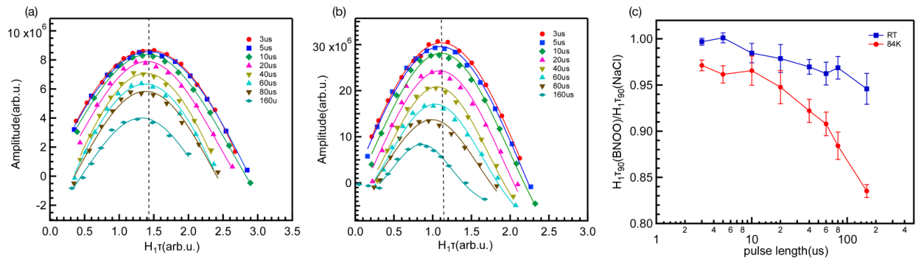
Fig.6.6 shows an optimal pulse condition experiment to see whether the optimal pulse condition changes when the pulse lengths are increasing. As mentioned in section 3.2.1, the frequency window of a certain square pulse is inverse proportional to the pulse length. So increasing the NMR pulse length will restrict the available excitation range in the frequency domain and can be used to irradiate selective regions in the NMR spectrum. For I=3/2 nuclei with quadrupolar splitting, the optimal pulse strength to irradiate the central line is only half of that to irradiate all lines[63], so by increasing the pulse lengths, if there is any quadrupolar noise, the optimal pulse strength will decrease. Otherwise, the optimal pulse strength should stay at 1 and keeps the same value with the increase in pulse length. In experiments, the pulse strength depends both on the pulse lengths and the attenuation level of the output voltage and can be characterized as
| (6.4) |
with an arbitrary unit. The H1 represents the excitation oscillating magnetic field and is the pulse length in , Tx is the attenuation of the output voltage and can take values such as -1dB, -2dB, etc. Calibration of the attenuators and the linearity of the RF power amplifier need to be carried out before applying this approach on the single crystal Ba2NaOsO6. Here we take NaCl single crystal (which is a perfect fcc without any quadrupolar effect) as the reference sample and measured the optimal pulse strength by varying the level of attenuation at a constant pulse length, respectively at room temperature and 84K due to their different T1 values. The same measurements were done on the single crystal Ba2NaOsO6 and the optimal pulse condition was adjusted based on the corresponding calibrated NaCl results at a certain attenuation level. The vertical dotted line in Fig.6.6(a) and (b) indicates the optimal pulse strength for Ba2NaOsO6 single crystal after NaCl calibration at room temperature and 84K respectively. We can see the shift of the optimal pulse condition to a smaller value with the increase in pulse lengths. And we plot the ratio of the optimal pulse strength between single crystal Ba2NaOsO6 and NaCl, we see from Fig.6.6 (c) that with the increase of pulse lengths, the ratio drops below 1 and drops more profoundly for the 84K case. This indicates the presence of quadrupolar noise at both 84K and room temperature, providing additional evidence for the argument we make earlier.
6.1.2Broken local point symmetry phase
The above study will have potential application in studying a possible ”spin-nematic” (quadrupolar) phase when the system just enters into the ”broken local point symmetry” phase and no clear quadrupolar splitting has yet developed. Fig.6.7 and Fig. 6.8 show the angle dependence measurements at the temperature close to the possible ”spin-nematic” phase temperatures from 4T to 33T. One can see that the behavior at low field and high field are quite different, and at the magic angle position of 4T, the spectrum shows as a bump without any discernable peak. The multi-modal quadrupolar spectroscopy as discussed in the above section might be applied to address questions such as what are the quadrupolar interaction parameters in this situation and the nature of the possible ”spin-nematic” phase.


6.2 Ba2LiOsO6
We have reviewed the earlier experiments on Ba2LiOsO6 in Chapter 2 section 2.1.3. In the following subsection, we will present the NMR results of Ba2LiOsO6[102, 103], which differs from its isostructural isovalent compound Ba2NaOsO6, indicating the sensitivity of the magnetic ground state to the delicate change of interactions strength in the osmate 5d1 double perovskite system. Fig.6.9 shows the single crystal field cooled (FC) susceptibility at low field (0.5T) and high field (9T) along the three high symmetry axes [001], [110] and [111]. We see that the susceptibility measurements show a magnetic transition happens at around 5K. This is a little different from the earlier experiment carried on powder [40] as shown in Fig. 2.4 (a), which reveals the cusp like AFM transition at 8K. However, our results are consistent with the most recent characterization of double perovskite containing 5d1 transition metal ions [12], which shows that the susceptibility of Ba2LiOsO6 does not have a clear cusp at 5K and the FC and zero field-cooled (ZFC) has minimum divergence. One possible reason is that since both here and Ref. [12] were using single crystal and the AFM staggered direction is not aligned with any of the measurements, while was picked up by the powder measurements.
Given the high-temperature NMR shift and the susceptibility values, we can obtain the Clogston-Jaccarino plot with temperature as an implicit parameter, as shown in Fig.6.10. The hyperfine tensor constant and the temperature-independent shift can be extracted from the slope and interception values of a linear fit. Details of the derivation can be found in Ref [99]. We can then obtain that the hyperfine coupling tensor constant and the NMR orbital shift is 0.0408. 11 1 We need to note that if we express the hyperfine tensor in unit of , then the unitless shift will have unit of . 1 emu=1.07810 and 1 mole=NA=6.02. So and the hyperfine tensor constant is the slope value divided by 0.18, which equals to 0.185. Hyperfine tensor unit is usually reported as or . The hyperfine coupling tensor value is much smaller than that in Ba2NaOsO6, which is [99]. Furthermore, the electric quadrupole moment for Ba2LiOsO6 (oblate) is also of that of Ba2NaOsO6 (prolate). This means that even if the physics happens at the 5d1 Os site in Ba2LiOsO6 is of the same magnitude as that in Ba2NaOsO6, NMR on Li for Ba2LiOsO6 is less sensitive than NMR on Na for Ba2NaOsO6 regarding both the hyperfine interaction and the electric quadrupolar interaction.

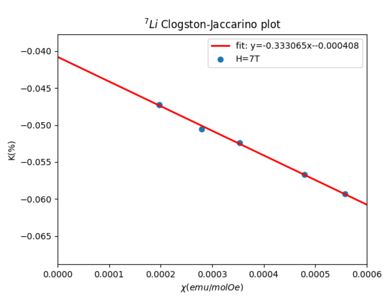
6.2.1NMR spectrum
Fig. 6.11 shows the NMR spectrum below (3.3T) and above (13T) the metamagnetic transition at 5.75T. The corresponding shift obtained by peak position and first moment are shown in Fig.6.12. We can see that albeit the AFM order it is supposed to be at low temperatures, no discernible spectrum splitting has been observed. The high field spectrum develops an obvious unsymmetric shape while the low field spectrum is symmetric down to the lowest temperature. The shift analysis has shown that below the metamagnetic transition, there is a cusp at the magnetic transition temperature TN while above the metamagnetic transition, the shift keeps almost constant with a gradual increase in magnitude. For a typical 3D antiferromagnet, susceptibility perpendicular to external magnetic field is larger than the susceptibility parallel to external magnetic field , with the former showing a constant value below TN and the latter shows a cusp at TN [104]. Since the Knight shift is proportional to the local susceptibility , the different behavior of shift below and above the metamagnetic transition suggests that the transition should be a first-order spin-flop transition [104].


This spin-flop transition can also be seen from the sudden change of spectrum shape and the discontinuity in the linewidth as shown in Fig.6.13. Fig.6.13(a) is at 4.3K. We can see that the spectrum undergoes a sudden change of shape from almost symmetric to unsymmetric when crossing the spin-flop transition from 5.75T to 6T. To make a comparison with the case of Ba2NaOsO6, the 6T spectrum has been fitted by a second magnetic shoulder peak and a triplet of quadrupolar splitting peaks to show the how multiple peaks can be resolved in this case. Fig.6.13 (b) shows that the full width at half maximum (FWHM) experiences a sudden jump going from 5.75T to 6T. The experimental FWHM value and the FWHM value extracted from spectrum fitting with Gaussian, Lorentzian, and Voigt functions have all been shown in Fig.6.13 (b). We can fit the FWHM magnetic field in the region out of the vicinity of the metamagnetic transition (the red points in Fig.6.13(c)) with a linear function. Then we can get Fig. 6.13(d) divided by the slope of the line. We see that when the FWHM is scaled by field, what happens at the spin-flop transition is a gradual decrease of scaled FWHM before the on-site of this first-order transition. There are two possibilities for the decrease of scaled FWHM. One is due to possible motional narrowing, where the increased fluctuation of magnetic moments before the spin-flop transition causes a reduced distribution of time-averaged local magnetic field as experienced at the nuclei sites, resulting in a reduced linewidth. The second possibility is that before the on-site spin-flop transition, the antiparallel arranged spins with the staggered direction along the external field direction have already started to tilt away from the field direction, resulting in a reduced staggered local field along the external field direction, which is what is reflected by the linewidth. Currently, there is no further evidence to show which possibility is the more probable one.
6.2.2Spin-lattice relaxation rate and spin-spin relaxation rate
Fig.6.14 shows the spin-lattice relaxation rate results for Ba2LiOsO6. The T1 values are extracted from stretched exponential decay. As seen in the inset of Fig.6.14, the spin-lattice relaxation rate has a divergence behavior at the magnetic transition temperature TN with a high-temperature shoulder at around 100K. The spin-lattice relaxation rate below the magnetic transition can be fitted with the Raman (two-magnon, one in and one out of the scattering) process [105]
| (6.5) |
where D is the dimension of the system. Constraint fitting with D=2 and D=3 indicates that the system is compatible with a 3D case as shown in Fig.6.14 (a). Fig. 6.14 (b) illustrates the temperature dependence of the stretched exponent , which indicates the development of distribution of T1 starting from around 20K, consistent with the onset of peak, where starts to increase. The field dependence and angle dependence of below magnetic transition are shown in Fig.6.14 (c) and (d), where the stronger magnetic field freezes magnetic fluctuation and suppresses [106], and the angle dependence measurements show oscillation behavior as expected for the antiferromagnetic case with Raman relaxation process [107].


Fig.6.15 shows the spin-spin relaxation rate below and above the metamagnetic transition field 5.75T. The spin-spin relaxation time T2 is extracted from stretched exponential decay. The behavior below and above the spin-flop transition is very different for these two scenarios. We also need to note that the T2 decay curve can be very sensitive to the pulse sequence (such as 90-90 or 90-180 echos) and the pulse lengths. Further theoretical work needs to be done to understand better the behavior in this sample. We have consistently observed a bump above the magnetic transition, especially obvious for the case above spin-flop transition as shown in Fig.6.15 (b), which might be related to orbital fluctuations.
6.3 Ba2NaxCa1-xOsO6
6.3.1Introduction
In this subsection, we will extend the study from 5d1 material to doped 5d1 compounds to explore the effect of charge doping on the double perovskite Ba2NaOsO6. We will focus on understanding the structural and magnetic transitions from the NMR spectrum on a series of charge doping compounds of Ba2NaxCa1-xOsO6 through the Na+/Ca++ partial substitution for 0 x 1. We find that all the doped samples remain magnetic insulators despite the added electrons. Moreover, similar to Ba2NaOsO6, before the onset of magnetic ordering, there is an intermediate temperature region with orthorhombic electric field gradient (EFG) symmetry, indicating a breaking local point symmetry (BLPS) phase. For the low-temperature magnetic state, the ferromagnetic moment component is almost completely suppressed when 0.125. Under the canted AFM model for Ba2NaOsO6, the staggered angle is around 86(1) degrees for 0.1250.9, implying a collinear AFM state. The Jahn-Teller type structural transition indicates the existence of possible quadrupolar moments. However, our current NMR experiments (with also complementary sR measurements[108]) are not able to distinguish multipolar orders. Whether there are multipolar orders when the system evolves from a cAFM 5d1 Ba2NaOsO6 to a ferro-octupolar 5d2 Ba2CaOsO6 needs further experimental evidence. In the following subsections, we will first describe the powder NMR spectrum fitting for the intermediate temperature ”BLPS” phase and then present a powder NMR spectrum simulation that is based on the canted AFM model used to describe the Ca0 Ba2NaOsO6[41].
6.3.2Powder NMR spectrum fitting for intermediate temperature ”BLPS” phase
The series of 5d1 charge doping samples Ba2NaxCa1-xOsO6 (0 x 1) has been measured by sR and NMR[108, 109]. The magnetic transition temperatures Tm have been determined from zero-field muon spin relaxation as the onset (5) of magnetization volume. Bifurcations of the NMR spectrum’s first moment and peak positions have been observed in all the doping samples, suggesting that the spectrum starts to develop unsymmetry above the magnetic transition temperature TN, which is determined from the bifurcation point from 1/ (K is the Knight shift) plot in NMR measurement. The intermediate temperature range refers to the temperature range of Tm T Tn.
The powder spectrum fitting is based on the code in Ref [110]. The fitting parameters are manually adjusted based on the following constraints for three different symmetries of EFG as shown below in Table 6.1.
| Symmetry | Vzz | Hyperfine shift() | |
| Cubic | =0 | =0 | Kx=Ky=Kz |
| Tetragonal | 0 | =0 | Kx=Ky |
| Orthorhombic | 0 | 0 | |
Fig.6.16 shows the best fitting results for the three symmetries at the intermediate temperature region for the doping samples from Ca0 to Ca50 at 11T. The difference between the data spectrum (blue solid line) and the fitted spectrum (red filled shape) is characterized by the deviation as calculated by , where f is the fitted spectrum and g is the data spectrum. The fitted spectrum f is generated with the same range and the same number of frequency points n as the data spectrum g. For all the Ca doping concentrations, the orthorhombic case has the smallest deviation (Fig.6.17), suggesting the orthorhombic structural distortion. Another independent powder spectrum simulation for these intermediate temperature spectrums has also confirmed the result[111].

6.3.3Powder NMR spectrum simulation for low temperature magnetic state based on colinear canted AFM model
Simulation model
Powder spectrum simulation based on a two sublattice canted antiferromagnetic order model of Ba2NaOsO6 single crystal was performed to study how doping might change the spin staggered arrangement. This simulation is constructed by using a two sublattice spin staggered pattern (similar to the one used for Ba2NaOsO6(BNOO) single crystal, refer to Ref.[41]) and calculating the local field distribution at two distinct Na sites when the sample is oriented at an arbitrary angle relative to the external field direction according to , where is the hyperfine coupling tensor (in T/) and is the local spin moments (in ). The local fields (in T) generated by quadrupolar effects are then added using fixed EFG parameters obtained from intermediate temperature spectrum fittings. The combined local fields are then plotted in a histogram and then convoluted with a Gaussian function to get the final simulated spectrum (in MHz) to compare with the data.
One can see that from the way this spectrum simulation is constructed, several factors are very important to get the correct results, such as what is the spin arrangement and net/effective moment when the field is at an arbitrary angle relative to the sample, the hyperfine tensor values, etc. Below we discuss in detail how these factors are considered in the simulation.
Spin staggered pattern The spin directions for this simulation are based on the BNOO single crystal’s inplane canted AFM [110] pattern[41]. Sublattices A and B are staggered by approximately 67 degrees relative to the easy axis [110] on two neighboring layers. And based on the diagonal rotation pattern of BNOO, the two sublattices of spins rotate with the field direction on the same plane while keeping the same staggered angles when the field direction is rotated from [110] to [001].
Extending to the powder cases, the field dependence of the spin sublattice directions is assumed to be the same as in the case for BNOO single crystal for the all 4 solid angle, not only when the field direction is along with the diagonal rotation directions but also when the field is rotated on the plane. This means that the staggered spins keep the same staggered angle relative to the field direction when they are placed in different orientations relative to the external field.
Field dependence of net moment from BNOO single crystal
There is very important information that is needed to be able to fit the diagonal rotation pattern of averaged field and staggered field for BNOO in Ref[41]. This is the field dependence of net moment on single-crystal BNOO, refer to Figure 3 on Ref[39]. Since we don’t have this information for the doped powder sample though, the same angle dependence of net moment is used for all the doped powder samples based on their effective moment values, which will be described in the next paragraph.
Effective moment values
For the BNOO single crystal, the effective moment is 0.6. The same is obtained for the BNOO powder sample. So the effective moment for all the doped samples in the simulation is taken as the effective moments obtained from susceptibility measurement. These effective moments are used in combination with the field dependence of the net moment as described in the paragraph above.
Hyperfine tensor
The initial values for the diagonal components of the hyperfine coupling tensor are set based on the values obtained from Clogston-Jaccarino plots for all the doping concentrationsFor the off-diagonal values, the symmetry of the tensor is taken as the one obtained for BNOO single crystal in Ref [41]. The tensor form is = .
Quadrupolar effect
The quadrupolar effect is added to the two distinct Na sites after obtaining their local field from . The EFG parameters and principle axes are fixed, taken from the values fromthe intermediate temperature results. The corresponding local fields generated from quadrupolar splitting is written as , where and describes the orientation of external field relative to the EFG principal axes. These quadrupolar local fields are combined with the local field generated from hyperfine interactions to obtain the local field histogram in the unit of MHz.
Results
Fig. 6.18 shows the optimization results for all doping concentrations. The optimization solver used in Python is “Nelder-Mead”. All the spectrums are first manually tuned to the closest match to the data spectrum with fixed parameters as mentioned above. In the plots below, the histograms are plotted in blue and the orange line represents the generated spectrum after being convoluted with a Gaussian function. Both simulated (in orange) and data spectrum (in green) are normalized by amplitude.
Simulation results with the comparison with data are shown in Fig.6.19. The simulation results show that staggered angle changes from 68 degree to nearly 90 degree AFM cases with the increasing Ca doping. This can explain the doping dependence on the Knight shift. (The staggered angle determined the first moment of the spectrum.) As we can see for the Ca90%, the Gaussian blur increased a lot for the Ca90% spectrum to be able to fit its large linewidth. However, the calculated local field distribution as plotted in the histogram does not increase a lot. This indicates that there might be other sources to be counted for the large linewidth at Ca90%, especially considering the Ca100% has been claimed to have octupolar order rather than Neel order. The physics for Ca90% might also be different from the current two sublattices staggered spin model.

Since the current model treats the effective moments of all the doping samples as fixed input parameters, the current calculated Knight shift, and linewidth from the simulated spectrum are compatible with their effective moments. The decrease of Knight shift from Ca0% to Ca12.5% is because of the staggered angle changes from 67 degree to 85 degree. And the decrease of linewidth from Ca0% to Ca 25% can be accounted for by the decrease of the off-diagonal components for their hyperfine coupling tensor, even though the effective moments are increasing in this region. Above Ca25% doping, the off-diagonal components are about constant up to Ca90%, and the increase of linewidth in this region comes from the increase of the effective moments.

While completing the thesis, we have been aware of many recent theoretical studies on the 5d2 compounds[112, 18, 16, 15, 17], claiming ferro-octupolar or antifero-quadrupolar ordering for the materials like Ba2CaOsO6. We note that our current NMR study on the 5d1 electron-doped powder is not able to determine the multipolar ordering. That being said, based on the fact that all the doped powder samples have shown orthorhombic local distortions at intermediate temperatures, there should be quadrupolar moments existing in the compounds. This is probably due to strain in the lattice caused by partially replacing Na+ with Ca2+ ions.
| Ca | , () | |||
| , | ||||
6.3.4Summary
In summary, we studied the effect of electron doping on 5d1 Mott insulator Ba2NaOsO6 by sR and NMR spectroscopy on powder compounds Ba2Na(1-x)CaxOsO6 (0x0.9). For all doping samples, no insulator to metal transition has been observed and all samples remain as magnetic insulators. We found that the ferromagnetic moment component in Ba2NaOsO6 is suppressed by doping[113, 108, 114]. Based on the two sublattices staggered model for Ba2NaOsO6, we found the magnetic ground state of doping samples (0.125x0.9) can be modeled by a collinear AFM case with staggered angle around 86(1) degree. Moreover, we found that similar to the 5d1 Ba2NaOsO6 case, there are intermediate temperature orthorhombic structural distortions for all doping samples. The structural and magnetic phase transition temperatures increase monotonically with doping. While preparing for this thesis, we have been aware of many recent theoretical papers on the multipolar ordering for 5d2 Mott insulators, we need to note that the current NMR powder experiments are not able to directly probe multipolar ordering. The fact that there are orthorhombic structural distortions in these doped samples indicates the possible existence of quadrupolar moments. The associated Jahn-Teller type of local distortion might be induced by strain in the lattice when replacing Na+ with Ca2+ ions. However, whether there are ferro-quadrupolar ordering ground states or other multipolar ordering in the doped samples when the system evolves from a cAFM 5d1 Ba2NaOsO6 to a ferro-octupolar 5d2 Ba2CaOsO6 is still unclear and need to be studied further by future experiments, such as synchronized x-ray spectroscopy. Nevertheless, by investigating the doping effect on the evolution of the magnetic and structural phases, this work started a new path in the current research of understanding the complex interplay of magnetic, structural, and lattice degree of freedom for the interesting 5d1 and 5d2 Mott insulator system.
CHAPTER 7NMR study on mixed valence insulator SmB6
In this chapter, we will focus on a completely different materials system other than the double perovskite magnetic Mott insulator that we have been studying in the previous several chapters. We will describe the NMR study on a mixed-valence insulator SmB6. Owing to strong electronic correlations, SmB6 is a Kondo insulator that has been studied for several decades[115] and has more recently been proposed to be a topological Kondo insulator[116]. Recent magnetic torque measurements on pristine floating-zone grown single crystals of SmB6 found bulk quantum oscillations despite the bulk electrical insulating behavior[117], suggesting the surprising existence of a bulk Fermi surface in this unconventional insulator. We have conducted NMR measurements on the same high-quality floating zone grown single crystals of SmB6 below 1K and for magnetic fields up to 18T for two inequivalent boron sites B1 and B2. For all magnetic fields below 18T, the Knight shift remains constant below 1K, showing behavior akin to a bulk metal, despite the bulk electric insulating character of the material. The spin-lattice relaxation rate 1/T1 indicates the existence of localized fermion density of states at low fields while showing constant behavior above 6.6T. The anisotropy of the spin-lattice relaxation rate is suppressed with the increase of the magnetic field and disappears when approaching 18T. The Korringa constant indicates the presence of antiferromagnetic correlations to ferromagnetic correlation with an increase in the magnetic field. We found that with the physical constraints that need to be considered for the two inequivalent boron sites, our data can not be explained by the in-gap state model[118], which implies the possibility of the existence of a neutral bulk Fermi surface.
7.1 Introduction
Samarium hexaboride has been studied for several decades and it is initially characterized as a Kondo insulator[115]. Kondo insulator describes a group of materials that opens a small band gap at low temperature due to the hybridization of localized electrons with conduction electrons. In SmB6, the 5-10 meV band gap is opened because of the localized 4f and itinerate 5d electrons hybridization and strong correlation. In recent years theoretical works propose that it might be a topological Kondo insulator[116], having an insulating bulk and a conduction surface state that is protected by the crystal point symmetry. Evidence for this topological surface states have been observed by ARPES[119], tunneling spectra[120] and quantum oscillations[121]. However, there are still some mysteries about this material. Especially on the observation of quantum oscillation on magnetic torque[117] coming from the bulk and also some inconsistent and conflicting results for this material based on different growing methods. To explain mainly the quantum oscillation in the bulk along with other properties such as specific heat and thermal conductivity, a lot of theoretical works have been done.
These theoretical works can mainly be divided into two groups. One is trying to explain the bulk quantum oscillation from the extrinsic origin, such as in-gap states induced by disorder[122], lattice defects[123], donors and acceptors’ impurities[124], isolated local magnetic moment[125] or topological non magnetic impurities[126], etc. The other group is trying to look into some possible intrinsic origin, such as itinerate electrons coupled to the flat band in the absence of a fermi surface[127], ”Skyrme insulator” with Majorana fermi surface[128], Boson exciton with a small gap and finite-Q dispersion minimum[129], neutral quasiparticles in the bulk that forms the fermi surface[130], and Majorana fermi band that breaks gauge symmetry[131], etc. To address whether the quantum oscillation comes from extrinsic or intrinsic origins, in this chapter we have used NMR to study the unconventional fermi surface in the bulk using the same sample that the bulk quantum oscillation has been observed[117].
There have been three prior studies of using NMR in studying the single crystal of SmB6, two of them using samples flux-grown samples[132, 118], the other one uses floating zone grown sample [133]. While the high temperature (above 15K) NMR spin-lattice relaxation rate follows the gap excitation behavior and is field independent, which shows consistency among the three studies, the low temperature (below 15K) 1/T1 differs based on different growing methods. For flux-grown samples, there is an anomaly local maximum on 1/T1 at low field, which is attributed to the fluctuation of ”remagnetized” Sm3+ ions near Sm-site vacancies in Ref.[132], and by the presence of the in-gap state in Ref.[118]. For floating zone grown sample[133], an increase of 1/T1 with the decrease of temperature was observed from 6K to 10K followed by a constant 1/T1 down to 4.2K. This indicates the existence of some low-energy magnetic excitation that is not a local moment associated with magnetic impurities. In this study[134], our NMR spin-lattice relaxation rate is compatible with the earlier floating zone grown sample above 4.2K (See Fig.7.6(b)) and beyond that, we extend the measurement done the 60mK lowest and up to 18T. We also measured the 1/T1 for two inequivalent boron sites showing anisotropy of this fluctuation is suppressed by the magnetic field.
7.2 Methods
7.2.1Sample preparation
High-quality single crystals of SmB6 were grown using the floating zone method, as described elsewhere [117]. NMR measurements were performed for a single crystal with a volume of approximately 1 mm3. The quality of the sample was confirmed by the sharpness of 11B and the clean baseline of NMR spectra. The sample was both zero-field and field-cooled. We did not detect any influence of the samples cooling history on the NMR spectra. Nevertheless, for consistency, all results presented in the thesis were obtained in field-cooled conditions. The sample was mounted on the plane, with an external field parallel to the axis. For measurements at Brown University, the sample was mounted to a GaAs/Sapphire substrate, with four thermal insulation spacers made of Vespel in a pyramid shape that is higher than the thickness of the sample and attached to both sides of the substrate as shown in Fig.7.1. This is to make sure that even in the case that the solenoid coil around accidentally moves, it will only have contact with the Vespel spacer and will not have contact directly with the sample so that the sample will not be heated up from pulsing. The solenoid coil also had a cross-sectional area significantly larger than that of the sample with substrate and Vespel spacer. Then the substrate is clamped by a copper sample holder that is thermally anchored to the cold finger to ensure that the sample will have the sample temperature with the cold finger.

7.2.2NMR measurements
The measurements were done at Brown University for magnetic fields up to 10 T and at the NHMFL in Tallahassee, FL
at higher fields. In both laboratories, high homogeneity superconducting magnets were used.
The temperature control was provided by 4He variable temperature insert.
The NMR data were recorded using a state-of-the-art laboratory-made NMR spectrometer. The spectra were obtained, at each given value of the applied field, from the sum of spin-echo Fourier transforms recorded at constant frequency intervals. We used a standard spin-echo sequence . The shape of the spectra presented in the manuscript is independent of the duration of time interval . Since nuclear spin of 11B equals and both B sites (B1 and B2) are in non-cubic environments, three distinct quadrupolar satellite lines are observed per site [49].
The shift was obtained from the frequency of the central transition using a gyromagnetic ratio of = 13.6552 MHz/T. The same gyromagnetic ratio was used for all frequency to field-scale conversions.
7.3 Results
7.3.1NMR spectrum
The NMR spectrum of 11B is illustrated in the inset of Fig.7.2. With the external applied magnetic field, the boron sites have two inequivalent sites B1 and B2. B1 are boron sites that are along the applied field direction while B2 is on the plane that is perpendicular to the external field direction. Firstly we found that for all the magnetic fields from 5T to 18T, the Knight shift below 1K is constant (see Fig.7.6(a)), indicating metallic behavior. As for the field dependence, there is a slight increase of the Knight shift with the increase of magnetic field as shown in Fig.7.5(b).
7.3.2Spin lattice relaxation rate 1/T1
The NMR spin-lattice relaxation rate was measured on the transition on both boron sites using a series of comb pulses as saturation pulses. The T1 values are obtained by fitting the saturation recovery curve to the standard recovery profile for the satellite of nuclei with using the comb pulses saturation method and assuming purely magnetic relaxation as shown below.
| (7.1) |
T1 value is extracted from this formula with the stretched exponent set to 1. This is justified by comparing fittings using stretched and non-stretched equations for both sites at 5T and 18T. The best fits all come from the non-stretched fits, indicating that there are no inhomogeneous/glassy features for the sample. Selective fittings as an example can be found in Fig.7.3 Using purely quadrupolar relaxation or mixed magnetic and quadrupolar relaxation gives the same temperature dependence on the spin-lattice relaxation rate.
Below 1K, for both B1 and B2 sites, the 1/T1 decreases linearly in temperature above 6.6T (Fig.7.2(a)), which can be seen more clearly from the 1/(T1T) plot in Fig.7.2(b), showing the constant behavior, indicating a metallic Fermi surface. Below 6.6T though, we have observed a local enhancement of the density of states as shown in the bump in 1/(T1T). Also if we look at the 1/(T1T) versus the magnetic field, we can see that the B2 sites which are in the plane perpendicular to the external magnetic field experience a higher density of states but the anisotropy between these two sites is suppressed by the increase of magnetic field (Fig.7.5(a)). We can also look in more detail at the local enhancement of density of states happening in the low field region. We see for both sites, the enhancement happens at around 500mK (Fig.7.4). Combining the shift and 1/T1T result we can look at the Korringa product in Fig.7.5(c)and (d).

According to Korringa relation , where is the Knight shift K, is the electron gyromagnetic ratio, is the nuclear gyromagnetic ratio, the Korringa product is defined as . So the reciprocal of Korringa constant for non interacting Fermi gas is . Plug in the values, (or ), (or for 11B according to NMR periodic table. Then
| (7.2) |
For the calculation of , the Knight shift K is taken as the shift between the central peak and the natural frequency position for the two 11 B sites. Since the quadrupolar splitting is roughly the same in the range of fields we studied, this shift value K is also the shift for the rightmost satellite, on which the T1 measurements are taken.

We see that for fields above 6.6T the Korringa ratio is constant, indicating a metallic fermi surface state. The absolute value of the Korringa ratio decreases with increasing magnetic field, going from favoring antiferromagnetic fluctuation to favoring ferromagnetic fluctuation. Due to a much smaller Knight shift for the B2 sites, the Korringa product for B2 sites is much larger than that for B1, which is also associated with a very large error bar. These results can be found in the supplement Fig.7.6(c) and (d).
7.4 Discussion
The enhancement of 1/T1 at low magnetic fields has earlier been discussed in terms of an in-gap state model[118]. Since we have measured both the B1 and B2 sites, there are extra physical constraints that need to be satisfied. Firstly, the position of the band edges for the conduction and in-gap state bands should be the same although they might be field dependent. Secondly, the area of the conduction and in-gap state bands, which represents the total density of states, should be field independent although they might differ between the two boron sites. Upon applying these constraints to our fitting of the 1/T1 temperature dependence, we found that the in-gap state model is not able to describe our data, especially for the local enhancement of the density of states at low fields. We, therefore, suggest that the bulk metallic surface state is coming from other intrinsic origins beyond the in-gap state model.
CHAPTER 8Conclusion
In this thesis, through a comprehensive effort on theoretical model simulation, first principle calculation, and NMR experiments, we have gained valuable new understandings of the 5d osmate double perovskite system. In particular, we answered some very interesting questions related to the 5d1 double perovskite Mott insulator Ba2NaOsO6 and we will summarize our findings for each project as below.
One significant contribution we have made is about the origin of the missing entropy in the single crystal Ba2NaOsO6. Chapter 6 section 6.1 showed that we have observed oscillation-like ”plateau” behavior in the spin-spin relaxation rate T measurement using standard spin-echo sequence above the structural transition temperature of Ba2NaOsO6. Unlike the well-known oscillation of spin-echo amplitude as a function of the spacing between the 90 and 180 pulses in linear scale in the presence of clear quadrupolar splitting, we have observed a ”plateau” in the T2 decay profile when is put in logarithmic scale. And based on the simulation of multi-modal quantum spectroscopy to characterize quadrupolar noise, we found that the ”plateau” decay curves fit well with the model when there is a non-zero Lorentzian distribution of quadrupolar noise with the average value of . The width of the Lorentzian distribution shows divergent behavior, and the asymmetry factor becomes non-zero and keeps increasing toward 1 when the system is approaching structural transition temperature. The non-zero distribution persists up to at least 50K, above which the thermal effect starts to set in and causes level mixing between the Sz= and Sz= states, preventing an accurate extraction of the value from the fitting above this temperature. The results indicate that there are domains in Ba2NaOsO6 with different Lorentzian distributions of above the structural transition and that is where the remaining entropy lies. Details of the dynamics of these quadrupolar domains can be further studied by the CPMG sequence.
Another interesting physics we have learned is from the first-principle calculation of the electric field gradient tensor in Ba2NaOsO6 shown in Chapter 5 section 5.2, and the Monte Carlo simulation on the 5d1 double perovskite model with strong spin-orbit coupling in Chapter 4. In the EFG calculation project, we found that the strong spin-orbit-coupling is not large enough to induce the non-zero electric field gradient value that is obtained from NMR measurements. Instead, the actual displacement of oxygen atoms in the Na-O octahedra is needed to produce the measured EFG parameters. In particular, the distortion involves elongation and compression of the oxygen atoms along crystal axis a and c for (0.53%-0.55% of the Na-O bond length) respectively while the oxygen atom along the b axis remains at the non-distorted position. This is a Q2 type of distortion of the Na-O octahedra and corresponds to the antiferro-quadrupolar moment . For another 5d1 compound Ba2MgReO6, synchrotron x-ray experiments found that in the proposed phase, the Re-O octahedra distortion can be decomposed into a linear combination of the two normal modes of an octahedron Q3 and Q2. These two modes couple to the two quadrupolar moments and respectively. And these two quadrupolar moments form the two-dimensional group which is analogous to the eg orbital of 3d electron. However, mean-field calculation on the 5d1 model with strong spin-orbit-coupling only shows a single non-zero quadrupolar moment in the quadrupolar ordering state. To reconcile the discrepancy between experiment and theory, we carried out a classical Monte Carlo simulation on the same model. We found that in the pure quadrupolar case when only the coupling constant of the electric quadrupolar interaction term is non-zero, the quadrupolar state is characterized by two non-zero quadrupolar moments and . This also happens when there are non-zero magnetic coupling constants and the quadrupolar state occurs at the intermediate temperature region, which is consistent with the experiment on Ba2MgReO6. While for the mean-field treatment considering 2 sites per unit cell, the combination of C4 rotation about the axis and a translation exchanging A and B sublattices remains a symmetry for the quadrupolar state, this symmetry is broken in the Monte Carlo simulation considering 4 sites per unit cell. And this additional symmetry breaking gives rise to the non-zero ferroic quadrupolar moment observed in experiments. From this Monte Carlo simulation, we also showed that the coplanar canted FM[110] state is a unique quantum state that does not have a correspondence on a classical basis. Our first-principle calculation on the magnetic and orbital order for Ba2NaOsO6 is presented in Chapter 5 section 5.3. Here we found that the staggered orbital ordering coexists with the cFM order. This is characterized by two sublattice spin densities and different selective occupations of d orbitals for the two sublattice Os ions. Furthermore, our results affirm that multipolar spin interactions are an essential ingredient of quantum theories of magnetism in SOC materials.
Besides Ba2NaOsO6, we have also studied its isostructural isovalent compound Ba2Li-
OsO6 in Chapter 6 section 6.2. We found that although characterized by susceptibility measurements as an antiferromagnet, the NMR spectrum does not show any splitting below its magnetic transition temperature and only significant line broadening has been observed. The spectrum shape has a sudden change from symmetric to unsymmetric while crossing the metamagnetic transition field Hc=5.75T. The linewidth scaled by magnetic field has a sudden jump right at the transition field Hc, indicating a first-order transition. It also shows a gradual decrease when the field is increasing and approaching Hc, possibly related to motional narrowing of the spectrum. The shift and first moment in the ordered state below and above Hc shows that the metamagnetic transition is a possible spin-flop transition. The fitting of the spin-lattice relaxation rate T indicates that the ordered state is more likely to be a 3D antiferromagnet. The spin-spin relaxation rate T shows enhancement above magnetic transition temperature 5K, which might be related to orbital fluctuation and requires further study in the future. In Chapter 6 section 6.3 we study the electron doping effect on 5d1 compound Ba2NaOsO6. We carried out NMR and sR experiment on powder sample Ba2NaxCa1-xOsO6 (0x1) and constructed the magnetic and structural phase diagram as a function of doping. We found that albeit with added electrons, all samples remain as magnetic insulators, indicating the existence of a charge trapping mechanism which has been shown recently by DFT calculation to be the possible formation of small polarons, which are quasiparticles that couple excess charge with lattice vibration[135]. This leads to a localized charge distribution around Os ion sites for the Ca12.5% compound. The NMR spectrum develops an unsymmetric shape at temperatures above magnetic transition, which based on powder spectrum simulation is due to a similar ”broken local point symmetry” phase with orthorhombic EFG symmetry. The spectrum at the low-temperature magnetic phase has been simulated based on a collinear two-sublattice AFM model and we found that the staggered angle goes from 67 degrees to close to 90 degrees relative to the easy axis [110] with the increase of Ca doping, which indicates that under this model, the system goes from a canted ferromagnetic order to a collinear AFM order with Ca doping. That said, we can not exclude the existence of possible ferro-quadrupolar ordering or other multipolar ordering in these doped samples, and it still needs further experiments, such as synchronized x-ray spectroscopy, to study in more detail. In the end, in Chapter 7, we report the spin-lattice relaxation rate measurement on mixed-valence insulator SmB6. We have conducted NMR measurements on high-quality floating-zone grown single-crystal SmB6 below 1K and up to 18T for two structurally distinct boron sites. Our highly resolved NMR spectrum and non-stretched recovery fits have demonstrated a high-quality clean sample, excluding our observation of impurities effects. Our high-temperature results above 1K are consistent with the earlier results on floating-zone grown SmB6. Below 1K, we have observed constant Knight shift and 1/ (T1T) behavior above 5.5T, indicating a metallic Fermi surface. Our result is not compatible with the in-gap state model and a new theory is needed to understand the unconventional fermi surface. In conclusion, focusing on the 5d osmate double perovskite system, this thesis has provided a valuable new understanding of the fundamental properties of these transition metal compounds, which also promotes the development of the NMR quadrupolar noise spectroscopy with possible future application in other material system.
Bibliography
- [1] William Witczak-Krempa, Gang Chen, Yong Kim and Leon Balents “Correlated Quantum Phenomena in the Strong Spin-Orbit Regime” In Annual Review of Condensed Matter Physics 5.1, 2014, pp. 57–82 DOI: 10.1146/annurev-conmatphys-020911-125138
- [2] Michi-To Suzuki, Hiroaki Ikeda and Peter Oppeneer “First-principles theory of magnetic multipoles in condensed matter systems” In Journal of the Physical Society of Japan 87.4 The Physical Society of Japan, 2018, pp. 041008
- [3] Leonid Pourovskii and Sergii Khmelevskyi “Hidden order and multipolar exchange striction in a correlated f-electron system” In Proceedings of the National Academy of Sciences 118.14 National Acad Sciences, 2021
- [4] Tomohiro Takayama et al. “Spin–Orbit-Entangled Electronic Phases in 4d and 5d Transition-Metal Compounds” In Journal of the Physical Society of Japan 90.6 The Physical Society of Japan, 2021, pp. 062001
- [5] Daigorou Hirai and Zenji Hiroi “Successive Symmetry Breaking in a Jeff= 3/2 Quartet in the Spin-Orbit Coupled Insulator Ba2MgReO6” In Journal of the Physical Society of Japan 88.6 The Physical Society of Japan, 2019, pp. 064712
- [6] Daigorou Hirai et al. “Detection of multipolar orders in the spin-orbit-coupled Mott insulator ” In Phys. Rev. Research 2 American Physical Society, 2020, pp. 022063 DOI: 10.1103/PhysRevResearch.2.022063
- [7] SW Lovesey and DD Khalyavin “Magnetic order and 5d1 multipoles in a rhenate double perovskite Ba2MgReO6” In Physical Review B 103.23 APS, 2021, pp. 235160
- [8] Hiroto Arima et al. “Interplay between Quadrupolar and Magnetic Interactions in 5d1 Double Perovskite Ba2MgReO6 under Pressure” In Journal of the Physical Society of Japan 91.1 The Physical Society of Japan, 2022, pp. 013702
- [9] Aria Tehrani and Nicola Spaldin “Untangling the structural, magnetic dipole, and charge multipolar orders in Ba2MgReO6” In Physical Review Materials 5.10 APS, 2021, pp. 104410
- [10] Hajime Ishikawa et al. “Phase transition in the 5d1 double perovskite Ba2CaReO6 induced by high magnetic field” In Physical Review B 104.17 APS, 2021, pp. 174422
- [11] Daigorou Hirai and Zenji Hiroi “Possible quadrupole order in tetragonal Ba2CdReO6 and chemical trend in the ground states of 5d 1 double perovskites” In Journal of Physics: Condensed Matter 33.13 IOP Publishing, 2021, pp. 135603
- [12] Victor Barbosa et al. “The Impact of Structural Distortions on the Magnetism of Double Perovskites Containing 5d1 Transition-Metal Ions” In Chem. Mater 34, 2022, pp. 1098–1109
- [13] DD Maharaj et al. “Octupolar versus Néel Order in Cubic 5d2 Double Perovskites” In Physical Review Letters 124.8 APS, 2020, pp. 087206
- [14] Arun Paramekanti, Dalini Maharaj and Bruce Gaulin “Octupolar order in d-orbital Mott insulators” In Physical Review B 101.5 APS, 2020, pp. 054439
- [15] Leonid Pourovskii, Dario Mosca and Cesare Franchini “Ferro-octupolar Order and Low-Energy Excitations in d2 Double Perovskites of Osmium” In Physical Review Letters 127.23 APS, 2021, pp. 237201
- [16] Sreekar Voleti, Arijit Haldar and Arun Paramekanti “Octupolar order and Ising quantum criticality tuned by strain and dimensionality: Application to d-orbital Mott insulators” In Physical Review B 104.17 APS, 2021, pp. 174431
- [17] SW Lovesey and DD Khalyavin “Lone octupole and bulk magnetism in osmate 5d2 double perovskites” In Physical Review B 102.6 APS, 2020, pp. 064407
- [18] Derek Churchill and Hae-Young Kee “Competing multipolar orders in a face-centered cubic lattice: Application to the osmium double perovskites” In Physical Review B 105.1 APS, 2022, pp. 014438
- [19] CA Marjerrison et al. “Magnetic ground states in the three Os 6+(5d2) double perovskites Ba2MOsO6 (M= Mg, Zn, and Cd) from Néel order to its suppression” In Physical Review B 94.13 APS, 2016, pp. 134429
- [20] Isidor Rabi, Sidney Millman, Polykarp Kusch and Jerrold Zacharias “The molecular beam resonance method for measuring nuclear magnetic moments. the magnetic moments of 3Li6, 3Li7 and 9F19” In Physical review 55.6 APS, 1939, pp. 526
- [21] Patrik Fazekas “Lecture notes on electron correlation and magnetism” World scientific, 1999
- [22] H Jahn and Edward Teller “Stability of degenerate electronic states in polyatomic molecules” In Phys Rev A 49, 1936, pp. 874
- [23] Mary O’Brien and CC Chancey “The Jahn–Teller effect: An introduction and current review” In American Journal of Physics 61.8 American Association of Physics Teachers, 1993, pp. 688–697
- [24] Daniel Khomskii “Transition metal compounds” Cambridge University Press, 2014
- [25] Gang Chen, Rodrigo Pereira and Leon Balents “Exotic phases induced by strong spin-orbit coupling in ordered double perovskites” In Phys. Rev. B 82 American Physical Society, 2010, pp. 174440
- [26] B.. Kim et al. “Novel Mott State Induced by Relativistic Spin-Orbit Coupling in ” In Phys. Rev. Lett. 101 American Physical Society, 2008, pp. 076402
- [27] B.. Kim et al. “Phase-Sensitive Observation of a Spin-Orbital Mott State in Sr2IrO4” In Science 323.5919 American Association for the Advancement of Science, 2009, pp. 1329–1332
- [28] Hongbin Zhang, Kristjan Haule and David Vanderbilt “Effective Insulating State in Ruddlesden-Popper Iridates: An Study” In Phys. Rev. Lett. 111 American Physical Society, 2013, pp. 246402
- [29] S.. Moon et al. “Dimensionality-Controlled Insulator-Metal Transition and Correlated Metallic State in Transition Metal Oxides (, 2, and )” In Phys. Rev. Lett. 101 American Physical Society, 2008, pp. 226402
- [30] Xiangang Wan, Ari. Turner, Ashvin Vishwanath and Sergey. Savrasov “Topological semimetal and Fermi-arc surface states in the electronic structure of pyrochlore iridates” In Phys. Rev. B 83 American Physical Society, 2011, pp. 205101
- [31] Jeffrey. Rau, Eric-Ho Lee and Hae-Young Kee “Spin-Orbit Physics Giving Rise to Novel Phases in Correlated Systems: Iridates and Related Materials” In Annual Review of Condensed Matter Physics 7.1, 2016, pp. 195–221
- [32] Masatoshi Imada, Atsushi Fujimori and Yoshinori Tokura “Metal-insulator transitions” In Rev. Mod. Phys. 70 American Physical Society, 1998, pp. 1039–1263
- [33] Christopher Svoboda, Wenjuan Zhang, Mohit Randeria and Nandini Trivedi “Orbital order drives magnetic order in and double perovskite Mott insulators” In Phys. Rev. B 104 American Physical Society, 2021, pp. 024437 DOI: 10.1103/PhysRevB.104.024437
- [34] M.. Hasan and C.. Kane “Colloquium: Topological insulators” In Rev. Mod. Phys. 82 American Physical Society, 2010, pp. 3045–3067
- [35] Gang Chen and Leon Balents “Spin-orbit coupling in ordered double perovskites” In Physical Review B 84.9, 2011, pp. 094420
- [36] Hiroaki Ishizuka and Leon Balents “Magnetism in S= 1/2 double perovskites with strong spin-orbit interactions” In Physical Review B 90.18 APS, 2014, pp. 184422
- [37] Judit Romhányi, Leon Balents and George Jackeli “Spin-Orbit Dimers and Noncollinear Phases in Cubic Double Perovskites” In Phys. Rev. Lett. 118 American Physical Society, 2017, pp. 217202
- [38] John Goodenough “Spin-orbit-coupling effects in transition-metal compounds” In Physical Review 171.2 APS, 1968, pp. 466
- [39] AS Erickson et al. “Ferromagnetism in the mott insulator Ba2NaOsO6” In Physical review letters 99.1 APS, 2007, pp. 016404
- [40] Katharine Stitzer, Mark Smith and Hans-Conrad zur Loye “Crystal growth of Ba2MOsO6 (M= Li, Na) from reactive hydroxide fluxes” In Solid State Sciences 4.3 Elsevier, 2002, pp. 311–316
- [41] L Lu et al. “Magnetism and local symmetry breaking in a Mott insulator with strong spin orbit interactions” In Nature communications 8 Nature Publishing Group, 2017, pp. 14407
- [42] W. Liu et al. “Phase Diagram of Ba2NaOsO6, a Mott insulator with strong spin orbit interactions” In Physica B: Condensed Matter 536, 2018, pp. 863–866
- [43] W Liu et al. “Nature of lattice distortions in the cubic double perovskite Ba2NaOsO6” In Physical Review B 97.22 APS, 2018, pp. 224103
- [44] Rong Cong, Ravindra Nanguneri, Brenda Rubenstein and VF Mitrović “First principles calculations of the electric field gradient tensors of Ba2NaOsO6, a Mott insulator with strong spin orbit coupling” In Journal of Physics: Condensed Matter 32.40 IOP Publishing, 2020, pp. 405802
- [45] R. Cong, Ravindra Nanguneri, Brenda Rubenstein and V.. Mitrovicć “Evidence from first-principles calculations for orbital ordering in : A Mott insulator with strong spin-orbit coupling” In Phys. Rev. B 100 American Physical Society, 2019, pp. 245141 DOI: 10.1103/PhysRevB.100.245141
- [46] Andrew Steele et al. “Low-moment magnetism in the double perovskites Ba2MOsO6 (M= Li, Na)” In Physical Review B 84.14 APS, 2011, pp. 144416
- [47] Kentaro Kitagawa et al. “Commensurate itinerant antiferromagnetism in BaFe2As2: 75As-NMR studies on a self-flux grown single crystal” In Journal of the Physical Society of Japan 77.11 The Physical Society of Japan, 2008, pp. 114709–114709
- [48] Jun Sakurai and Eugene Commins “Modern quantum mechanics, revised edition” American Association of Physics Teachers, 1995
- [49] Anatole Abragam “The principles of nuclear magnetism” Oxford university press, 1961
- [50] GM Volkoff, HE Petch and DWL Smellie “Nuclear electric quadrupole interaction in single crystals” In Canadian Journal of Physics 30.3 NRC Research Press, 1952, pp. 270–289
- [51] GM Volkoff “Second order nuclear quadrupole effects in single crystals: part I. theoretical” In Canadian Journal of Physics 31.5 NRC Research Press Ottawa, Canada, 1953, pp. 820–836
- [52] Franziska Hammerath “Iron-based Superconductors” In Magnetism and Superconductivity in Iron-based Superconductors as Probed by Nuclear Magnetic Resonance Springer, 2012, pp. 41–52
- [53] Charles Slichter “Principles of magnetic resonance” Springer Science & Business Media, 2013
- [54] Marc-André Vachon “Nuclear Magnetic Resonance Study of the Magnetism in the 2D Frustrated Quantum Heisenberg Antiferromagnet Cs2CuCl4”, 2009
- [55] Walter Knight “Nuclear magnetic resonance shift in metals” In Physical Review 76.8 APS, 1949, pp. 1259
- [56] Tôru Moriya “The effect of electron-electron interaction on the nuclear spin relaxation in metals” In Journal of the Physical Society of Japan 18.4 The Physical Society of Japan, 1963, pp. 516–520
- [57] Nicolaas Bloembergen, Edward Purcell and Robert Pound “Relaxation effects in nuclear magnetic resonance absorption” In Physical review 73.7 APS, 1948, pp. 679
- [58] Paola Forino “Nuclear Magnetic Resonance Study of The Electron Doped Dirac-Mott Insulator Double Perovskite Ba2Na1-xCaxOsO6”, 2019
- [59] Cesare Franchini, Michele Reticcioli, Martin Setvin and Ulrike Diebold “Polarons in materials” In Nature Reviews Materials 6.7 Nature Publishing Group, 2021, pp. 560–586
- [60] Piers Coleman “Introduction to many-body physics” Cambridge University Press, 2015
- [61] Jeff Sonier “Muon spin sr rotation/relaxation … - cmms.triumf.ca” In Muon Spin Rotation/Rotation/Resonance (mSR) URL: https://cmms.triumf.ca/intro/musr/muSRBrochure.pdf
- [62] Adam Straub “Low temperature NMR probe design”, 2006
- [63] Eiichi Fukushima and Stephen Roeder “Experimental pulse NMR: a nuts and bolts approach” CRC Press, 2018
- [64] A Suter, M Mali, J Roos and D Brinkmann “Mixed magnetic and quadrupolar relaxation in the presence of a dominant static Zeeman Hamiltonian” In Journal of Physics: Condensed Matter 10.26 IOP Publishing, 1998, pp. 5977
- [65] V.. Mitrovicć, E.. Sigmund and W.. Halperin “Progressive saturation NMR relaxation” In Phys. Rev. B 64 American Physical Society, 2001, pp. 024520 DOI: 10.1103/PhysRevB.64.024520
- [66] DC Johnston “Stretched exponential relaxation arising from a continuous sum of exponential decays” In Physical Review B 74.18 APS, 2006, pp. 184430
- [67] F. Vesna “Nuclear Magnetic Resonance Study of the Onset of Superconductivity and Low Energy Excitations in High Temperature Superconductors”, 2001
- [68] Wencong Liu “NMR Study of Materials with Significant Spin-Orbit Coupling and Transparent Oxide Films”, 2018
- [69] James Keeler “Understanding NMR spectroscopy” John Wiley & Sons, 2011
- [70] Rong Cong, John Marston and Vesna Mitrovic “Monte Carlo simulation of a strong SOC model for d1 double perovskite” In Bulletin of the American Physical Society 65 APS, 2020
- [71] Rong Cong and Vesna Mitrovic “Monte Carlo simulation of a strong SOC model for d1 double perovskite” In Bulletin of the American Physical Society APS, 2021
- [72] Ryousuke Shiina, Osamu Sakai, Hiroyuki Shiba and Peter Thalmeier “Interplay of Field-Induced Multipoles in CeB6” In Journal of the Physical Society of Japan 67.3 The Physical Society of Japan, 1998, pp. 941–949
- [73] Kliment Kugel and D Khomski “The Jahn-Teller effect and magnetism: transition metal compounds” In Soviet Physics Uspekhi 25.4, 1982, pp. 231
- [74] D Khomskii “Role of Orbitals in the Physics of Correlated Electron Systems” In Physica Scripta 72.5, 2005, pp. CC8
- [75] J.. Gonççalves et al. “Ab initio study of the relation between electric polarization and electric field gradients in ferroelectrics” In Phys. Rev. B 86 American Physical Society, 2012, pp. 035145 DOI: 10.1103/PhysRevB.86.035145
- [76] K.-W. Lee and W.. Pickett “Orbital-quenching induced magnetism in Ba2NaOsO6” In EPL (Europhysics Letters) 80.3, 2007, pp. 37008
- [77]
Shruba Gangopadhyay and Warren. Pickett
“Spin-orbit coupling, strong correlation, and insulator-metal transitions: The ferromagnetic Dirac-Mott insulator
Ba2NaOsO6” In Phys. Rev. B 91 American Physical Society, 2015, pp. 045133 - [78] Shruba Gangopadhyay and Warren. Pickett “Interplay between spin-orbit coupling and strong correlation effects: Comparison of the three osmate double perovskites BaOsO6 ( Na, Ca, Y)” In Phys. Rev. B 93 American Physical Society, 2016, pp. 155126
- [79] A.. Harris “Landau theory of tilting of oxygen octahedra in perovskites” In Phys. Rev. B 85 American Physical Society, 2012, pp. 174107 DOI: 10.1103/PhysRevB.85.174107
- [80] G. Kresse and J. Hafner In Phys. Rev. B 47 American Physical Society, 1993, pp. 558
- [81] G. Kresse and J. Hafner In Phys. Rev. B 49 American Physical Society, 1994, pp. 251
- [82] G. Kresse and J. Furthmuller In Comput. Mat. Sci. 6, 1996, pp. 15
- [83] G. Kresse and J. Furthmuller In Phys. Rev. B 54 American Physical Society, 1996, pp. 11169
- [84] John. Perdew and Yue Wang “Accurate and simple analytic representation of the electron-gas correlation energy” In Phys. Rev. B 45 American Physical Society, 1992, pp. 13244–13249
- [85] John. Perdew, Kieron Burke and Matthias Ernzerhof “Generalized Gradient Approximation Made Simple” In Phys. Rev. Lett. 77 American Physical Society, 1996, pp. 3865–3868
- [86] M. Methfessel and A.. Paxton “High-precision sampling for Brillouin-zone integration in metals” In Phys. Rev. B 40 American Physical Society, 1989, pp. 3616–3621
- [87] F.. Hund In Zeitschrift für Physik 33, pp. 345
- [88] P.E. Blöchl “Projector augmented-wave method” In Phys. Rev. B 50 American Physical Society, 1994, pp. 17953
- [89] G. Kresse and J. Joubert “From ultrasoft pseudopotentials to the projector augmented wave method” In Phys. Rev. B 59 American Physical Society, 1999, pp. 1758
- [90] Carlo Adamo, Gustavo. Scuseria and Vincenzo Barone “Accurate excitation energies from time-dependent density functional theory: Assessing the PBE0 model” In The Journal of Chemical Physics 111.7, 1999, pp. 2889–2899
- [91] AM Glazer “The classification of tilted octahedra in perovskites” In Acta Crystallographica Section B: Structural Crystallography and Crystal Chemistry 28.11 International Union of Crystallography, 1972, pp. 3384–3392
- [92] Vladimir. Anisimov, Jan Zaanen and Ole. Andersen “Band theory and Mott insulators: Hubbard U instead of Stoner I” In Phys. Rev. B 44 American Physical Society, 1991, pp. 943–954
- [93] A.. Liechtenstein, V.. Anisimov and J. Zaanen “Density-functional theory and strong interactions: Orbital ordering in Mott-Hubbard insulators” In Phys. Rev. B 52 American Physical Society, 1995, pp. R5467–R5470
- [94] Kristin Willa et al. “Phase transition preceding magnetic long-range order in the double perovskite Ba2NaOsO6” In Physical Review B 100.4 APS, 2019, pp. 041108
- [95] Naoya Iwahara, Veacheslav Vieru and Liviu Chibotaru “Spin-orbital-lattice entangled states in cubic d1 double perovskites” In Physical Review B 98.7 APS, 2018, pp. 075138
- [96] Rong Cong, Ravindra Nanguneri, Vesna Mitrovic and Brenda Rubenstein “Determining lattice distortion of Ba2NaOsO6” In Bulletin of the American Physical Society 64 APS, 2019
- [97] Peter. Blöchl, O. Jepsen and O.. Andersen “Improved tetrahedron method for Brillouin-zone integrations” In Phys. Rev. B 49 American Physical Society, 1994, pp. 16223–16233
- [98] Dario Mosca “Master Thesis - Università di Bologna: Quantum Magnetism in Relativistic Osmates from First Principles”, 2019
- [99] Lu Lu “Nuclear Magnetic Resonance Study of Ferromagnetism and Local Symmetry Breaking in Double Perovskite Mott Insulator Ba2NaOsO6”, 2016
- [100] Hisashi Abe, Hiroshi Yasuoka and Akira Hirai “Spin echo modulation caused by the quadrupole interaction and multiple spin echoes” In Journal of the Physical Society of Japan 21.1 The Physical Society of Japan, 1966, pp. 77–89
- [101] S. Carr et al. “Multi-modal quantum spectroscopy of phase transitions with inversion symmetry”, In preparation
- [102] Charles Snider et al. “NMR study on single crystal Ba2LiOsO6” In Bulletin of the American Physical Society APS, 2020
- [103] Erick Garcia et al. “Nuclear magnetic resonance studies of double perovskite Mott insulating Ba2LiOsO6” In Bulletin of the American Physical Society APS, 2022
- [104] Stephen Blundell “Magnetism in condensed matter” American Association of Physics Teachers, 2003
- [105] Sutirtha Mukhopadhyay et al. “Quantum-critical spin dynamics in quasi-one-dimensional antiferromagnets” In Physical Review Letters 109.17 APS, 2012, pp. 177206
- [106] MA Vachon et al. “133Cs NMR investigation of 2D frustrated Heisenberg antiferromagnet, Cs2CuCl4” In New Journal of Physics 8.10 IOP Publishing, 2006, pp. 222
- [107] D Beeman and P Pincus “Nuclear spin-lattice relaxation in magnetic insulators” In Physical Review 166.2 APS, 1968, pp. 359
- [108] Erick Garcia et al. “Effects of charge doping a Mott insulator with strong spin-orbit coupling” In Bulletin of the American Physical Society APS, 2021
- [109] Erick Garcia et al. “Tuning electron correlation strength by charge doping of 5d1 double perovskites” In Bulletin of the American Physical Society APS, 2020
- [110] Dominic Adams “Computational Simulation of Powder NMR Spectra and the Indium Oxide Spectrum”, 2016
- [111]
E. Garcia et al.
“Electron doped Mott insulator with strong spin-orbit coupling
Ba2NaxCa1-xOsO6”, In preparation - [112] Giniyat Khaliullin, Derek Churchill, P Stavropoulos and Hae-Young Kee “Exchange interactions, Jahn-Teller coupling, and multipole orders in pseudospin one-half 5d2 Mott insulators” In Physical Review Research 3.3 APS, 2021, pp. 033163
- [113] Erick Garcia et al. “Effect of charge doping in Os-based double perovskites with strong spin-orbit coupling” In Bulletin of the American Physical Society 64 APS, 2019
- [114] Zhenxiang Gao, Rong Cong, Erick Garcia and Vesna Mitrovic “Knight shift anisotropy as a function of charge doping in a Mott insulator with strong spin-orbit coupling” In Bulletin of the American Physical Society APS, 2021
- [115] R.. Cohen, M. Eibschütz and K.. West “Electronic and Magnetic Structure of Sm” In Phys. Rev. Lett. 24 American Physical Society, 1970, pp. 383–386 DOI: 10.1103/PhysRevLett.24.383
- [116] Maxim Dzero, Kai Sun, Victor Galitski and Piers Coleman “Topological Kondo Insulators” In Phys. Rev. Lett. 104 American Physical Society, 2010, pp. 106408 DOI: 10.1103/PhysRevLett.104.106408
- [117] BS Tan et al. “Unconventional Fermi surface in an insulating state” In Science 349.6245 American Association for the Advancement of Science, 2015, pp. 287–290
- [118] T. Caldwell et al. “High-field suppression of in-gap states in the Kondo insulator ” In Phys. Rev. B 75 American Physical Society, 2007, pp. 075106 DOI: 10.1103/PhysRevB.75.075106
- [119] N Xu et al. “Surface and bulk electronic structure of the strongly correlated system SmB6 and implications for a topological Kondo insulator” In Physical Review B 88.12 APS, 2013, pp. 121102
- [120] Sahana Rößler et al. “Hybridization gap and Fano resonance in SmB6” In Proceedings of the National Academy of Sciences 111.13 National Acad Sciences, 2014, pp. 4798–4802
- [121] Gang Li et al. “Two-dimensional Fermi surfaces in Kondo insulator SmB6” In Science 346.6214 American Association for the Advancement of Science, 2014, pp. 1208–1212
- [122] Huitao Shen and Liang Fu “Quantum Oscillation from In-Gap States and a Non-Hermitian Landau Level Problem” In Phys. Rev. Lett. 121 American Physical Society, 2018, pp. 026403 DOI: 10.1103/PhysRevLett.121.026403
- [123] N. Harrison “Highly Asymmetric Nodal Semimetal in Bulk ” In Phys. Rev. Lett. 121 American Physical Society, 2018, pp. 026602 DOI: 10.1103/PhysRevLett.121.026602
- [124] Brian Skinner “Properties of the donor impurity band in mixed valence insulators” In Phys. Rev. Materials 3 American Physical Society, 2019, pp. 104601 DOI: 10.1103/PhysRevMaterials.3.104601
- [125] W.. Fuhrman and P. Nikolicć “Magnetic impurities in Kondo insulators: An application to samarium hexaboride” In Phys. Rev. B 101 American Physical Society, 2020, pp. 245118 DOI: 10.1103/PhysRevB.101.245118
- [126] M. Abele, X. Yuan and P.. Riseborough “Topological nonmagnetic impurity states in topological Kondo insulators” In Phys. Rev. B 101 American Physical Society, 2020, pp. 094101 DOI: 10.1103/PhysRevB.101.094101
- [127] Johannes Knolle and Nigel. Cooper “Quantum Oscillations without a Fermi Surface and the Anomalous de Haas–van Alphen Effect” In Phys. Rev. Lett. 115 American Physical Society, 2015, pp. 146401 DOI: 10.1103/PhysRevLett.115.146401
- [128] Onur Erten, Po-Yao Chang, Piers Coleman and Alexei. Tsvelik “Skyrme Insulators: Insulators at the Brink of Superconductivity” In Phys. Rev. Lett. 119 American Physical Society, 2017, pp. 057603 DOI: 10.1103/PhysRevLett.119.057603
- [129] Johannes Knolle and Nigel. Cooper “Excitons in topological Kondo insulators: Theory of thermodynamic and transport anomalies in ” In Phys. Rev. Lett. 118 American Physical Society, 2017, pp. 096604 DOI: 10.1103/PhysRevLett.118.096604
- [130] Debanjan Chowdhury, Inti Sodemann and T Senthil “Mixed-valence insulators with neutral Fermi surfaces” In Nature communications 9.1 Nature Publishing Group, 2018, pp. 1–7
- [131] G. Baskaran “Majorana Fermi Sea in Insulating SmB6: A proposal and a Theory of Quantum Oscillations in Kondo Insulators”, 2015 arXiv:1507.03477
- [132] O Pena, M Lysak, DE MacLaughlin and Z Fisk “Nuclear spin relaxation, hybridization, and low-temperature 4f spin fluctuations in intermediate-valent SmB6” In Solid State Communications 40.5 Elsevier, 1981, pp. 539–541
- [133] Masashi Takigawa et al. “NMR study of a valence fluctuating compound SmB6” In Journal of the Physical Society of Japan 50.8 The Physical Society of Japan, 1981, pp. 2525–2532
- [134] Rong Cong et al. “NMR study on mixed valence insulator SmB6” In Bulletin of the American Physical Society APS, 2022
- [135] Lorenzo Celiberti et al. “Small polaron formation in 5d spin-orbit coupled omsates” In Bulletin of the American Physical Society APS, 2022