跳到论文正文
W Papers独立论文阅读器 arXiv:2303.07570 论文正文 计算阅读时间 · 0%
引用这篇论文根据当前论文元数据生成,正式投稿前建议核对。


License: arXiv.org perpetual non-exclusive license
arXiv:2303.07570v2 [stat.ME] 20 Mar 2023

High-Dimensional Dynamic Pricing under Non-Stationarity: Learning and Earning with Change-Point Detection

Zifeng Zhao    Feiyu Jiang    Yi Yu    Xi Chen
Abstract

We consider a high-dimensional dynamic pricing problem under non-stationarity, where a firm sells products to TT sequentially arriving consumers that behave according to an unknown demand model with potential changes at unknown times. The demand model is assumed to be a high-dimensional generalized linear model (GLM), allowing for a feature vector in ℝd\mathbb{R}^{d} that encodes products and consumer information. To achieve optimal revenue (i.e., least regret), the firm needs to learn and exploit the unknown GLMs while monitoring for potential change-points. To tackle such a problem, we first design a novel penalized likelihood-based online change-point detection algorithm for high-dimensional GLMs, which is the first algorithm in the change-point literature that achieves optimal minimax localization error rate for high-dimensional GLMs. A change-point detection assisted dynamic pricing (CPDP) policy is further proposed and achieves a near-optimal regret of order O⁡(s​ΥT​T​log⁡(T​d))O(s\sqrt{\Upsilon_{T}T}\log(Td)), where ss is the sparsity level and ΥT\Upsilon_{T} is the number of change-points. This regret is accompanied with a minimax lower bound, demonstrating the optimality of CPDP (up to logarithmic factors). In particular, the optimality with respect to ΥT\Upsilon_{T} is seen for the first time in the dynamic pricing literature, and is achieved via a novel accelerated exploration mechanism. Extensive simulation experiments and a real data application on online lending illustrate the efficiency of the proposed policy and the importance and practical value of handling non-stationarity in dynamic pricing.

keywords
dynamic pricing, change-point detection, minimax optimality, high-dimensional generalized linear model, revenue management, online learning
††authors: Mendoza College of Business, University of Notre Dame, zifeng.zhao@nd.edu School of Management, Fudan University, jiangfy@fudan.edu.cn Department of Statistics, University of Warwick, yi.yu.2@warwick.ac.uk Stern School of Business, New York University, xc13@stern.nyu.edu ††affiliation: ††affiliation: ††affiliation: ††affiliation: ††affiliation: ††affiliation: ††affiliation: ††affiliation:

1 Introduction

With the technological advances and prevalence of online marketplaces, many firms can now dynamically make pricing decisions while having access to an abundance of contextual information such as consumer characteristics, product features and economic environment. On the other hand, in practice, the demand model is unknown and firms need to dynamically learn how the contextual information impacts consumer demand. Thus, to maximize its revenue, the firm needs to implement dynamic pricing, which aims to optimally balance the trade-off between learning the unknown demand function and earning revenues by exploiting the estimated demand model.

Due to its importance in revenue management, dynamic pricing has been extensively studied in the literature under various settings. The majority of studies on dynamic pricing, however, focus on the case where the demand model is unknown but stationary. In other words, it assumes that the way consumers react to prices, product features and economic environment remains unchanged over time. While this can be a reasonable assumption over a short period of time, empirical evidence suggests that consumer behavior changes over time due to various reasons. For example, unforeseen external shocks such as financial crisis and the Covid-19 pandemic can greatly impact the demand of certain products, such as personal care and health products, home improvement, fitness equipment and electronics (Bauer et al. 2020, Tarlton 2020, Whitten 2020, see e.g.,).

As a concrete example, we examine a dataset popular in the dynamic pricing literature, which consists of consumer-level transaction data collected by an online auto loan lender. Besbes and Zeevi 2011 manually partition the dataset into two 6-month periods. They find that the estimated logistic regression models on the relationship between consumer decisions (to accept or reject) and prices (interest rate of the loan) differ significantly between the two periods (see Figure 1 therein). We formalize their analysis by running an offline change-point estimation procedure and identify three change-points. We document the estimated logistic regression models on each detected segment in Table 2 (Section 5.3), which shows that the demand function exhibits notable changes over time and provides further evidence of the non-stationarity in consumer behavior.

Motivated by these observations, in this paper we study a high-dimensional dynamic pricing problem under non-stationarity. To be specific, we consider a firm selling products to TT sequentially arriving consumers, where the ttth consumer arrives in time period tt, t∈{1,…,T}t\in\{1,\ldots,T\}. For each time period tt, the contextual information is featurized by a vector zt∈ℝd−1z_{t}\in\mathbb{R}^{d-1}, d≥1d\geq 1. Conditional on the covariate ztz_{t} and the price ptp_{t}, the consumer demand yty_{t} follows a generalized linear model (GLM) with parameter θt∈ℝd.\theta_{t}\in\mathbb{R}^{d}. We allow the dimension dd to diverge as TT grows unbounded but assume the consumer demand is only impacted by s≤ds\leq d unknown covariates. Thus, ss is the sparsity level. Due to non-stationarity, the demand model, i.e., the parameter sequence {θt}t=1T\{\theta_{t}\}_{t=1}^{T}, may change abruptly at unknown ΥT\Upsilon_{T} number of change-points. The firm initially has no information about the parameter {θt}t=1T\{\theta_{t}\}_{t=1}^{T} nor the number or locations of change-points. We aim to design a pricing policy that achieves near-optimal revenue performance, measured by the firm’s TT-period expected regret. That is, the revenue loss compared to a clairvoyant who has perfect knowledge of the underlying demand model.

1.1 List of Contributions

This paper makes the following main contributions:

  • •

    We design a novel change-point detection assisted dynamic pricing (CPDP) algorithm, detailed in Algorithm 1, which achieves a near-optimal regret of order O⁡(s​ΥT​T​log⁡(T​d))O(s\sqrt{\Upsilon_{T}T}\log(Td)) as shown in 1. To our best knowledge, CPDP is the first algorithm in the dynamic pricing literature that can handle non-stationary demand models with covariates. In addition, unlike existing algorithms for dynamic pricing under non-stationarity, CPDP does not require the knowledge of the minimal change size and further allows vanishing change sizes. Similar to existing works, CPDP runs in cycles that consists of both exploration and exploitation components. However, we carefully accelerate the exploration to exploitation ratio upon the detection of every change-point. Thanks to this novel accelerated exploration mechanism, the regret of CPDP scales optimally with the number of change-points ΥT\Upsilon_{T}, while existing algorithms in the literature scale linearly. Furthermore, under mild conditions, we derive a new high-probability error bound for the Lasso estimator (Tibshirani 1996) under a mixture of two high-dimensional GLMs. Based on this, we show somewhat surprisingly, the regret of CPDP can be independent of the change size as stated in 1, which is seen for the first time in the literature.

  • •

    As a key ingredient as well as an important byproduct, we propose a novel penalized likelihood-based online change-point detection algorithm for high-dimensional GLMs, detailed in Algorithm 2 with theoretical guarantees in 1. The high-dimensionality and non-linearity of the GLM pose great challenges to change-point detection. In particular, due to loss of linearity, the pseudo-true model parameter of a non-stationary high-dimensional GLM process may not be (approximately) sparse. Thus, neither the method nor theory of existing works for change-point detection in high-dimensional linear models can be borrowed. To overcome these difficulties, we propose a change-point detection procedure equipped with a newly designed ℓ1\ell_{1}-difference penalty and further develop new technical arguments to establish its optimality. Together, it provides the first algorithm in the change-point literature that can achieve an optimal minimax localization error rate for high-dimensional GLMs.

  • •

    We show that, for dynamic pricing under non-stationarity, the regret lower bound is Ω⁡(ΥT​T)\Omega(\sqrt{\Upsilon_{T}T}), where TT is the total number of consumers and ΥT\Upsilon_{T} is the number of change-points. In particular, the dependence on ΥT\Upsilon_{T} is seen for the first time in the dynamic pricing literature. To reveal the problem difficulty in terms of ΥT\Upsilon_{T}, new technical arguments are developed in the proof, which is of independent interest, as we need to handle the case of multiple change-points with ΥT\Upsilon_{T} allowed to diverge as TT grows unbounded. This result is collected in Section 4.2.

The theoretical findings are further supported with extensive numerical studies on both synthetic and real data in Section 5, illustrating the importance of handling non-stationarity in dynamic pricing. Our analysis of a U.S. online auto loan dataset reveals the key managerial insight that significant revenue loss can occur if we ignore the potential non-stationarity and simply rely on a dynamic pricing algorithm designed for a stationary demand model.

The rest of this paper is organized as follows. Section 1.2 provides a detailed literature review and further highlights our contributions and differences from existing works. We formulate the problem rigorously in Section 2 and propose the CPDP algorithm in Section 3. Theoretical results including upper and lower bounds on the regret, along with a sketch of proofs, are presented in Section 4. Numerical studies on both synthetic and real data are given in Section 5 to illustrate the efficiency of CPDP. We conclude with discussions in Section 6. All technical arguments and additional simulation studies can be found in the Appendix.

1.2 Related Literature

Three streams of literature are closely related to our paper: dynamic pricing with demand learning, statistical change-point detection, and the switching bandit problem.

Dynamic pricing with demand learning. There is a growing body of literature on dynamic pricing under various settings, where a firm aims to maximize revenue by balancing the trade-off between learning and earning (i.e., exploration and exploitation) when faced with an unknown (but stationary) demand function. See, for example, Araman and Caldentey 2009, Besbes and Zeevi 2009, Farias and Van Roy 2010, Broder and Rusmevichientong 2012, Harrison et al. 2012, Keskin and Zeevi 2014, den Boer and Zwart 2015, Cheung et al. 2017, Chen and Gallego 2019, Chen and Gallego 2021, Nambiar et al. 2019, Wang et al. 2021b, Chen et al. 2022, Bastani et al. 2022 and Jia et al. 2022. More recently, Javanmard and Nazerzadeh 2019 and Ban and Keskin 2021 design near-optimal dynamic pricing policies for demand functions with high-dimensional contextual features (i.e., covariates). In particular, Ban and Keskin 2021 assume the stationary demand follows a high-dimensional GLM and show that the regret lower bound is Ω⁡(s​T)\Omega(s\sqrt{T}), where recall ss is the sparsity level.

While the majority of studies on dynamic pricing focus on the case where the demand model stays unchanged across time, there are also works tackling non-stationarity. Besbes and Zeevi 2011 study a setting where the demand function may change once in an unknown time period, while assuming that the firm has the knowledge of the pre- and post-change demand functions. Keskin and Zeevi 2017 study a setting where the demand is a linear function of price and the model parameter may be time-varying. Using a notion of “budget”, which measures the total variation of parameter change, Keskin and Zeevi 2017 study two scenarios depending on whether the parameter change is smooth or abrupt, and show that the problem complexity is different for the two cases. Keskin et al. 2022 consider a setting where the seller needs to make joint pricing and inventory ordering decisions under possible changes in a demand function with a given non-linear form. Chen et al. 2023 investigate the setting where the firm needs to make pricing decisions among a finite number of prices for a single product on multiple local markets with evolving market sizes and possible changes in the demand function. Chen et al. 2023 consider both zeroth-order change (abrupt change in demand) and first-order change (abrupt change in slope of demand) and design novel algorithms to solve both cases simultaneously.

All the aforementioned works are concerned with dynamic pricing in a covariate-free setting, where the demand is a function of only price without other contextual information. This allows one to handle the non-stationarity, to be specific, to design a change-point detection component in a relatively simple manner. In such case, the change-point detection component typically boils down to comparing average demand at two or three pre-specified price points. In addition, the aforementioned works assume the knowledge of a minimal change size. The technicality for analyzing change-point detection is, therefore, to control the deviation of a sub-Gaussian or sub-Exponential sum with respect to its mean. Our setting, in contrast, is much more difficult in terms of change-point detection, as we allow the demand function to be a GLM with high-dimensional covariates, without assuming a minimal change size. The high-dimensionality also poses challenges for the analysis of regret on each stationary segment. The technical arguments needed are fundamentally different as we need to analyze Lasso estimators (Tibshirani 1996) sequentially obtained based on mixtures of high-dimensional GLMs. In addition, thanks to a novel accelerated exploration mechanism, our regret scales sublinearly instead of linearly with the number of change-points.

Statistical change-point detection. Change-point analysis is an active and important area in statistics, and is witnessing a renaissance in recent years. Due to the dynamic nature of our problem, our work relies on an online change-point detection component, where one aims to flag changes in data that come sequentially, with minimum delay and a control on false alarms. Existing works have studied online change-point detection in univariate or multivariate observations (Siegmund 1985, Brodsky and Darkhovsky 1993, Lai 1995, Lai 1998, Chen and Gupta 2012, Tartakovsky et al. 2014, Maillard 2019, Yu et al. 2020, e.g.,), as well as high-dimensional sequences (Keshavarz et al. 2020, e.g.,), vector autoregressive models (Safikhani and Shojaie 2022, e.g.,), dynamic networks (Dubey et al. 2021, e.g.,) and more general structures (He et al. 2018, Chen 2019, e.g.,), among many others. However, we are the first to study the problem of online change-point detection for a sequence of high-dimensional GLMs, accompanied with its theoretical guarantees. This is in fact an important ingredient and also a significant contribution of this paper.

In view of the high-dimensional GLM component in our problem, it is worth mentioning the literature of offline change-point detection for the high-dimensional linear model. See for example Lee et al. 2016, Kaul et al. 2019, Wang et al. 2021a and Rinaldo et al. 2021, where different aspects of offline change-point analysis such as estimation and inference are studied. However, due to the online nature of our problem and the non-linearity of GLM, both the methodology and technical arguments developed in our work are significantly different (and in fact more challenging) than the ones used in offline change-point detection for the high-dimensional linear model.

Switching bandit problem. When the candidate prices form a finite set and when there is no contextual information, the dynamic pricing problem can be seen as a multi-armed bandit (MAB) problem. MAB problems with non-stationarity are often called the “switching bandit problem”, where the basic setting is to achieve optimal regret for an MAB whose reward functions are piecewise stationary (Auer et al. 2002). To handle non-stationarity, two types of strategies are studied in the literature. The passive strategy involves a simple mechanism to forget the past that consists in either discounting rewards far into the history or only considering recent rewards in a sliding window, see e.g., Kocsis and Szepesvári 2006, Garivier and Moulines 2011. Besbes et al. 2014 study the passive strategy for MAB under a drifting environment setting where the reward function is allowed to change smoothly under a total variation constraint and Cheung et al. 2019, Cheung et al. 2022 further extend the passive strategy to fixed-dimensional non-stationary linear and generalized linear bandit under the drifting environment setting. The active strategy involves a change-point detection component, where one forgets all of the past history and restarts once a change-point is detected (Liu et al. 2018, Cao et al. 2019, Besson et al. 2022, e.g.,).

Compared to the switching bandit setting where rewards are from finite number of arms with different means, our setting involves rewards generated based on a high-dimensional GLM and a continuous action space (i.e., price), and thus requires significantly different methodology and technical arguments. We further implement the passive strategy in the numerical studies, where it is seen that in general the active strategy with change-point detection is more adaptive to dynamic pricing under piecewise non-stationarity and achieves better regret.

Notation. For any vector v∈ℝdv\in\mathbb{R}^{d}, denote its support as S⁡(v)={j:vj≠0}⊆{1,…,d}S(v)=\{j:\,v_{j}\neq 0\}\subseteq\{1,\ldots,d\}, its ℓ1\ell_{1}-, ℓ2\ell_{2}- and its supremum norms as ‖v‖1\|v\|_{1}, ‖v‖2\|v\|_{2} and ‖v‖∞\|v\|_{\infty}. When no ambiguity arises, ‖v‖\|v\| denotes the ℓ2\ell_{2}-norm. For any set SS, denote |S||S| as its cardinality. For any matrix M∈ℝd×dM\in\mathbb{R}^{d\times d}, denote its smallest eigenvalue as λmin​(M)\lambda_{\min}(M). Let ℕ+\mathbb{N}_{+} be the collection of positive integers. Let a⁡(T)a(T) and b⁡(T)b(T) be two quantities depending on TT, we denote a⁡(T)≳b⁡(T)a(T)\gtrsim b(T) if there exists T0∈ℕ+T_{0}\in\mathbb{N}_{+} and C>0C>0 such that for any T≥T0T\geq T_{0}, a⁡(T)≥C​b​(T)a(T)\geq Cb(T). For a∈ℝa\in\mathbb{R}, denote ⌈a⌉\lceil a\rceil as the smallest integer value greater than or equal to aa. For a,b∈ℝa,b\in\mathbb{R}, denote a∨b=max⁡{a,b}a\vee b=\max\{a,b\} and a∧b=min⁡{a,b}a\wedge b=\min\{a,b\}.

The (implicit) asymptotic regime in this paper is driven by the number of time periods TT. The dimension dd, sparsity ss and number of change-points ΥT\Upsilon_{T} are allowed to grow with T.T. We refer to a quantity as an absolute constant, if it does not depend on TT.

2 Problem Formulation

As introduced in Section 1, in this paper, we consider a firm, hereafter referred to as the seller, that sells a product to T∈ℕ+T\in\mathbb{N}_{+} sequentially arriving consumers. In each time period t∈{1,…,T}t\in\{1,\ldots,T\}, the seller observes contextual information featurized as a vector zt∈ℝd−1z_{t}\in\mathbb{R}^{d-1}, which may include consumer personal information and product characteristics. Upon observing ztz_{t}, the seller offers a price ptp_{t} from a bounded price range [pl,pu]⊆ℝ[p_{l},p_{u}]\subseteq\mathbb{R} to the consumer and observes a demand yt∈ℝy_{t}\in\mathbb{R}.

We present the detailed model setup and assumptions in Section 2.1 and define the class of pricing policies considered and its performance metrics (i.e., regret) in Section 2.2.

2.1 Model Setup

For any t∈{1,…,T}t\in\{1,\ldots,T\}, we assume that the demand yty_{t} follows a generalized linear model (GLM), conditional on ztz_{t} and ptp_{t}. In particular, given the covariate xt=(zt⊤,pt)⊤∈ℝdx_{t}=(z_{t}^{\top},p_{t})^{\top}\in\mathbb{R}^{d}, the demand yty_{t} follows the probability distribution

f⁡(yt=y|pt,zt)=exp⁡{y​xt⊤​θt−ψ⁡(xt⊤​θt)a⁡(ϕ)+h⁡(y)},f(y_{t}=y|p_{t},z_{t})=\exp\left\{\frac{yx_{t}^{\top}\theta_{t}-\psi(x_{t}^{\top}\theta_{t})}{a(\phi)}+h(y)\right\}, (1)

where θt=(αt⊤,βt)⊤∈ℝd\theta_{t}=(\alpha_{t}^{\top},\beta_{t})^{\top}\in\mathbb{R}^{d} is the unknown model parameter associated with time period tt, ψ⁡(⋅):ℝ↦ℝ\psi(\cdot):\mathbb{R}\mapsto\mathbb{R} is a known function with derivative ψ′​(⋅)\psi^{\prime}(\cdot), a⁡(ϕ)a(\phi) is a fixed and known scale parameter and h⁡(y)h(y) is a known normalizing function of the distribution family. This setting covers important GLMs, including Gaussian, logistic and Poisson regression models.

Note that, conditioning on xtx_{t}, following (1), it holds that 𝔼[yt|pt,zt]=ψ′(xt⊤θt)=ψ′(zt⊤αt+βtpt)\mathbb{E}[y_{t}|p_{t},z_{t}]=\psi^{\prime}(x_{t}^{\top}\theta_{t})=\psi^{\prime}(z_{t}^{\top}\alpha_{t}+\beta_{t}p_{t}), where the inverse function of ψ′​(⋅)\psi^{\prime}(\cdot) is commonly known as the link function of a GLM. In time period tt, the consumer demand thus depends on (i) the intrinsic utility zt⊤​αtz_{t}^{\top}\alpha_{t} and (ii) the pricing effect βt​pt\beta_{t}p_{t}. The seller’s expected revenue can be written as

r(pt,θt,zt)=pt𝔼[yt|pt,zt]=ptψ′(zt⊤αt+βtpt).r(p_{t},\theta_{t},z_{t})=p_{t}\mathbb{E}[y_{t}|p_{t},z_{t}]=p_{t}\psi^{\prime}(z_{t}^{\top}\alpha_{t}+\beta_{t}p_{t}). (2)

Denote pt∗p_{t}^{*} as the optimal price that maximizes r⁡(pt,θt,zt)r(p_{t},\theta_{t},z_{t}). Throughout this paper, we impose the following assumptions on the GLM (1), covariate ztz_{t} and model parameter θt\theta_{t}.

Assumption 1

For any t∈{1,…,T}t\in\{1,\ldots,T\}, the following holds. (i) The covariate ztz_{t} is a random vector with ‖zt‖∞≤Cb\|z_{t}\|_{\infty}\leq C_{b}, where Cb>0C_{b}>0 is an absolute constant. (ii) The model parameter θt∈Θ={θ∈ℝd:‖θ‖1≤Cθ}\theta_{t}\in\Theta=\{\theta\in\mathbb{R}^{d}:\|\theta\|_{1}\leq C_{\theta}\}, where Cθ>0C_{\theta}>0 is an absolute constant. Its support S⁡(θt)S(\theta_{t}) satisfies that |S⁡(θt)|≤s.|S(\theta_{t})|\leq s. (iii) The function ψ⁡(⋅)\psi(\cdot) is infinitely differentiable and ψ′′​(⋅)>0\psi^{\prime\prime}(\cdot)>0 is strictly positive. (iv) The optimal price pt∗p_{t}^{*} is unique and falls into the bounded price range [pl,pu][p_{l},p_{u}].

1(i) requires the covariate ztz_{t} is entry-wise upper bounded and 1(ii) requires that the ℓ1\ell_{1}-norm of θt\theta_{t} is bounded, which are commonly used in the dynamic pricing literature (Javanmard and Nazerzadeh 2019, Luo et al. 2021, Ban and Keskin 2021, Chen et al. 2022, e.g.,). These two assumptions imply that the intrinsic utility is bounded as |zt⊤​αt|≤‖zt‖∞​‖αt‖1≤Cb​Cθ|z_{t}^{\top}\alpha_{t}|\leq\|z_{t}\|_{\infty}\|\alpha_{t}\|_{1}\leq C_{b}C_{\theta}. 1(iii) is standard and holds for commonly used GLMs.

1(iv) is standard in the dynamic pricing literature and imposes the uniqueness of pt∗p_{t}^{*}, i.e., omitting the dependence on θt\theta_{t} and ztz_{t} in the notation,

pt∗=φ⁡(zt⊤​αt,βt)=\argmaxpt∈[pl,pu]​r​(pt,θt,zt),p_{t}^{*}=\varphi(z_{t}^{\top}\alpha_{t},\beta_{t})=\argmax\limits_{p_{t}\in[p_{l},p_{u}]}r(p_{t},\theta_{t},z_{t}), (3)

where φ⁡(⋅,⋅)\varphi(\cdot,\cdot) is a bivariate function that maps the intrinsic utility zt⊤​αtz_{t}^{\top}\alpha_{t} and price sensitivity βt\beta_{t} to the optimal price pt∗p_{t}^{*}. To provide an upper bound on the estimation error of the optimal prices, in the existing literature (e.g., Broder and Rusmevichientong 2012, Ban and Keskin 2021), a Lipschitz condition is explicitly or implicitly imposed on φ⁡(⋅,⋅)\varphi(\cdot,\cdot). In this paper, we show (see Lemma EC.1 in the Appendix) by Berge’s maximum theorem (Berge 1957) that φ⁡(⋅,⋅)\varphi(\cdot,\cdot) is Lipschitz under 1(iv), i.e., there exists an absolute constant Cφ>0C_{\varphi}>0 such that

|φ⁡(z⊤​α,β)−φ⁡(z⊤​α′,β′)|≤Cφ​{|(α−α′)⊤​z|+|β−β′|},\left|\varphi(z^{\top}\alpha,\beta)-\varphi(z^{\top}\alpha^{\prime},\beta^{\prime})\right|\leq C_{\varphi}\left\{\left|(\alpha-\alpha^{\prime})^{\top}z\right|+\left|\beta-\beta^{\prime}\right|\right\}, (4)

for any θ=(α⊤,β)⊤,θ′=(α′⊤,β′)⊤∈ℝd\theta=(\alpha^{\top},\beta)^{\top},\theta^{\prime}=(\alpha^{{}^{\prime}\top},\beta^{\prime})^{\top}\in\mathbb{R}^{d} and z∈ℝd−1z\in\mathbb{R}^{d-1} that satisfy 1.

We give some common GLMs that satisfy all imposed conditions. (I) Gaussian GLM, where ψ⁡(x)=x2/2\psi(x)=x^{2}/2 and pt∗=−zt⊤αt/(2βt)p_{t}^{*}=-{z_{t}^{\top}\alpha_{t}}/{(2\beta_{t})}. (II) Poisson GLM, where ψ⁡(x)=ex\psi(x)=e^{x} and pt∗=−1/βtp_{t}^{*}=-{1}/{\beta_{t}}. (III) Logistic GLM, where ψ⁡(x)=log⁡(1+ex)\psi(x)=\log(1+e^{x}) and pt∗p_{t}^{*} is the unique solution to 1+exp⁡(zt⊤​αt+βt​p)+βt​p=01+\exp(z_{t}^{\top}\alpha_{t}+\beta_{t}p)+\beta_{t}p=0. Furthermore, it is easy to verify that if the price sensitivity βt\beta_{t} is upper bounded by a negative constant, for all three GLMs in (I)-(III), there exists a bounded price range [pl,pu][p_{l},p_{u}] that covers the optimal price pt∗p_{t}^{*} for all t∈{1,…,T}t\in\{1,\ldots,T\}.

Market environment evolution processes. The marginal model assumptions are collected in 1. Given a sequence of GLMs, we further allow the market environment, i.e., the model parameter sequence 𝜽T={θt}t=1T\bm{\theta}_{T}=\{\theta_{t}\}_{t=1}^{T} to evolve over time. In particular, we assume that there exist ΥT\Upsilon_{T} unknown time periods 1≤τ1<τ2<⋯<τΥT<T1\leq\tau_{1}<\tau_{2}<\cdots<\tau_{\Upsilon_{T}}<T such that

θt≠θt+1if and only ift∈{τ1,…,τΥT}.\theta_{t}\neq\theta_{t+1}\quad\mbox{if and only if}\quad t\in\{\tau_{1},\ldots,\tau_{\Upsilon_{T}}\}. (5)

Denote τ0=0\tau_{0}=0 and τΥT+1=T\tau_{\Upsilon_{T}+1}=T. We refer to {τk}k=1ΥT\{\tau_{k}\}_{k=1}^{\Upsilon_{T}} as change-points, which partition the whole time course into ΥT+1\Upsilon_{T}+1 stationary segments. We not only allow the model parameter θt\theta_{t} to vary between segments, but also the covariate distribution. This is formalized in 2 below.

Assumption 2

For each k∈{0,1,…,ΥT}k\in\{0,1,\ldots,\Upsilon_{T}\}, the covariates {zt}t=τk+1τk+1\{z_{t}\}_{t=\tau_{k}+1}^{\tau_{k+1}} are i.i.d. random vectors generated from an unknown distribution Pz(k)P_{z}^{(k)} and the second-order moment matrix 𝔼⁡(zτk+1​zτk+1⊤)=Σk\mathbb{E}(z_{\tau_{k}+1}z_{\tau_{k}+1}^{\top})=\Sigma_{k} satisfies that λmin​(Σk)≥σl>0\lambda_{\min}(\Sigma_{k})\geq\sigma_{l}>0. In addition, there exists δ>0\delta>0 such that

sup‖Δ‖2=1,Δ∈ℝd−1𝔼⁡{|Δ⊤​zτk+1|2+δ}≤σu<∞.\sup_{\|\Delta\|_{2}=1,\,\Delta\in\mathbb{R}^{d-1}}\mathbb{E}\{|\Delta^{\top}z_{\tau_{k}+1}|^{2+\delta}\}\leq\sigma_{u}<\infty.

Here, σl,σu,δ>0\sigma_{l},\sigma_{u},\delta>0 are absolute constants.

2 imposes a mild moment condition on the {zt}\{z_{t}\} sequence and importantly allows a non-stationary covariate process. By Jensen’s inequality, it further implies that the maximum eigenvalue of 𝔼⁡(zt​zt⊤)\mathbb{E}(z_{t}z_{t}^{\top}) is upper bounded by σu2/(2+δ).\sigma_{u}^{2/(2+\delta)}. 2 is used to establish a restricted strong convexity condition (Negahban et al. 2012, see e.g.,) and upper bound the estimation error of the Lasso estimator later. Note that we only require ztz_{t} to be entry-wise bounded (1(i)) and satisfy a (2+δ)(2+\delta)-moment condition. This is weaker than (and thus can be implied by) the assumption that ztz_{t} has a bounded support in ℝd−1\mathbb{R}^{d-1} such that ‖zt‖2<C\|z_{t}\|_{2}<C for some absolute constant C>0C>0 (Ban and Keskin 2021, see e.g.,).

2.2 Pricing Policies and Performance Metric

In a dynamic pricing problem, the key objective is to design a pricing policy that maximizes the revenue. In this paper, we assume that the seller has no knowledge of any market environmental parameter before the start of the selling horizon. To be specific, the seller does not know (1) the number of change-points ΥT\Upsilon_{T}, (2) the locations of the change-points {τ1,…,τΥT}\{\tau_{1},\ldots,\tau_{\Upsilon_{T}}\}, or (3) the model parameters 𝜽T={θt}t=1T\bm{\theta}_{T}=\{\theta_{t}\}_{t=1}^{T}.

For each t∈{0,…,T−1}t\in\{0,\ldots,T-1\}, denote ℱt=σ⁡(p1,⋯,pt,y1,⋯,yt,z1,⋯,zt+1)\mathcal{F}_{t}=\sigma(p_{1},\cdots,p_{t},y_{1},\cdots,y_{t},z_{1},\cdots,z_{t+1}) as the natural filtration generated by the demand, price and covariate history up to time tt, together with the covariate zt+1z_{t+1}. We let p0=y0=0p_{0}=y_{0}=0 for notational completeness. Denote by Π\Pi the family of all price processes {p1,…,pT}\{p_{1},\ldots,p_{T}\} satisfying the condition that ptp_{t} is ℱt−1\mathcal{F}_{t-1}-measurable for all t∈{1,…,T}.t\in\{1,\ldots,T\}. In other words, we require the pricing policy to be non-anticipating.

Given a pricing policy π∈Π\pi\in\Pi, we evaluate its performance using the common notion of regret: the expected revenue loss compared with a clairvoyant that has the perfect knowledge of the model parameter 𝜽T={θt}t=1T\bm{\theta}_{T}=\{\theta_{t}\}_{t=1}^{T} (and thus sets the prices at {pt∗}t=1T\{p_{t}^{*}\}_{t=1}^{T}). In particular, with r⁡(⋅,⋅,⋅)r(\cdot,\cdot,\cdot) defined in (2), let the regret be

RTπ​(𝜽T)=∑k=0ΥT∑t=τk+1τk+1𝔼⁡{r⁡(pt∗,θt,zt)−r⁡(ptπ,θt,zt)},\displaystyle R_{T}^{\pi}(\bm{\theta}_{T})=\sum_{k=0}^{\Upsilon_{T}}\sum_{t=\tau_{k}+1}^{\tau_{k+1}}\mathbb{E}\left\{r(p_{t}^{*},\theta_{t},z_{t})-r(p_{t}^{\pi},\theta_{t},z_{t})\right\}, (6)

where the expectation is with respect to the distribution of demands yty_{t} and covariates ztz_{t}, and {ptπ}\{p^{\pi}_{t}\} is the sequence of prices under the pricing policy π\pi.

3 The Change-Point Assisted Dynamic Pricing Algorithm

To tackle the non-stationarity as well as the high-dimensionality in the dynamic pricing problem introduced in Section 2, we propose the change-point detection assisted dynamic pricing (CPDP) algorithm, which is shown later to achieve a near-optimal regret.

There are three key ingredients in the CPDP algorithm: (i) high-dimensional GLM estimation, (ii) exploration and exploitation in the dynamic pricing procedure and (iii) a change-point detection subroutine. As for (i), we adopt the Lasso estimator (Tibshirani 1996). Given an interval I⊆{1,…,T}I\subseteq\{1,\ldots,T\}, the negative log-likelihood function of the GLM based on (1) is L⁡(θ,I)=∑t∈I{ψ⁡(xt⊤​θ)−yt​xt⊤​θ}L(\theta,I)=\sum_{t\in I}\{\psi(x^{\top}_{t}\theta)-y_{t}x^{\top}_{t}\theta\}. The Lasso estimator on II is then defined as

θ^I=\argminθ∈Θ​{L⁡(θ,I)+λ​|I|​‖θ‖1}=\argminθ∈Θ​{∑t∈I{ψ⁡(xt⊤​θ)−yt​xt⊤​θ}+λ​|I|​‖θ‖1},\displaystyle\widehat{\theta}_{I}=\argmin_{\theta\in\Theta}\big\{L(\theta,I)+\lambda\sqrt{|I|}\|\theta\|_{1}\big\}=\argmin_{\theta\in\Theta}\Big\{\sum_{t\in I}\{\psi(x^{\top}_{t}\theta)-y_{t}x^{\top}_{t}\theta\}+\lambda\sqrt{|I|}\|\theta\|_{1}\Big\}, (7)

where λ>0\lambda>0 is a pre-specified tuning parameter and Θ\Theta is defined in 1(ii). As for (ii) and (iii), we elaborate in Sections 3.1 and 3.2.

3.1 Algorithm Description

We kick off this subsection with some high-level discussion before formally presenting the algorithm.

For a dynamic pricing problem under stationarity, due to the presence of the price sensitivity β\beta, it is well-known that there may exist an “uninformative” price which makes a pure-greedy policy fail (Broder and Rusmevichientong 2012). To achieve an optimal regret, a pricing policy thus needs to balance between exploration (i.e., price experiment) and exploitation. In particular, the pricing policy is designed such that the ratio of the number of exploration steps to that of exploitation steps decreases with time (Broder and Rusmevichientong 2012, Ban and Keskin 2021, e.g.,). This makes intuitive sense as little is known about the model parameter in the early time periods (thus more exploration), while estimation quality improves in the later time periods, as all price exploration steps accumulate information under stationarity.

Moving on to the non-stationarity case, the policy needs to further monitor the pricing process, in order to detect any potential change-point with minimum delay and to avoid false alarms. We therefore need to design an efficient online change-point detection algorithm for high-dimensional GLMs and integrate it with the exploration and exploitation components. Above all, we need to redistribute the exploration and exploitation steps along {1,…,T}\{1,\ldots,T\} and in fact accelerate the exploration frequency to achieve an optimal regret. This is because that due to the non-stationarity, price exploration steps prior to a change-point no longer accumulate information.

Algorithm 1 formally presents the CPDP algorithm, accompanied by a graphic illustration in Figure 1. The algorithm runs in cycles, each of which includes a number of consecutive time periods and includes both exploration and exploitation components. For any e∈ℕ+e\in\mathbb{N}_{+}, we denote ℰe\mathcal{E}_{e} as the collection of time periods in the eeth cycle and denote N⁡(e)=∑i=1e|ℰi|N(e)=\sum_{i=1}^{e}|\mathcal{E}_{i}| as the number of total consumers up to the eeth cycle.

Input:
   Horizon TT. Lasso tuning parameter λ\lambda. Change-point detection threshold γ\gamma. Price experiment length m=cm​s​log⁡(T​d)m=c_{m}s\log(Td). Price experiment set 𝒫~\widetilde{\mathcal{P}}.
Initialization:
   set k←0k\leftarrow 0, τ^k←0\widehat{\tau}_{k}\leftarrow 0, ℳk←∅\mathcal{M}_{k}\leftarrow\varnothing
for each cycle e=1,2,3⋯e=1,2,3\cdots (until TT is reached) do
  [A. Exploration]   
   (A1) for the first mm instances, uniformly sample price ptp_{t} from 𝒫~\widetilde{\mathcal{P}} and observe
ℳ(e)={yt,zt,pt}t=N⁡(e−1)+1N⁡(e−1)+m;\displaystyle\mathcal{M}^{(e)}=\left\{y_{t},z_{t},p_{t}\right\}_{t=N(e-1)+1}^{N(e-1)+m};
   (A2) append ℳ(e)\mathcal{M}^{(e)} into ℳk\mathcal{M}_{k}, i.e., ℳk←ℳk∪ℳ(e).\mathcal{M}_{k}\leftarrow\mathcal{M}_{k}\cup\mathcal{M}^{(e)}.   
  [B. Change-point detection] Run the change-point detection procedure CPT⁡(ℳk,λ,γ,m)\mathrm{CPT}(\mathcal{M}_{k},\lambda,\gamma,m)
     in Algorithm 2. If there is a change, record the change-point and restart, i.e., set
k←k+1,τ^k←N(e−1)+m,ℳk←∅,and go to next cycle.k\leftarrow k+1,~\widehat{\tau}_{k}\leftarrow N(e-1)+m,~\mathcal{M}_{k}\leftarrow\varnothing,~\text{and go to next cycle}.
  [C. Exploitation] Otherwise,   
   (C1) update the estimator θ^ℳk\widehat{\theta}_{\mathcal{M}_{k}} based on ℳk{\mathcal{M}_{k}} via Lasso as in (7);
   (C2) for the next nk=T/(k+1)n_{k}=\sqrt{T/(k+1)} time periods, set price at pt=φ⁡(θ^ℳk,zt)p_{t}=\varphi(\widehat{\theta}_{\mathcal{M}_{k}},z_{t}).   
end for
Algorithm 1 The CPDP algorithm

The CPDP algorithm consists of three components: exploration, change-point detection and exploitation. We discuss each component in the following. We refer to Section 4.1 for theoretical guidance and Section 5.1 for practical guidance on the choice of tuning parameters (λ,γ,m)(\lambda,\gamma,m) used in the CPDP algorithm.

A. Exploration. In each cycle ee, the first m=cm​s​log⁡(T​d)m=c_{m}s\log(Td) time periods are used for price experiments, where the seller uniformly samples a price ptp_{t} from a set 𝒫~\widetilde{\mathcal{P}}. Here, 𝒫~⊆[pl,pu]\widetilde{\mathcal{P}}\subseteq[p_{l},p_{u}] denotes the set where the seller prefers to conduct price experiments and is thus specified by the seller. For example, 𝒫~\widetilde{\mathcal{P}} can be an interval [p~l,p~u][\widetilde{p}_{l},\widetilde{p}_{u}] or a collection of finite price points. The only requirement is that |𝒫~|≥2|\widetilde{\mathcal{P}}|\geq 2. The data observed in price experiments are then appended together, serving as the foundation for change-point detection and price exploitation. Note that with cm>0c_{m}>0 being an absolute constant, we require mm to be of the order O⁡(s​log⁡(T​d))O(s\log(Td)), which is the minimum sample size needed to establish optimal error bounds of the Lasso estimator and subsequentially the optimality in the context of change-point detection.

B. Change-point detection. Denote the accumulated data observed in price experiments as ℳk\mathcal{M}_{k}, where kk is the number of detected change-points so far. We run the proposed online change-point detection algorithm (Algorithm 2) on ℳk\mathcal{M}_{k}. If no change-point is flagged, we proceed to price exploitation, otherwise we restart the system. Specifically, we discard the accumulated price experiments ℳk\mathcal{M}_{k} and further update the number of change-points detected. We remark that the change-point detection is challenging due to the high-dimensionality and non-linearity of the GLM. We refer to Section 3.2 for more discussion on the novelty and optimality of Algorithm 2.

C. Exploitation. Once no change-point is detected in the accumulated price experiments ℳk\mathcal{M}_{k}, the seller updates the Lasso estimator θ^ℳk\widehat{\theta}_{\mathcal{M}_{k}} and then prices at the estimated optimal price pt=φ⁡(θ^ℳk,zt)p_{t}=\varphi(\widehat{\theta}_{\mathcal{M}_{k}},z_{t}) for the next nk=T/(k+1)n_{k}=\sqrt{T/(k+1)} consumers, with some abuse of notation on the bivariate function φ⁡(⋅,⋅)\varphi(\cdot,\cdot) defined in (3). Note that the exploration-exploitation ratio for cycles occurring between the kkth and (k+1)(k+1)th detected change-points, is m/nk=m​(k+1)/Tm/n_{k}=m\sqrt{(k+1)/T}. This is an increasing function of kk, the number of detected change-points. In other words, we accelerate the price experiments frequency with more change-points being detected. This is in contrast with existing algorithms for dynamic pricing under non-stationarity (Keskin and Zeevi 2017, Chen et al. 2023), where the exploration-exploitation ratio remains constant regardless of the number of change-points detected. As will be made clear in Section 4, this accelerated exploration mechanism helps CPDP achieve the optimal scaling ΥT\sqrt{\Upsilon_{T}} with respect to the number of change-points.

Price:Length:Usage:Cycle:p~t\widetilde{p}_{t}ptp_{t}mmn0n_{0}Experiment11p~t\widetilde{p}_{t}ptp_{t}mmn0n_{0}Experiment22p~t\widetilde{p}_{t}ptp_{t}mmn0n_{0}Experiment33⋯\cdots⋯\cdotsChange-point detectionIII1I_{1}I2I_{2}Calculate (8)
Figure 1: Illustration of the CPDP algorithm.

3.2 An Optimal Change-Point Detection Subroutine

A key component of Algorithm 1 is the change-point detection subroutine, where it is applied to the price experiments data denoted as ℳk\mathcal{M}_{k}, with tuning parameters λ\lambda, γ\gamma and mm. For notational simplicity, in this section, for any fixed k∈ℕk\in\mathbb{N}, we reindex all the data points in ℳk\mathcal{M}_{k} as {yt,zt,pt}t=1n\{y_{t},z_{t},p_{t}\}_{t=1}^{n} with |ℳk|=n.|\mathcal{M}_{k}|=n. Note that by design, we have n<Tn<T and importantly {pt}t=1n\{p_{t}\}_{t=1}^{n} are i.i.d. random variables uniformly drawn from the price experiment set 𝒫~\widetilde{\mathcal{P}}.

Given a time period t∈{1,…,n}t\in\{1,\ldots,n\}, we define the following penalized likelihood ratio test (LRT), which serves as the building block of our change-point detection. For any t∈{1,…,n−1}t\in\{1,\ldots,n-1\}, let

𝒟⁡(t,n)=L⁡(θ^I,I)−L⁡(θ^I1,I1)−L⁡(θ^I2,I2)+λ​|I1|​‖θ^I−θ^I1‖1+λ​|I2|​‖θ^I−θ^I2‖1,\displaystyle\mathcal{D}(t,n)=L(\widehat{\theta}_{I},I)-L(\widehat{\theta}_{I_{1}},I_{1})-L(\widehat{\theta}_{I_{2}},I_{2})+\lambda\sqrt{|I_{1}|}\|\widehat{\theta}_{I}-\widehat{\theta}_{I_{1}}\|_{1}+\lambda\sqrt{|I_{2}|}\|\widehat{\theta}_{I}-\widehat{\theta}_{I_{2}}\|_{1}, (8)

where I={1,…,n}I=\{1,\ldots,n\}, I1={1,…,t}I_{1}=\{1,\ldots,t\} and I2={t+1,…,n}I_{2}=\{t+1,\ldots,n\}. As defined in (7), L⁡(⋅,⋅)L(\cdot,\cdot) is the negative log-likelihood function, λ>0\lambda>0 is the Lasso tuning parameter and θ^\widehat{\theta} is the Lasso estimator.

Algorithm 2 presents the penalized LRT based change-point detection procedure. Given the detection threshold γ>0\gamma>0 and trimming parameter m=cm​s​log⁡(T​d)m=c_{m}s\log(Td), we declare non-stationarity in the data {yt,zt,pt}t=1n\{y_{t},z_{t},p_{t}\}_{t=1}^{n} if

maxt=m,m+1,⋯,n−m⁡𝒟⁡(t,n)>γ.\displaystyle\max_{t=m,m+1,\cdots,n-m}\mathcal{D}(t,n)>\gamma.

We set the trimming parameter mm the same as the length of price experiments within each cycle in Algorithm 1. As discussed above, the parameter mm is the minimum sample size needed to upper bound the estimation error of all the Lasso estimators θ^I1,θ^I2\widehat{\theta}_{I_{1}},\widehat{\theta}_{I_{2}} and θ^I\widehat{\theta}_{I}. Note that change-point detection starts only when ℳk\mathcal{M}_{k} has at least two cycles of price experiments.

Input:
   Data {yt,zt,pt}t=1n\{y_{t},z_{t},p_{t}\}_{t=1}^{n}. Lasso tuning parameter λ\lambda. Change-point detection threshold γ\gamma. Trimming parameter mm.
Initialization:
   set t←mt\leftarrow m, 𝒯n←0\mathcal{T}_{n}\leftarrow 0
while 𝒯n=0\mathcal{T}_{n}=0 and t≤n−mt\leq n-m do
  𝒯n←𝕀{𝒟(t,n)>γ}\mathcal{T}_{n}\leftarrow\mathbb{I}\{\mathcal{D}(t,n)>\gamma\}
  t←t+1t\leftarrow t+1
end while
Output: 𝒯n\mathcal{T}_{n}
Algorithm 2 The CPT algorithm. CPT(Data,λ,γ,m)(\text{Data},\lambda,\gamma,m)

The penalized LRT in (8) consists of two parts: the gain of log-likelihood due to partitioning L⁡(θ^I,I)−L⁡(θ^I1,I1)−L⁡(θ^I2,I2)L(\widehat{\theta}_{I},I)-L(\widehat{\theta}_{I_{1}},I_{1})-L(\widehat{\theta}_{I_{2}},I_{2}) and the ℓ1\ell_{1}-penalization λ​|I1|​‖θ^I−θ^I1‖1+λ​|I2|​‖θ^I−θ^I2‖1\lambda\sqrt{|I_{1}|}\|\widehat{\theta}_{I}-\widehat{\theta}_{I_{1}}\|_{1}+\lambda\sqrt{|I_{2}|}\|\widehat{\theta}_{I}-\widehat{\theta}_{I_{2}}\|_{1}. We note that various penalized LRT have been proposed in the change-point literature (Lai and Xing 2010, Wang et al. 2020, e.g.,). However, we would like to highlight the novelty and subtlety of (8), which is new in the literature.

The imposition of an ℓ1\ell_{1} penalty is to overcome the high-dimensionality of the underlying model. In the existing literature, such penalty is often of the form

λ​|I|​‖θ^I‖1−λ​|I1|​‖θ^I1‖1−λ​|I2|​‖θ^I2‖1.\lambda\sqrt{|I|}\|\widehat{\theta}_{I}\|_{1}-\lambda\sqrt{|I_{1}|}\|\widehat{\theta}_{I_{1}}\|_{1}-\lambda\sqrt{|I_{2}|}\|\widehat{\theta}_{I_{2}}\|_{1}. (9)

This penalty is easier to analyze using the definition of Lasso estimators, but unfortunately often leads to sub-optimal change-point localization error rates (Wang et al. 2020, e.g.,). As demonstrated in the proofs, we conjecture this sub-optimality is partially due to the under-penalization of (9). To be specific, the penalization term in (8) is always larger than that in (9), i.e.,

|I1|​‖θ^I−θ^I1‖1+|I2|​‖θ^I−θ^I2‖1\displaystyle\sqrt{|I_{1}|}\|\widehat{\theta}_{I}-\widehat{\theta}_{I_{1}}\|_{1}+\sqrt{|I_{2}|}\|\widehat{\theta}_{I}-\widehat{\theta}_{I_{2}}\|_{1} ≥|I1|∥θ^I∥1−|I1|θ^I1∥1+|I2|∥θ^I∥1−|I2|θ^I2∥1\displaystyle\geq\sqrt{|I_{1}|}\|\widehat{\theta}_{I}\|_{1}-\sqrt{|I_{1}|}\widehat{\theta}_{I_{1}}\|_{1}+\sqrt{|I_{2}|}\|\widehat{\theta}_{I}\|_{1}-\sqrt{|I_{2}|}\widehat{\theta}_{I_{2}}\|_{1}
≥|I|​‖θ^I‖1−|I1|​‖θ^I1‖1−|I2|​‖θ^I2‖1,\displaystyle\geq\sqrt{|I|}\|\widehat{\theta}_{I}\|_{1}-\sqrt{|I_{1}|}\|\widehat{\theta}_{I_{1}}\|_{1}-\sqrt{|I_{2}|}\|\widehat{\theta}_{I_{2}}\|_{1},

due to repeated use of the triangle inequality. This makes the penalized LRT in (8) more powerful against non-stationarity. As will be shown in 1 and discussions afterwards, this novel penalization term delivers optimal online change-point detection. We remark that, unlike (9), this novel form of penalization prevents a direct use of the basic inequality for Lasso estimators (Bühlmann and Van De Geer 2011, e.g.,) and therefore requires development of new technical arguments.

We establish theoretical guarantees of Algorithm 2 in terms of both false alarm control and maximum detection delay, in 1 below.

Proposition 1

Let 𝒯n\mathcal{T}_{n} be the output of Algorithm 2, with m=cm​s​log⁡(T​d)m=c_{m}s\log(Td), λ=cλ​log⁡(T​d)\lambda=c_{\lambda}\sqrt{\log(Td)} and γ=cγ​s​λ2\gamma=c_{\gamma}s\lambda^{2}, where cλc_{\lambda}, cγc_{\gamma}, cm>0c_{m}>0 are absolute constants. Under Assumptions 1 and 2, we have

  • (i)

    If there is no change-point in {1,…,n}\{1,\ldots,n\}, then

    ℙ⁡(no change-point is detected)=ℙ⁡(𝒯n=0)=ℙ⁡(maxt=m,⋯,n−m⁡𝒟⁡(t,n)≤γ)≥1−3​T−3.\mathbb{P}\left(\mbox{no change-point is detected}\right)=\mathbb{P}(\mathcal{T}_{n}=0)=\mathbb{P}\left(\max_{t=m,\cdots,n-m}\mathcal{D}(t,n)\leq\gamma\right)\geq 1-3T^{-3}.
  • (ii)

    If there exists a single change-point τ∈{m,…,n−m}\tau\in\{m,\ldots,n-m\}, assuming that

    min⁡(τ,n−τ)​κ2>csnr​s​log⁡(T​d),\min(\tau,n-\tau)\kappa^{2}>c_{\mathrm{snr}}s\log(Td), (10)

    where κ=‖θτ+1−θτ‖2\kappa=\|\theta_{\tau+1}-\theta_{\tau}\|_{2} is the change size and csnr>0c_{\mathrm{snr}}>0 is an absolute constant, it holds that

    ℙ⁡(a change-point is detected)=ℙ⁡(𝒯n=1)≥ℙ⁡(𝒟⁡(τ,n)>γ)≥1−3​T−4.\mathbb{P}\left(\mbox{a change-point is detected}\right)=\mathbb{P}\left(\mathcal{T}_{n}=1\right)\geq\mathbb{P}\left(\mathcal{D}(\tau,n)>\gamma\right)\geq 1-3T^{-4}.

1 provides non-asymptotic probability bounds for the performance of Algorithm 2. We remark that 1 holds for any sufficiently large absolute constants cλ,cγ,cmc_{\lambda},c_{\gamma},c_{m} and csnrc_{\text{snr}}. In particular, the requirement for cλ,cγ,cmc_{\lambda},c_{\gamma},c_{m} only depend on the absolute quantities in Assumptions 1 and 2, and the requirement for csnrc_{\text{snr}} only depend on cλ,cγc_{\lambda},c_{\gamma} and Assumptions 1 and 2. We refer to the proof of 1 for their detailed characterization.

1 shows that, when there is no change-point, with high probability, no false alarm will be raised. When there indeed exists a change-point, satisfying (10), the proposed algorithm can detect its presence with high probability. The condition (10) is equivalent to min⁡(τ,n−τ)>csnr​s​log⁡(T​d)/κ2\min(\tau,n-\tau)>c_{\mathrm{snr}}s\log(Td)/\kappa^{2}. In other words, the change-point τ\tau can be detected with high probability as long as there are sufficient amount of data before and after τ\tau.

Note that we are in fact in an online setting where nn grows. Define the detection delay for τ\tau as the number of time periods between its occurrence (i.e., τ\tau) and its detection (i.e., the smallest nn such that 𝒯n=1\mathcal{T}_{n}=1). 1(ii) states that the detection delay, measured by n−τn-\tau, will be upper bounded by csnr​s​log⁡(T​d)/κ2c_{\mathrm{snr}}s\log(Td)/\kappa^{2} with high probability (assuming we have a sufficient pre-change sample size with τ>csnr​s​log⁡(T​d)/κ2\tau>c_{\mathrm{snr}}s\log(Td)/\kappa^{2}). Recall that the price experiment length m=cm​s​log⁡(T​d)m=c_{m}s\log(Td) in the CPDP algorithm. An important implication of 1(ii) is thus that under mild conditions (to be specified in Section 4.1), once a change occurs, we can detect its presence within O⁡(1/κ2)O(1/\kappa^{2}) number of cycles with high probability. This is a key ingredient for establishing the optimal regret bound for the CPDP algorithm.

Optimality of Algorithm 2: The condition (10) is often referred to as the signal-to-noise ratio (SNR) condition in the change-point analysis literature. It is of the form

minimal spacing×change size2⏟signal≳model complexity×a logarithmic factor⏟noise,\underbrace{\mbox{minimal spacing}\times\mbox{change size}^{2}}_{\text{signal}}\gtrsim\underbrace{\mbox{model complexity}\times\mbox{a logarithmic factor}}_{\text{noise}},

where the model complexity term is the sparsity level ss in this paper. This general form is standard and shown to be optimal in various change-point problems, online or offline (Yu 2020, e.g.,). The condition (10) matches the minimax optimal SNR condition for change-point detection in high-dimensional linear model (Rinaldo et al. 2021, Wang et al. 2021a). Considering our GLM setup covers the linear model, 1 shows that the proposed Algorithm 2 works under a minimal condition, and is thus minimax rate-optimal in terms of the required SNR condition.

Another key quantity in 1 is the high-probability detection delay, which is of order s​log⁡(T​d)/κ2s\log(Td)/\kappa^{2} as discussed above. This is of the form

model complexity×a logarithmic factorchange size2,\frac{\mbox{model complexity}\times\mbox{a logarithmic factor}}{\mbox{change size}^{2}},

which is the standard and optimal localization error in the change-point literature, regardless of the online or offline nature. For the high-dimensional linear model, Rinaldo et al. 2021 and Wang et al. 2021a derive a minimax lower bound of order s​κ−2s\kappa^{-2}. Thus, up to a logarithmic factor, 1 shows that Algorithm 2 achieves a minimax rate-optimal detection delay.

4 Theoretical Guarantees of the CPDP Algorithm

In this section, we analyze the theoretical performance of the proposed CPDP algorithm. In particular, Section 4.1 establishes a near-optimal upper bound on the regret of CPDP and Section 4.2 further provides a minimax lower bound.

4.1 Regret Analysis of CPDP

As discussed in Section 3.2, performance of the change-point detection subroutine requires some form of signal-to-noise ratio (SNR) condition. Before we present an upper bound on the regret, we first introduce an assumption, which is a generalization of the SNR condition (10) in 1.

Recall that there exist ΥT\Upsilon_{T} unknown change-points as defined in (5). For k∈{1,…,ΥT}k\in\{1,\ldots,\Upsilon_{T}\}, let κk=‖θτk−θτk+1‖2\kappa_{k}=\|\theta_{\tau_{k}}-\theta_{\tau_{k}+1}\|_{2} be the change size at the kkth change-point and let κmin=mink=1,…,ΥT⁡κk\kappa_{\min}=\min_{k=1,\ldots,\Upsilon_{T}}\kappa_{k}. Recall that for cycles occurring between the kkth and (k+1)(k+1)th detected change-points, CPDP\mathrm{CPDP} (Algorithm 1) sets m=cm​s​log⁡(T​d)m=c_{m}s\log(Td) time periods for price experiments and nk=T/(k+1)n_{k}=\sqrt{T/(k+1)} periods for price exploitation. Denote lk=m+nkl_{k}=m+n_{k} as its cycle length.

Assumption 3 (SNR)

For all k∈{1,…,ΥT}k\in\{1,\ldots,\Upsilon_{T}\}, we have that

min⁡(τk−τk−1lk−1,τk+1−τklk−1)​κk2>csnr∗,\min\left(\frac{\tau_{k}-\tau_{k-1}}{l_{k-1}},\frac{\tau_{k+1}-\tau_{k}}{l_{k-1}}\right)\kappa_{k}^{2}>c_{\mathrm{snr}}^{*},

where csnr∗>0c_{\mathrm{snr}}^{*}>0 is a sufficiently large absolute constant.

3 is closely related to the SNR condition (10) for the online change-point detector in 1. In particular, for the kkth change-point τk\tau_{k}, conditional on the event that τk−1\tau_{k-1} is accurately detected, the quantities (τk−τk−1)/lk−1(\tau_{k}-\tau_{k-1})/l_{k-1} and (τk+1−τk)/lk−1(\tau_{k+1}-\tau_{k})/{l_{k-1}} roughly measure the maximum number of available cycles before and after τk\tau_{k}, prior to its detection. Due to the exploration-exploitation nature of the CPDP algorithm, the effective sample size for change-point detection is then (τk−τk−1)​m/lk−1(\tau_{k}-\tau_{k-1})m/l_{k-1} and (τk+1−τk)​m/lk−1(\tau_{k+1}-\tau_{k})m/{l_{k-1}}. Plugging this into (10), we recover the general form of 3. The constant csnr∗c_{\mathrm{snr}}^{*} is different than csnrc_{\mathrm{snr}} as we need to further account for possible detection delay resulted from change-points prior to τk\tau_{k}. We refer to the sketch of proofs for 1 later for the detailed characterization of csnr∗c_{\mathrm{snr}}^{*}.

Plugging in the order of all related quantities, 3 reads as

{κk∧κk+1}2​(τk+1−τk)≳T/(k+1)+{s​log⁡(T​d)}, for ​k∈{0,1,⋯,ΥT},\{\kappa_{k}\wedge\kappa_{k+1}\}^{2}(\tau_{k+1}-\tau_{k})\gtrsim\sqrt{T/(k+1)}+\{s\log(Td)\},\text{ for }k\in\{0,1,\cdots,\Upsilon_{T}\}, (11)

where we define κ0=κΥT+1=∞.\kappa_{0}=\kappa_{\Upsilon_{T}+1}=\infty. A few remarks are in order.

  • •

    As we stated, a close cousin of dynamic pricing under non-stationarity is the switching bandit problem, the counterpart of (11) there is usually of the form {κk∧κk+1}2​(τk+1−τk)≳T\{\kappa_{k}\wedge\kappa_{k+1}\}^{2}(\tau_{k+1}-\tau_{k})\gtrsim\sqrt{T} (Cao et al. 2019, Besson et al. 2022, e.g.,), which matches (11) when dd is considered as fixed.

  • •

    Unlike existing works for dynamic pricing under non-stationarity (Keskin and Zeevi 2017, Chen et al. 2023, e.g.,), CPDP does not require the knowledge of a fixed lower bound on the minimum change size κmin\kappa_{\min}. In fact, we allow a diminishing κmin\kappa_{\min} with TT growing unbounded, provided that the change-points are well separated, i.e., (τk+1−τk)(\tau_{k+1}-\tau_{k})’s are sufficiently large. When κmin\kappa_{\min} is lower bounded and dd is fixed, (11) reduces to (τk+1−τk)≳T(\tau_{k+1}-\tau_{k})\gtrsim\sqrt{T}, which recovers the SNR condition in Chen et al. 2023.

  • •

    Note that the number of change-points ΥT\Upsilon_{T} is allowed to grow under (11). In particular, when κmin\kappa_{\min} is lowered bounded, it is easy to see that ΥT\Upsilon_{T} can be of maximum order O⁡(T/log⁡(T​d))O(\sqrt{T}/\log(Td)) under the mild condition that the sparsity s=O⁡(T)s=O(\sqrt{T}). In addition, thanks to the accelerated exploration mechanism of CPDP, (11) in fact becomes weaker for later occurred change-points.

With 3 in hand, we are able to provide a regret upper bound for CPDP.

Theorem 1

Let π\pi be the CPDP algorithm with m=cm​s​log⁡(T​d)m=c_{m}s\log(Td), λ=cλ​log⁡(T​d)\lambda=c_{\lambda}\sqrt{\log(Td)}, and γ=cγ​s​λ2\gamma=c_{\gamma}s\lambda^{2}, where cλ,cγ,cm>0c_{\lambda},c_{\gamma},c_{m}>0 are absolute constants. Under Assumptions 1 and 2, it holds that

RTπ​(𝜽T)≤C​ΥT​T​(κmin−2∨s​log⁡(T​d)),R_{T}^{\pi}(\bm{\theta}_{T})\leq C\sqrt{\Upsilon_{T}T}\left(\kappa_{\min}^{-2}\vee{s\log(Td)}\right), (12)

for any 𝛉T\bm{\theta}_{T} that satisfies 3, where C>0C>0 is an absolute constant.

The upper bound in 1 is further dominated by the order O⁡(κmin−2​s​ΥT​T​log⁡(T​d))O(\kappa_{\min}^{-2}s\sqrt{\Upsilon_{T}T}\log(Td)), as κmin\kappa_{\min} is upper bounded by an absolute constant due to 1(ii). This resembles the best available upper bound in the switching bandit problem, where it takes the form O⁡(κmin−2​K​ΥT​T​log⁡(T))O(\kappa_{\min}^{-2}\sqrt{K\Upsilon_{T}T\log(T)}), with KK being the number of arms (Cao et al. 2019, Besson et al. 2022, e.g.,).

Near-optimal performance of CPDP. Consider the case where ΥT\Upsilon_{T} is upper bounded and κmin\kappa_{\min} is lower bounded, which is the setting used in existing works (Keskin and Zeevi 2017, Chen et al. 2023, e.g.,) to establish optimality of the proposed algorithm for dynamic pricing under non-stationarity. The upper bound (12) reduces to C​s​T​log⁡(T​d)Cs\sqrt{T}\log(Td), which matches the lower bound Ω⁡(s​T)\Omega(s\sqrt{T}) (up to logarithmic terms) derived in Ban and Keskin 2021 for dynamic pricing under a stationary high-dimensional GLM (see Theorem 3 therein). Thus, CPDP achieves near-optimal regret. In other words, the existence of (finite number of) change-points do not inflate the order of regret, which agrees with the observation in Keskin and Zeevi 2017 and Chen et al. 2023.

We further explicitly characterize the impact of the number of change-points ΥT\Upsilon_{T} in the regret upper bound. In particular, owing to the accelerated exploration mechanism, (12) scales with ΥT\sqrt{\Upsilon_{T}}, which is later shown to be optimal with a minimax lower bound in Section 4.2. To our best knowledge, this is new in the dynamic pricing literature. Without accelerated exploration, the regret scales linearly with ΥT\Upsilon_{T}, see e.g., Chen et al. 2023 and Corollary 1 therein. We refer to the sketch of proofs below for a more detailed discussion.

The regret upper bound in 1 also involves the minimal change size κmin\kappa_{\min}. This is intuitive as a smaller change leads to a larger detection delay s​log⁡(T​d)/κmin2s\log(Td)/\kappa_{\min}^{2} as in 1, and thus results in more “mis-priced” time periods. On the other hand, a smaller κmin\kappa_{\min} means that the pre- and post-change model parameters are closer to each other, and thus suggests that the regret on the “mis-priced” time periods due to detection delay can be better controlled. Note that due to detection delay, the price experiment set ℳk\mathcal{M}_{k} will consist of both pre- and post-change data. Thus, to materialize the above intuition, we need a finer analysis of the estimator θ^ℳk\widehat{\theta}_{\mathcal{M}_{k}} when it is based on a mixture of two high-dimensional GLMs.

To proceed, we introduce a mild assumption on the mixture of two high-dimensional GLMs. Let α∈(0,1)\alpha\in(0,1) be the mixture proportion. For k∈{1,…,ΥT}k\in\{1,\ldots,\Upsilon_{T}\}, define

θα(k)=\argminθ∈Θ​𝔼​[α⁡{ψ⁡(xτk⊤​θ)−yτk​xτk⊤​θ}+(1−α)​{ψ⁡(xτk+1⊤​θ)−yτk+1​xτk+1⊤​θ}].\displaystyle\theta^{(k)}_{\alpha}=\argmin_{\theta\in\Theta}\mathbb{E}\left[\alpha\left\{\psi(x^{\top}_{\tau_{k}}\theta)-y_{\tau_{k}}x^{\top}_{\tau_{k}}\theta\right\}+(1-\alpha)\left\{\psi(x^{\top}_{\tau_{k}+1}\theta)-y_{\tau_{k}+1}x^{\top}_{\tau_{k}+1}\theta\right\}\right]. (13)

In other words, for the kkth change-point, θα(k)\theta^{(k)}_{\alpha} denotes the pseudo true parameter that maximizes the expected log-likelihood of a mixture of two high-dimensional GLMs, where α\alpha-proportion is from the pre-change model θτk\theta_{\tau_{k}} and (1−α)(1-\alpha)-proportion is from the post-change model θτk+1.\theta_{\tau_{k+1}}. We then impose the following assumption on θα(k)\theta^{(k)}_{\alpha}.

Assumption 4

For any k∈{1,…,ΥT}k\in\{1,\ldots,\Upsilon_{T}\} and any α∈(0,1)\alpha\in(0,1), the pseudo true parameter θα(k)\theta^{(k)}_{\alpha} satisfies that (i) it is in the interior of Θ\Theta, defined in 1; and (ii) there exists an absolute constant CM>0C_{M}>0, such that

max⁡{‖θα(k)−θτk‖1,‖θα(k)−θτk+1‖1}≤CM​‖θτk−θτk+1‖1.\max\left\{\big\|\theta^{(k)}_{\alpha}-\theta_{\tau_{k}}\big\|_{1},\big\|\theta^{(k)}_{\alpha}-\theta_{\tau_{k+1}}\big\|_{1}\right\}\leq C_{M}\|\theta_{\tau_{k}}-\theta_{\tau_{k+1}}\|_{1}.

4 essentially requires that the pseudo true model parameter θα(k)\theta^{(k)}_{\alpha} is in-between the two model parameters θτk\theta_{\tau_{k}} and θτk+1\theta_{\tau_{k+1}} that form the mixture, which is intuitive. For an i.i.d. covariate process {xt}t=1T,\{x_{t}\}_{t=1}^{T}, 4 holds for the Gaussian GLM (i.e., linear model) automatically with CM=1C_{M}=1, as we have θα(k)=α​θτk+(1−α)​θτk+1.\theta^{(k)}_{\alpha}=\alpha\theta_{\tau_{k}}+(1-\alpha)\theta_{\tau_{k+1}}. We refer to the sketch of proofs later for a more detailed discussion of 4 and its implication.

With 4, the following corollary shows that the regret upper bound of the CPDP algorithm is independent of κmin\kappa_{\min}, which is new in the literature. This result is significant as it indicates that once the change-points are detectable (i.e., the SNR condition in 3 holds), the actual change size does not impact the order of the regret.

Corollary 1

In addition to all the conditions in 1, suppose that Assumption 4 also holds, we have that

RTπ​(𝜽T)≤C​s​ΥT​T​log⁡(T​d),\displaystyle R_{T}^{\pi}(\bm{\theta}_{T})\leq Cs\sqrt{\Upsilon_{T}T}\log(Td),

where C>0C>0 is an absolute constant.

A Sketch of Proofs: We conclude this subsection with a sketch of proofs for 1 and 1. For readability, we focus on the high-level intuition and refer to the Appendix for the detailed and rigorous technical arguments.

At a high-level, the proofs are conducted in a high-probability event, mainly driven by the performances of the change-point detection algorithm. The proofs can then be modularized into a few steps: (Step 1) deriving a high-probability bound for accurate change-point detection; (Step 2) decomposing the regret into regrets originated from different sources; and (Step 3) upper-bounding regrets from different sources separately.

Step 1: High-probability bound for accurate change-point detection. Let {τ^k}k=1Υ^T\{\widehat{\tau}_{k}\}_{k=1}^{\widehat{\Upsilon}_{T}} be the estimated change-points with τ^0=0\widehat{\tau}_{0}=0 and τ^Υ^T+1=T\widehat{\tau}_{\widehat{\Upsilon}_{T}+1}=T. By design, each of the cycles between τ^k\widehat{\tau}_{k} and τ^k+1\widehat{\tau}_{k+1} is of length lk=nk+ml_{k}=n_{k}+m. By 1, to detect τk\tau_{k} with high-probability, it requires

⌈csnr​s​log⁡(T​d)κk2/m⌉=⌈csnrcm​κk2⌉\displaystyle\left\lceil\frac{c_{\mathrm{snr}}s\log(Td)}{\kappa_{k}^{2}}\Big/m\right\rceil=\left\lceil\frac{c_{\mathrm{snr}}}{c_{m}\kappa_{k}^{2}}\right\rceil

number of cycles both before and after τk\tau_{k}. Define dk=⌈csnr/(cm​κk2)⌉​lk−1d_{k}=\lceil c_{\mathrm{snr}}/(c_{m}\kappa_{k}^{2})\rceil l_{k-1} for k=1,…,ΥTk=1,\ldots,\Upsilon_{T} as the controllable detection delay and further define

𝒜={Υ^T=ΥT and for all k∈{1,…,ΥT},τ^k∈[τk,τk+dk]},\mathcal{A}=\left\{\widehat{\Upsilon}_{T}=\Upsilon_{T}\text{ and for all }k\in\{1,\ldots,\Upsilon_{T}\},\widehat{\tau}_{k}\in[\tau_{k},\tau_{k}+d_{k}]\right\},

as the good event where all change-points are detected within the desirable detection delay. We first show that ℙ⁡(𝒜c)\mathbb{P}(\mathcal{A}^{c}) is bounded by 3​T−13T^{-1}, which serves as the foundation for the regret analysis.

Define 𝒜k={for all ​j∈{1,…,k},τ^j∈[τj,τj+dj]}\mathcal{A}_{k}=\{\text{for all }j\in\{1,\ldots,k\},\,\widehat{\tau}_{j}\in[\tau_{j},\tau_{j}+d_{j}]\} as the event where the first kk change-points have been detected within controllable detection delay. Recall τ^0=τ0=0\widehat{\tau}_{0}=\tau_{0}=0 and let 𝒜0=∅\mathcal{A}_{0}=\varnothing, we have that

ℙ⁡(𝒜c)≤∑k=1ΥT+1ℙ⁡(τ^k<τk|𝒜k−1)+∑k=1ΥTℙ⁡(τ^k>τk+dk|𝒜k−1),\displaystyle\mathbb{P}(\mathcal{A}^{c})\leq\sum_{k=1}^{\Upsilon_{T}+1}\mathbb{P}(\widehat{\tau}_{k}<\tau_{k}|\mathcal{A}_{k-1})+\sum_{k=1}^{\Upsilon_{T}}\mathbb{P}(\widehat{\tau}_{k}>\tau_{k}+d_{k}|\mathcal{A}_{k-1}),

where the first term corresponds to false alarm and the second term corresponds to large delay.

By 3 with csnr∗>2​csnr/cmc_{\mathrm{snr}}^{*}>2c_{\mathrm{snr}}/c_{m}, we have (τk−τk−1)>2​(dk−1∨dk)(\tau_{k}-\tau_{k-1})>2(d_{k-1}\vee d_{k}) with d0=dΥT+1=0d_{0}=d_{\Upsilon_{T+1}}=0. Thus, conditional on 𝒜k−1\mathcal{A}_{k-1}, we have (τk−τk−1−dk−1)>dk(\tau_{k}-\tau_{k-1}-d_{k-1})>d_{k} and (τk+1−τk)>2​dk.(\tau_{k+1}-\tau_{k})>2d_{k}. Invoking 1, we can show that ℙ⁡(τ^k<τk|𝒜k−1)<3​T−2\mathbb{P}(\widehat{\tau}_{k}<\tau_{k}|\mathcal{A}_{k-1})<3T^{-2} and ℙ⁡(τ^k>τk+dk|𝒜k−1)<3​T−4.\mathbb{P}(\widehat{\tau}_{k}>\tau_{k}+d_{k}|\mathcal{A}_{k-1})<3T^{-4}. Together, we have that ℙ⁡(𝒜c)≤3​T−1\mathbb{P}(\mathcal{A}^{c})\leq 3T^{-1}.

Step 2: Decomposition of the regret into regrets from different sources. The regret of CPDP can then be decomposed into four parts, due to the following sources: (I) price experimentation, (II) controllable delay in change-point detection, (III) parameter estimation error, and (IV) failed change-point detection, respectively. Let ℳ=⋃k=0Υ^Tℳk\mathcal{M}=\bigcup_{k=0}^{\widehat{\Upsilon}_{T}}\mathcal{M}_{k} be the set of price experiments. In particular, we have that

RT​(𝜽T)=\displaystyle R_{T}(\bm{\theta}_{T})= 𝔼⁡[∑t=1Tr⁡(pt∗,θt,zt)−r⁡(pt,θt,zt)]≤Cr​𝔼​[∑t=1T(φ⁡(θt,zt)−pt)2]\displaystyle\mathbb{E}\left[\sum_{t=1}^{T}r(p_{t}^{*},\theta_{t},z_{t})-r(p_{t},\theta_{t},z_{t})\right]\leq C_{r}\mathbb{E}\left[\sum_{t=1}^{T}(\varphi(\theta_{t},z_{t})-p_{t})^{2}\right]
=\displaystyle= Cr​𝔼​[∑t=1T(φ⁡(θt,zt)−pt)2​𝕀​(t∈ℳ,𝒜)]+Cr​∑k=1ΥT𝔼⁡[∑t=τk+1τ^k(φ⁡(θt,zt)−pt)2​𝕀​(t∈ℳc,𝒜)]\displaystyle C_{r}\mathbb{E}\left[\sum_{t=1}^{T}(\varphi(\theta_{t},z_{t})-p_{t})^{2}\mathbb{I}(t\in\mathcal{M},\mathcal{A})\right]+C_{r}\sum_{k=1}^{\Upsilon_{T}}\mathbb{E}\left[\sum_{t={\tau}_{k}+1}^{\widehat{\tau}_{k}}(\varphi(\theta_{t},z_{t})-p_{t})^{2}\mathbb{I}(t\in\mathcal{M}^{c},\mathcal{A})\right]
+Cr∑k=0ΥT𝔼[∑t=τ^k+1τk+1(φ(θt,zt)−pt)2𝕀(t∈ℳc,𝒜)]+Cr𝔼[∑t=1T(φ(θt,zt)−pt)2𝕀(𝒜c)]\displaystyle+C_{r}\sum_{k=0}^{\Upsilon_{T}}\mathbb{E}\left[\sum_{t=\widehat{\tau}_{k}+1}^{{\tau}_{k+1}}(\varphi(\theta_{t},z_{t})-p_{t})^{2}\mathbb{I}(t\in\mathcal{M}^{c},\mathcal{A})\right]+C_{r}\mathbb{E}\left[\sum_{t=1}^{T}(\varphi(\theta_{t},z_{t})-p_{t})^{2}\mathbb{I}(\mathcal{A}^{c})\right]
=\displaystyle= RT,I+RT,II+RT,III+RT,IV,\displaystyle R_{T,\mathrm{I}}+R_{T,\mathrm{II}}+R_{T,\mathrm{III}}+R_{T,\mathrm{IV}},

where RT,iR_{T,i}, i∈{I,II,III,IV}i\in\{\mathrm{I,II,III,IV}\} corresponds to regret due to (I)-(IV) respectively. Here, we denote φ⁡(θt,zt)=φ⁡(zt⊤​αt,βt)\varphi(\theta_{t},z_{t})=\varphi(z_{t}^{\top}\alpha_{t},\beta_{t}), i.e., the optimal price function defined in (3). For notational simplicity, we omit the superscript π\pi in the regret. The first inequality follows from the fact that the revenue is a smooth function of price with a bounded second order derivative (see Section A of the Appendix for details).

Step 3: Upper-bounding regrets from different sources separately. We then provide upper bounds for each of the four sources of regret. An important observation is that by 1, the difference φ⁡(θt,zt)−pt=pt∗−pt\varphi(\theta_{t},z_{t})-p_{t}=p_{t}^{*}-p_{t} is upper bounded by an absolute constant. Thus, to bound the regret RT,IR_{T,\mathrm{I}} and RT,IIR_{T,\mathrm{II}}, we can bound the number of periods in price experiments and in the controllable detection delay, respectively.

(I). Regret due to experiments: Conditional on 𝒜\mathcal{A}, the shortest cycle length is lΥTl_{\Upsilon_{T}} and thus we can bound RT,IR_{T,\mathrm{I}} with

RT,I≤CR,I′​m​TlΥT≤CR,I​s​log⁡(T​d)​ΥT​T,\displaystyle R_{T,\mathrm{I}}\leq C_{R,\mathrm{I}}^{\prime}m\frac{T}{l_{\Upsilon_{T}}}\leq C_{R,\mathrm{I}}s\log(Td)\sqrt{\Upsilon_{T}T},

where CR,I>0C_{R,\mathrm{I}}>0 is an absolute constant.

(II). Regret due to detection delay: Conditional on 𝒜\mathcal{A}, the detection delay for all change-points are within dkd_{k} and thus we can bound RT,IIR_{T,\mathrm{II}} with

RT,II≤CR,II′​∑k=1ΥTdklk−1​nk−1≤CR,II​∑k=1ΥTκk−2​nk−1≤CR,II​κmin−2​∑k=1ΥTT/k≤2​CR,II​κmin−2​ΥT​T,\displaystyle R_{T,\mathrm{II}}\leq C_{R,\mathrm{II}}^{\prime}\sum_{k=1}^{\Upsilon_{T}}\frac{d_{k}}{l_{k-1}}n_{k-1}\leq C_{R,\mathrm{II}}\sum_{k=1}^{\Upsilon_{T}}\kappa_{k}^{-2}n_{k-1}\leq C_{R,\mathrm{II}}\kappa_{\min}^{-2}\sum_{k=1}^{\Upsilon_{T}}\sqrt{T/k}\leq 2C_{R,\mathrm{II}}\kappa_{\min}^{-2}\sqrt{\Upsilon_{T}T},

where CR,II>0C_{R,\mathrm{II}}>0 is an absolute constant. Importantly, note that thanks to the accelerated exploration mechanism, the length of price exploitation nk=T/kn_{k}=\sqrt{T/k} decreases with k.k. This makes it possible to bound RT,IIR_{T,\mathrm{II}} with ΥT​T\sqrt{\Upsilon_{T}T} instead of ΥT​T\Upsilon_{T}\sqrt{T}.

(III). Regret due to estimation error: The analysis for bounding RT,IIIR_{T,\mathrm{III}} is more involved. Conditional on 𝒜\mathcal{A}, the time periods within {τ^k+1,…,τk+1}\{\widehat{\tau}_{k}+1,\ldots,\tau_{k+1}\} are stationary for k=0,…,ΥTk=0,\ldots,\Upsilon_{T}. By the Lipschitz condition in (4) and additional technical arguments, the expected price difference can be upper bounded by the expected estimation error ‖θτk+1−θ^t‖2\|\theta_{\tau_{k+1}}-\widehat{\theta}_{t}\|_{2}, where θ^t\widehat{\theta}_{t} is the Lasso estimator based on the accumulated price experiments.

By the design of the CPDP algorithm, for k=0,1,⋯,ΥTk=0,1,\cdots,\Upsilon_{T}, we can partition the price exploitation periods in {τ^k+1,…,τk+1}∩ℳkc\{\widehat{\tau}_{k}+1,\ldots,\tau_{k+1}\}\cap\mathcal{M}_{k}^{c} into groups of size nkn_{k}. The total number of groups JkJ_{k} is bounded by (τk+1−τ^k)/lk<τk+1−τk.(\tau_{k+1}-\widehat{\tau}_{k})/l_{k}<\tau_{k+1}-\tau_{k}. Importantly, for j=1,2,⋯,Jkj=1,2,\cdots,J_{k}, the nkn_{k} periods in the jjth group share the same Lasso estimator, denoted by θ^j​(k)\widehat{\theta}^{j}(k), which is estimated based on the first jj cycles of price experiments after τ^k\widehat{\tau}_{k}. Thus, we have

RT,III\displaystyle R_{T,\mathrm{III}} ≤CR,III′​∑k=0ΥTnk​∑j=1Jk‖θτk+1−θ^j​(k)‖2≤CR,III′′​∑k=0ΥTnk​∑j=1τk+1−τks​log⁡(T​d)m​j\displaystyle\leq C_{R,\mathrm{III}}^{\prime}\sum_{k=0}^{\Upsilon_{T}}n_{k}\sum_{j=1}^{J_{k}}\|\theta_{\tau_{k+1}}-\widehat{\theta}^{j}(k)\|^{2}\leq C_{R,\mathrm{III}}^{\prime\prime}\sum_{k=0}^{\Upsilon_{T}}n_{k}\sum_{j=1}^{\tau_{k+1}-\tau_{k}}\frac{s\log(Td)}{mj}
=CR,III′′​∑k=0ΥTnk​∑j=1τk+1−τks​log⁡(T​d)j​cm​s​log⁡(T​d)≤CR,III​∑k=0ΥTnk​log⁡(τk+1−τk)≤2​CR,III​ΥT​T​log⁡T,\displaystyle=C_{R,\mathrm{III}}^{\prime\prime}\sum_{k=0}^{\Upsilon_{T}}n_{k}\sum_{j=1}^{\tau_{k+1}-\tau_{k}}\frac{s\log(Td)}{jc_{m}s\log(Td)}\leq C_{R,\mathrm{III}}\sum_{k=0}^{\Upsilon_{T}}n_{k}\log(\tau_{k+1}-\tau_{k})\leq 2C_{R,\mathrm{III}}\sqrt{\Upsilon_{T}T}\log T,

where CR,III>0C_{R,\mathrm{III}}>0 is an absolute constant. The second inequality follows from the error bound for the Lasso estimator ‖θτk+1−θ^j​(k)‖2\|\theta_{\tau_{k+1}}-\widehat{\theta}^{j}(k)\|^{2} in Lemma EC.4 of the Appendix. Same as the case for RT,IIR_{T,\mathrm{II}}, the accelerated exploration mechanism makes RT,IIIR_{T,\mathrm{III}} scale with ΥT​T\sqrt{\Upsilon_{T}T} instead of ΥT​T.\Upsilon_{T}\sqrt{T}.

(IV). Regret due to failed change-point detection: We have RT,IV≤CR,IV​T​ℙ​(𝒜c)≤3​CR,IVR_{T,\mathrm{IV}}\leq C_{R,\mathrm{IV}}T\mathbb{P}(\mathcal{A}^{c})\leq 3C_{R,\mathrm{IV}} for an absolute constant CR,IV>0C_{R,\mathrm{IV}}>0.

Thus, combine all the bounds, we have RT​(𝜽T)≤C​ΥT​T​(κmin−2∨s​log⁡(T​d)),R_{T}(\bm{\theta}_{T})\leq C\sqrt{\Upsilon_{T}T}\left(\kappa_{\min}^{-2}\vee{s\log(Td)}\right), which proves 1. To prove 1, it is clear that we need to sharpen the regret bound for RT,IIR_{T,\mathrm{II}}, i.e., the regret due to controllable detection delay. In particular, a bound based on the number of periods is too loose. We instead provide a sharper bound by directly analyzing the regret of all price exploitation periods in the detection delay set {τk+1,…,τ^k}\{\tau_{k}+1,\ldots,\widehat{\tau}_{k}\}.

Using the same arguments as in RT,IIIR_{T,\mathrm{III}}, for k=1,…,ΥTk=1,\ldots,\Upsilon_{T}, we can partition the price exploitation periods {τk+1,…,τ^k}∩ℳk−1c\{\tau_{k}+1,\ldots,\widehat{\tau}_{k}\}\cap\mathcal{M}_{k-1}^{c} into groups of size nk−1n_{k-1}. Conditional on 𝒜\mathcal{A}, the total number of groups Jk∗J_{k}^{*} is bounded by CJ/κk2C_{J}/\kappa_{k}^{2} for some absolute constant CJ>0C_{J}>0. For the nk−1n_{k-1} periods in the jjth group, they share the same Lasso estimator, denoted by θ^j​(k)\widehat{\theta}^{j}(k). To achieve a sharper bound, we need to analyze the estimation error ‖θτk+1−θ^j​(k)‖2\|\theta_{\tau_{k+1}}-\widehat{\theta}^{j}(k)\|^{2}. However, due to the detection delay, note that θ^j​(k)\widehat{\theta}^{j}(k) is in fact estimated based on a mixture of two high-dimensional GLMs with parameters θτk\theta_{\tau_{k}} and θτk+1.\theta_{\tau_{k+1}}. Thus, ‖θτk+1−θ^j​(k)‖2\|\theta_{\tau_{k+1}}-\widehat{\theta}^{j}(k)\|^{2} consists of both bias and estimation error.

For k=1,⋯,ΥT+1k=1,\cdots,\Upsilon_{T}+1, denote SkS_{k} as the support for θτk\theta_{\tau_{k}} and denote SkcS_{k}^{c} as its complement set. Given a set SS, denote θ⁡(S)\theta(S) as the sub-vector of θ\theta on S.S. By 4, for any mixture proportion α∈(0,1)\alpha\in(0,1) between the two GLMs with parameters θτk\theta_{\tau_{k}} and θτk+1\theta_{\tau_{k+1}}, the pseudo true parameter θα(k)\theta_{\alpha}^{(k)} satisfies that ‖θα(k)​(Skc∩Sk+1c)‖1≤CM​‖θτk−θτk+1‖1≤CM​2​s​‖θτk−θτk+1‖2=CM​2​s​κk.\big\|\theta_{\alpha}^{(k)}(S_{k}^{c}\cap S_{k+1}^{c})\big\|_{1}\leq C_{M}\|\theta_{\tau_{k}}-\theta_{\tau_{k+1}}\|_{1}\leq C_{M}\sqrt{2s}\|\theta_{\tau_{k}}-\theta_{\tau_{k+1}}\|_{2}=C_{M}\sqrt{2s}\kappa_{k}. In other words, though it may not be exactly sparse, the pseudo true parameter θα(k)\theta_{\alpha}^{(k)} is approximately sparse as its ℓ1\ell_{1}-norm outside of Sk∪Sk+1S_{k}\cup S_{k+1} is upper bounded by O⁡(s)O(\sqrt{s}). Based on this, Lemma EC.5 of the Appendix establishes a Lasso-type estimation error bound for θα(k)\theta_{\alpha}^{(k)}. 4 further implies ‖θα(k)−θτk+1‖2≤‖θα(k)−θτk+1‖1≤CM​‖θτk−θτk+1‖1≤CM​2​s​κk\big\|\theta^{(k)}_{\alpha}-\theta_{\tau_{k+1}}\big\|_{2}\leq\big\|\theta^{(k)}_{\alpha}-\theta_{\tau_{k+1}}\big\|_{1}\leq C_{M}\|\theta_{\tau_{k}}-\theta_{\tau_{k+1}}\|_{1}\leq C_{M}\sqrt{2s}\kappa_{k}, which controls the bias of θα(k)\theta_{\alpha}^{(k)}.

Thus, denote θj​(k)\theta^{j}(k) as the pseudo true parameter for θ^j​(k)\widehat{\theta}^{j}(k), we have that

RT,II\displaystyle R_{T,\mathrm{II}} ≤CR,II′​∑k=1ΥTnk−1​∑j=1Jk∗‖θτk+1−θ^j​(k)‖2≤CR,II′​∑k=1ΥTnk−1​∑j=1Jk∗‖θτk+1−θj​(k)‖2+‖θj​(k)−θ^j​(k)‖2.\displaystyle\leq C_{R,\mathrm{II}}^{\prime}\sum_{k=1}^{\Upsilon_{T}}n_{k-1}\sum_{j=1}^{J_{k}^{*}}\|\theta_{\tau_{k+1}}-\widehat{\theta}^{j}(k)\|^{2}\leq C_{R,\mathrm{II}}^{\prime}\sum_{k=1}^{\Upsilon_{T}}n_{k-1}\sum_{j=1}^{J_{k}^{*}}\|\theta_{\tau_{k+1}}-\theta^{j}(k)\|^{2}+\|\theta^{j}(k)-\widehat{\theta}^{j}(k)\|^{2}.

The first term is the bias term and is bounded by CR,II′′​s​ΥT​TC_{R,\mathrm{II}}^{\prime\prime}s\sqrt{\Upsilon_{T}T}, and the second term is the estimation error term and is further bounded by CR,II′′′​ΥT​T​log⁡TC_{R,\mathrm{II}}^{\prime\prime\prime}\sqrt{\Upsilon_{T}T}\log T using Lemma EC.5 of the Appendix. This completes the proof.

4.2 A Minimax Lower Bound On the Regret

To further examine the role of ΥT\Upsilon_{T} and demonstrate the optimality of the regret upper bound derived in 1 for the CPDP algorithm, in this subsection, we provide a minimax lower bound on the regret by any pricing policy in the set Π\Pi, defined in Section 2.2.

Theorem 2

Let 𝒫T\mathcal{P}_{T} be the collection of distributions satisfying Assumptions 1, 2 and 3, with the corresponding 𝛉T\bm{\theta}_{T} possessing ΥT\Upsilon_{T} number of change-points, we have that

infπ∈ΠsupP⁡(𝜽T)∈𝒫TRTπ​(𝜽T)≥C​T​ΥT/log⁡(ΥT),\inf_{\pi\in\Pi}\sup_{P(\bm{\theta}_{T})\in\mathcal{P}_{T}}R_{T}^{\pi}(\bm{\theta}_{T})\geq C\sqrt{T\Upsilon_{T}}/\log(\Upsilon_{T}),

where C>0C>0 is an absolute constant.

In terms of TT, 2 states that RTπR_{T}^{\pi} is lower bounded by T\sqrt{T}. This is consistent with the result in Broder and Rusmevichientong 2012 and Ban and Keskin 2021 for a stationary dynamic pricing problem with non-informative prices. For dynamic pricing under non-stationarity, the lower bound T\sqrt{T} is derived in Besbes and Zeevi 2011 under a single change-point setting.

Our lower bound in 2 provides a further characterization of the problem difficulty in terms of the number of change-points ΥT\Upsilon_{T}, which is new in the dynamic pricing literature. Such a lower bound ΥT\sqrt{\Upsilon_{T}} has appeared previously in the switching bandit literature (Auer et al. 2002, Seznec et al. 2020, e.g.,). We remark that the lower bound in 2 will increase to C​T​ΥTC\sqrt{T\Upsilon_{T}}, i.e., without the logarithmic term, if we only require 𝜽T\bm{\theta}_{T} to have ΥT\Upsilon_{T} change-points without imposing the SNR condition in 3.

The lower bound is established by constructing a sequence of linear demand models that possess ΥT\Upsilon_{T} change-points and by an application of Le Cam’s lemma (Tsybakov 2009, e.g.,). In particular, to reveal the problem difficulty in terms of the number of change-points ΥT\Upsilon_{T}, new technical arguments are developed in the proof, which may be of independent interest, as we need to handle the case of multiple change-points with ΥT\Upsilon_{T} allowed to grow unbounded. We acknowledge that the lower bound in 2 does not involve the sparsity ss and we conjecture that a sharper lower bound should be Ω⁡(s​T​ΥT)\Omega(s\sqrt{T\Upsilon_{T}}), as suggested by the lower bound Ω⁡(s​T)\Omega(s\sqrt{T}) for dynamic pricing in a stationary GLM (Ban and Keskin 2021). We leave this for future work.

5 Numerical Experiments

In this section, we conduct extensive numerical experiments on both synthetic and real-world data, to investigate the performance of the proposed CPDP algorithm for GLM-based dynamic pricing under non-stationarity. Sections 5.1 and 5.2 study the efficiency and robustness of CPDP under various simulation settings and compare its performance with popular algorithms in the literature. Section 5.3 presents a real data application on online auto loan pricing to further showcase the practical utility of CPDP and the importance of handling non-stationarity in dynamic pricing.

5.1 General Simulation Settings

Choice of tuning parameters (λ,m,γ)(\lambda,m,\gamma). There are three key tuning parameters of the CPDP algorithm: (i). the Lasso tuning parameter λ=cλ​log⁡(T​d)\lambda=c_{\lambda}\sqrt{\log(Td)}, (ii). the price experiment length m=cm​s​log⁡(T​d)m=c_{m}s\log(Td), and (iii). the change-point detection threshold γ=cγ​s​log⁡(T​d).\gamma=c_{\gamma}s\log(Td). Note that all theoretical results in 1 hold for sufficiently large cλ,cm,cγc_{\lambda},c_{m},c_{\gamma}. In practice, we recommend setting m=⌈{log⁡(T​d)}1.1⌉m=\left\lceil\{\log(Td)\}^{1.1}\right\rceil and γ=⌈{log⁡(T​d)}1.1⌉\gamma=\left\lceil\{\log(Td)\}^{1.1}\right\rceil, which avoids the tuning for cmc_{m} and cγc_{\gamma}. For any sufficiently large T​dTd and an upper bounded sparsity ss, this provides valid theoretical results and only inflates the regret by a factor of {log⁡(T​d)}0.1\{\log(Td)\}^{0.1}.

For the choice of λ\lambda, we recommend selecting cλc_{\lambda} via cross-validation. Specifically, before starting the CPDP algorithm, the seller can first conduct T\sqrt{T} pilot price experiments, where it uniformly samples price ptp_{t} from the price experiment set 𝒫~\widetilde{\mathcal{P}} and observe ℳcv={yt,zt,pt}t=−T0\mathcal{M}_{\mathrm{cv}}=\left\{y_{t},z_{t},p_{t}\right\}_{t=-\sqrt{T}}^{0}. Based on ℳcv\mathcal{M}_{\mathrm{cv}}, a leave-one-out cross-validation is used to select the best λcv.\lambda_{\mathrm{cv}}. Note that this pilot sample does not inflate the regret order. Numerical experiments in the following suggest that λcv\lambda_{\mathrm{cv}} provides similar finite-sample performance compared to a finely tuned cλc_{\lambda}.

Competing methods. We consider several competing methods to illustrate the importance of monitoring non-stationarity and showcase the efficiency of CPDP. First, we consider four variants of CPDP. We refer to Algorithm 1 for detailed definition of Step A, B and C of CPDP.

  • •

    Naive-DP: CPDP without change-point detection (Step B, thus k≡0k\equiv 0).

  • •

    Sliding window DP (SW-DP): CPDP without change-point detection (Step B, thus k≡0k\equiv 0). In Step (A2), only keep the most recent ηsw\eta_{\mathrm{sw}} cycles of price experiments in ℳ0.\mathcal{M}_{0}.

  • •

    Discounted factor DP (DF-DP): CPDP without change-point detection (Step B, thus k≡0k\equiv 0). In Step (C1), estimate θ^​(0)\widehat{\theta}(0) based on ℳ0\mathcal{M}_{0} with weighted Lasso. Specifically, each data point in ℳ0\mathcal{M}_{0} is given weight ρdfn\rho_{\mathrm{df}}^{n} where nn is the time elapsed since that data point was observed and ρdf∈(0,1)\rho_{\mathrm{df}}\in(0,1) is the discount factor.

  • •

    Optimal DP (OPT-DP): CPDP with knowledge of true change-point locations. In particular, OPT-DP iterates between Step A (exploration) and Step C (exploitation). It exits Step A or C, and runs Step B (record the change and restart) once a true change-point occurs.

Compared to CPDP, which is an active adaptive strategy, SW-DP and DF-DP are two passive adaptive strategies that are popular in the switching bandit literature (Garivier and Moulines 2011, e.g.,). They are also used in dynamic pricing for linear demand models without covariates in Keskin and Zeevi 2017 to counter smooth changes. SW-DP and DF-DP adapt to potential non-stationarity by removing/discounting data points observed far in the past. Note that for ηsw=∞\eta_{\mathrm{sw}}=\infty and ρdf=1\rho_{\mathrm{df}}=1, SW-DP and DF-DP reduce to Naive-DP.

In addition, we also implement the dynamic pricing algorithm proposed in Ban and Keskin 2021, hereafter BK-DP, which is designed for stationary high-dimensional GLM. Similar to Naive-DP, BK-DP only iterates between exploration and exploitation without an active change-point detection component, the main difference is where price experiments are conducted. In particular, BK-DP conducts price experiments on {L2,L2+1:L=1,2,…}∩{1,…,T}\{L^{2},L^{2}+1:L=1,2,\ldots\}\cap\{1,\ldots,T\} (Ban and Keskin 2021, see eq. (7) in), while Naive-DP conducts price experiments on intervals of length mm that are evenly separated by T\sqrt{T} time periods. For a fair comparison, we implement BK-DP with price experiments on {L2,L2+1,…,L2+m−1:L=1,2,…}∩{1,…,T}\{L^{2},L^{2}+1,\ldots,L^{2}+m-1:L=1,2,\ldots\}\cap\{1,\ldots,T\}, which ensures that both Naive-DP and BK-DP have O⁡(m​T)O(m\sqrt{T}) price experiments. Indeed, we find this version of BK-DP performs better as it provides more stable and accurate Lasso estimation (especially in early time periods) due to more experiments. By design, the frequency of price experiments is decreasing for BK-DP across {1,…,T}\{1,\ldots,T\} while stays the same for Naive-DP. As will be seen, this has implications on their performance under stationary and non-stationary environments.

Data generating process. We consider a high-dimensional logistic regression setting, where given (zt,pt)(z_{t},p_{t}), the consumer demand yty_{t} is a Bernoulli random variable such that

𝔼⁡(yt|zt,pt)=ψ′​(αt⊤​zt+βt​pt),\displaystyle\mathbb{E}(y_{t}|z_{t},p_{t})=\psi^{\prime}(\alpha_{t}^{\top}z_{t}+\beta_{t}p_{t}),

where ψ′​(⋅)\psi^{\prime}(\cdot) is the logistic function. We set dimension d=50d=50 and zt=(1,zt,1,…,zt,48)⊤z_{t}=(1,z_{t,1},\ldots,z_{t,48})^{\top}, where {zt,i}i=148\{z_{t,i}\}_{i=1}^{48} are i.i.d. uniform(0,1) random variables. We set αt=(αt∗⁣⊤,𝟎44⊤)⊤\alpha_{t}=(\alpha_{t}^{*\top},\mathbf{0}_{44}^{\top})^{\top}, where 0≠αt∗∈ℝ50\neq\alpha_{t}^{*}\in\mathbb{R}^{5}. The sparsity is therefore s=6s=6. Denote θt=(αt,βt)∈ℝ50\theta_{t}=(\alpha_{t},\beta_{t})\in\mathbb{R}^{50}, in the following, we design different non-stationarity schemes by varying {θt}t=1T.\{\theta_{t}\}_{t=1}^{T}.

Implementation details. For a fair comparison, in all experiments, we use the same Lasso tuning parameter λ\lambda and price experiment set 𝒫~=[p~1,p~2]\widetilde{\mathcal{P}}=[\widetilde{p}_{1},\widetilde{p}_{2}] for all algorithms. In addition, we do not impose any explicit bound CθC_{\theta} on ‖θ‖1\|\theta\|_{1} in the Lasso estimation. For SW-DP and DF-DP, we experiment with ηsw∈{4,8,16}\eta_{\mathrm{sw}}\in\{4,8,16\} and ρdf∈{0.98,0.99,0.999}\rho_{\mathrm{df}}\in\{0.98,0.99,0.999\}, and present the result for ηsw=8\eta_{\mathrm{sw}}=8 and ρdf=0.99\rho_{\mathrm{df}}=0.99, as they provide the best overall performance for SW-DP and DF-DP under non-stationarity. We refer to Section G.1 for a sensitivity analysis of ηsw\eta_{\mathrm{sw}} and ρdf\rho_{\mathrm{df}}.

5.2 Experiments on Synthetic Data

5.2.1 Value of Active Change-Point Detection:

Set θ(1)=(0,1,1,2,2,𝟎44⊤,−0.25)⊤\theta^{(1)}=(0,1,1,2,2,\mathbf{0}_{44}^{\top},-0.25)^{\top} and θ(2)=(0,1,1,1,1,𝟎44⊤,−0.5)⊤\theta^{(2)}=(0,1,1,1,1,\mathbf{0}_{44}^{\top},-0.5)^{\top}. Note that θ(1)\theta^{(1)} denotes a high-demand period with low price sensitivity 0.250.25 and high attractiveness 𝔼⁡(αt⊤​zt)=3\mathbb{E}(\alpha_{t}^{\top}z_{t})=3, while θ(2)\theta^{(2)} denotes a low-demand season with high price sensitivity 0.50.5 and low attractiveness 𝔼⁡(αt⊤​zt)=2.\mathbb{E}(\alpha_{t}^{\top}z_{t})=2.

We first consider three scenarios with no change-point, one change-point and three change-points. In particular, (S1):θt≡θ(1)\text{(S1)}:\theta_{t}\equiv\theta^{(1)},

(S2):θt={θ(1),t∈[1,T/2],θ(2),t∈(T/2,T],and(S3):θt={θ(1),t∈[1,T/4]∪(T/2,3​T/4],θ(2),t∈(T/4,T/2]∪(3​T/4,T].\displaystyle\text{(S2)}:\theta_{t}=\begin{cases}\theta^{(1)},&t\in[1,T/2],\\ \theta^{(2)},&t\in(T/2,T],\\ \end{cases}\quad\mbox{and}\quad\text{(S3)}:\theta_{t}=\begin{cases}\theta^{(1)},&t\in[1,T/4]\cup(T/2,3T/4],\\ \theta^{(2)},&t\in(T/4,T/2]\cup(3T/4,T].\\ \end{cases}\quad

Note that (S2) and (S3) give the scenario where the product being sold alternates between the high-demand and low-demand seasons.

We set T∈{5000,10000,…,90000,100000}T\in\{5000,10000,\ldots,90000,100000\}. For the Lasso tuning parameter λ\lambda, we set λfix=0.2​log⁡(T​d)\lambda_{\mathrm{fix}}=0.2\sqrt{\log(Td)}. We set the price experiment set as [p~l,p~u]=[1,15][\widetilde{p}_{l},\widetilde{p}_{u}]=[1,15] and set the price bound as [pl,pu]=[0,50].[p_{l},p_{u}]=[0,50]. We note that the simulation result is robust to the choice of [p~l,p~u][\widetilde{p}_{l},\widetilde{p}_{u}]. In Section 5.2.2, we further report the result based on the CV-selected λcv\lambda_{\mathrm{cv}} as described in Section 5.1. Given a horizon TT, for each algorithm, we conduct 100 independent experiments and record their realizations of regret {RT(i)}i=1100\{R_{T}^{(i)}\}_{i=1}^{100}.

Figure 2 reports the mean regret R¯T=∑i=1100RT(i)/100\overline{R}_{T}=\sum_{i=1}^{100}R_{T}^{(i)}/100 of each algorithm at different horizon TT under simulation scenarios (S1), (S2) and (S3). Several comments are in order. First, under (S1) where the process is stationary, BK-DP provides the best performance, followed by Naive-DP, OPT-DP and CPDP. Indeed, OPT-DP coincides with Naive-DP as there is no change-point. CPDP gives almost identical regret as OPT-DP, suggesting that the change-point detection procedure is robust to false alarm. As discussed in Section 5.1, compared to Naive-DP, BK-DP places more price experiments at the beginning of the learning process and thus provides more accurate parameter estimation, explaining the gap between BK-DP and Naive-DP. SW-DP and DF-DP give worst performance as useful information is discarded by design.

Under (S2) and (S3) where there is non-stationarity, OPT-DP and CPDP are the clear winners, followed by SW-DP and DF-DP. The performance gap between OPT-DP and CPDP is reasonably small, suggesting that the change-point detection procedure of CPDP is efficient (see Section 5.2.3 for more details). As expected, BK-DP and Naive-DP do not perform well due to the non-stationarity. Note that BK-DP is worse than Naive-DP, especially in (S2), as its estimation θ^\widehat{\theta} is more tilted towards θ(1)\theta^{(1)} due to the same reason that it places more price experiments at the beginning of the learning process.

A linear regression between log⁡(R¯T)\log(\overline{R}_{T}) and log⁡(T)\log(T) for CPDP gives a slope of 0.5093, 0.5148, and 0.5269 under (S1), (S2) and (S3), providing further numerical evidence for 1.

Refer to caption
Refer to caption
Refer to caption
Figure 2: Mean regret vs. TT under (S1) [left], (S2) [middle], (S3) [right] with λfix=0.2​log⁡(T​d)\lambda_{\mathrm{fix}}=0.2\sqrt{\log(Td)}.

For more intuition, we further plot the regret path for each algorithm at T=50000T=50000. Specifically, for each algorithm, we record 100 realizations of the regret path {RT,t(i),}i,t=1100,T\{R_{T,t}^{(i)},\}_{i,t=1}^{100,T} at horizon T=50000T=50000. Figure 3 plots the mean regret path {∑i=1100RT,t(i)/100}t=1T\{\sum_{i=1}^{100}R_{T,t}^{(i)}/100\}_{t=1}^{T} by each algorithm under (S1) and (S3). The result under (S2) is similar and thus omitted to conserve space. We focus on the result for (S3). As can be seen, when a change occurs, all algorithms experience a jump on regret. For OPT-DP, the jump is purely caused by the initial estimation error after the restart. Comparing its performance on segments 1, 3 and 2, 4, it is clear that the stationary process with θ(1)\theta^{(1)} is more difficult to learn (i.e., higher regret) than θ(2)\theta^{(2)}. The gap between OPT-DP and CPDP is mainly caused by detection delay. SW-DP and DF-DP counter change-point by removing/discounting past observations, which is effective. However, compared to CPDP, regret accumulates at a faster rate within each stationary segment, as estimation error is larger due to less information used.
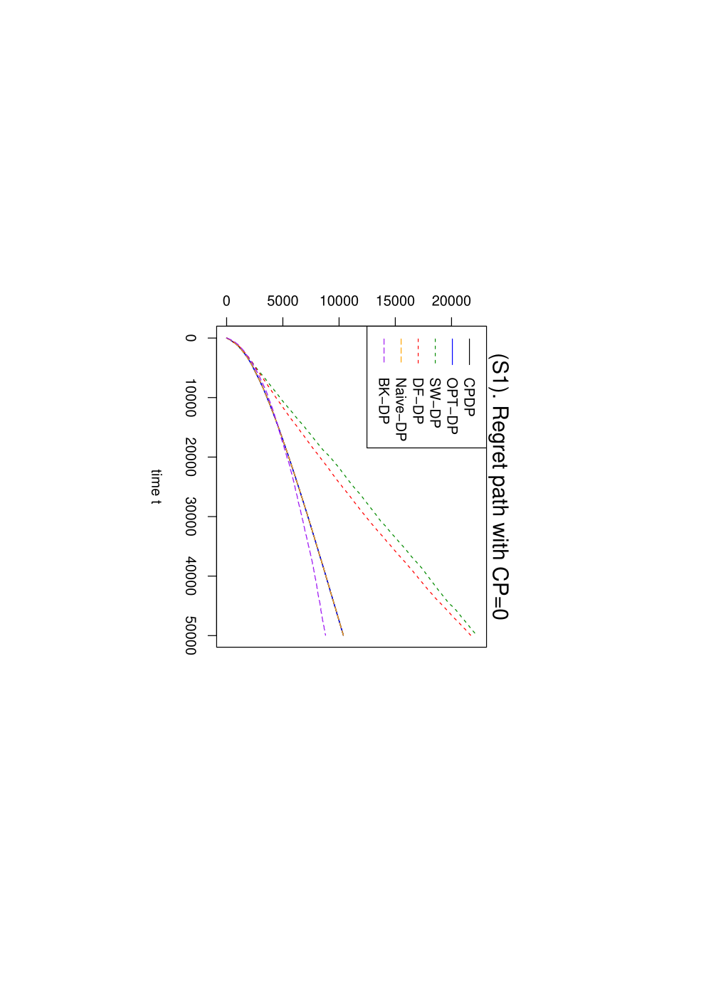
Refer to caption
Refer to caption
Refer to caption
Figure 3: Mean regret path at horizon T=50000T=50000 under (S1) [left] and (S3) [middle, right] with λfix=0.2​log⁡(T​d)\lambda_{\mathrm{fix}}=0.2\sqrt{\log(Td)}. Two plots are provided under (S3) for better visualization. The vertical dotted lines (black and blue) mark the (true and estimated) change-point locations.

5.2.2 Sensitivity Analysis of the Tuning Parameter λ\lambda:

In this section, we further investigate the impact of Lasso tuning parameter λ\lambda on the performance of each algorithm. Figure 4 (left and middle) reports the mean regret R¯T=∑i=1100RT(i)/100\overline{R}_{T}=\sum_{i=1}^{100}R_{T}^{(i)}/100 of each algorithm at different horizon TT under simulation scenarios (S1) and (S3), where λcv\lambda_{\mathrm{cv}} is used in the Lasso penalty. The result under (S2) is similar and thus omitted. Compared with Figure 2, the performance of each algorithm is rather stable. OPT-DP and CPDP are still the overall winners. For illustration, at T=10000T=10000, the minimum, 25%, 50%, 75% and maximum quantiles of {λcv(i)}i=1100\{\lambda_{\mathrm{cv}}^{(i)}\}_{i=1}^{100} are 0.483,0.766,0.848,0.960,1.2650.483,0.766,0.848,0.960,1.265, respectively, while λfix=0.2​log⁡(T​d)=0.724.\lambda_{\mathrm{fix}}=0.2\sqrt{\log(Td)}=0.724.

Figure 4 (right) further reports the mean regret of CPDP under (S3) with λcv\lambda_{\mathrm{cv}} and λfix=cλ​log⁡(T​d)\lambda_{\mathrm{fix}}=c_{\lambda}\sqrt{\log(Td)} at cλ=0.05,0.1,0.2,0.5,1,2.c_{\lambda}=0.05,0.1,0.2,0.5,1,2. As can be seen, the performance of CPDP with λcv\lambda_{\mathrm{cv}} is comparable to the best-performing λfix.\lambda_{\mathrm{fix}}. In addition, CPDP is reasonably robust to the tuning parameter cλc_{\lambda}, except for cλ=0.05c_{\lambda}=0.05. In particular, an overly small cλc_{\lambda} leads to high variance in the Lasso estimation, which in turn leads to false positives in change-point detection. For illustration, at T=10000T=10000, the means of the number of change-points detected at cλ=0.05,0.1,0.2,0.5,1,2c_{\lambda}=0.05,0.1,0.2,0.5,1,2 are 10.79, 5.32, 3.01, 3.00, 3.00, 3.00, respectively.

Refer to caption
Refer to caption
Refer to caption
Figure 4: [Left and middle]: Mean regret vs. TT under (S1) and (S3) with λcv\lambda_{\mathrm{cv}}. [Right]: Mean regret vs. TT by CPDP under (S3) with λcv\lambda_{\mathrm{cv}} and λfix=cλ​log⁡(T​d)\lambda_{\mathrm{fix}}=c_{\lambda}\sqrt{\log(Td)} at cλ=0.05,0.1,0.2,0.5,1,2c_{\lambda}=0.05,0.1,0.2,0.5,1,2.

5.2.3 Performance with Varying Change Sizes:

In this section, we investigate the impact of change size on the performance of each algorithm. In particular, we modify the simulation scenarios (S2) and (S3) in Section 5.2.1 with θ(1)=(0,1,1,2,2,𝟎44⊤,−0.25)⊤\theta^{(1)}=(0,1,1,2,2,\mathbf{0}_{44}^{\top},-0.25)^{\top} unchanged but replace θ(2)\theta^{(2)} with θ(2)∗=(0,1.5,1.5,2,2,𝟎44⊤,−0.5)⊤\theta^{(2)*}=(0,1.5,1.5,2,2,\mathbf{0}_{44}^{\top},-0.5)^{\top}. Denote the new scenarios as (S2)∗ and (S3)∗.

Compared to θ(2)\theta^{(2)}, θ(2)∗\theta^{(2)*} has the same price sensitivity 0.50.5 but much higher attractiveness 𝔼⁡(αt⊤​zt)=3.5\mathbb{E}(\alpha_{t}^{\top}z_{t})=3.5 instead of 2. Thus, when switching from θ(1)\theta^{(1)} to θ(2)∗\theta^{(2)*}, though price sensitivity is higher, due to the increased attractiveness, the optimal price may not change as much, which intuitively implies less value for change-point detection. Indeed, for {pt}∼i.i.d.uniform​[p~l,p~u]\{p_{t}\}\stackrel{{\scriptstyle\mbox{i.i.d.}}}{{\sim}}\text{uniform}[\widetilde{p}_{l},\widetilde{p}_{u}], the KL divergence between θ(1)\theta^{(1)} and θ(2)\theta^{(2)}, θ(2)∗\theta^{(2)*} are

KL(θ(1),θ(2))=𝔼θ(1)(logPθ(1)​(yt|zt,pt)Pθ(2)​(yt|zt,pt))=0.814, and KL(θ(1),θ(2)∗)=0.282.\displaystyle\text{KL}(\theta^{(1)},\theta^{(2)})=\mathbb{E}_{\theta^{(1)}}\left(\log\frac{P_{\theta^{(1)}}(y_{t}|z_{t},p_{t})}{P_{\theta^{(2)}}(y_{t}|z_{t},p_{t})}\right)=0.814,\text{ and }\text{KL}(\theta^{(1)},\theta^{(2)*})=0.282.

Thus, compared to θ(2)\theta^{(2)}, it is more difficult (and also less valuable) to differentiate θ(1)\theta^{(1)} and θ(2)∗\theta^{(2)*}.

Figure 5 (left and middle) reports the mean regret R¯T=∑i=1100RT(i)/100\overline{R}_{T}=\sum_{i=1}^{100}R_{T}^{(i)}/100 of each algorithm at different horizon TT under simulation scenarios (S2)∗ and (S3)∗. Compared to Figure 2, the notable difference is that the performance gaps between CPDP and competitors are smaller. For example, at T=50000T=50000, for (S3), the ratio of regret by SW-DP, DF-DP, and Naive-DP with respect to CPDP are 1.32, 1.36 and 2.85, while for (S3)∗, the corresponding ratios are 1.12, 1.09 and 1.83. In addition, due to larger detection delay, the gaps between CPDP and OPT-DP are wider.

Refer to caption
Refer to caption
Refer to caption
Figure 5: [Left and middle]: Mean regret vs. TT under (S2)∗ and (S3)∗ with λfix=0.2​log⁡(T​d)\lambda_{\mathrm{fix}}=0.2\sqrt{\log(Td)}. [Right]: Mean regret path at horizon T=50000T=50000 under (S3)∗ with λfix=0.2​log⁡(T​d)\lambda_{\mathrm{fix}}=0.2\sqrt{\log(Td)}. The vertical dotted lines (black and blue) mark the (true and estimated) change-point locations.

In particular, Table 1 reports the average numbers of detected change-points across 100 experiments by CPDP under (S3) and (S3)∗ for different horizon TT. As can be seen, CPDP successfully detects all change-points for (S3) but experiences some under-detection for (S3)∗ when TT is small. Denote τ^1−τ1\widehat{\tau}_{1}-\tau_{1} as the detection delay for the first change-point τ1=T/4\tau_{1}=T/4. Table 1 further reports the ratio between average detection delay by CPDP under (S3)∗ and (S3). Compared to (S3), CPDP has around three times longer detection delay for τ1\tau_{1} under (S3)∗. This can be further seen by comparing Figure 3 (middle) and Figure 5 (right), which give the mean regret path of CPDP at horizon T=50000T=50000 under (S3) and (S3)∗, respectively.

Table 1: Average number of detected change-points under (S3) and (S3)∗. “Ratio” gives the ratio between average detection delay for the first change-point (τ1\tau_{1}) under (S3)∗ and (S3).
TT 5000 10000 20000 30000 40000 50000 60000 70000 80000 90000 100000
(S3) 3.00 3.00 3.00 3.00 3.01 3.00 3.00 3.00 3.00 3.00 3.00
(S3)∗ 2.58 2.99 3.00 3.00 3.00 3.00 3.00 3.00 3.00 3.00 3.00
Ratio 2.79 3.02 2.95 3.64 3.36 2.70 3.28 3.00 3.72 2.67 3.55

In Section G.2, we further modify scenarios (S1), (S2) and (S3) by replacing θ(1)\theta^{(1)} with θ(3)=θ(1)/2\theta^{(3)}=\theta^{(1)}/2 and replacing θ(2)\theta^{(2)} with θ(4)=θ(2)/2\theta^{(4)}=\theta^{(2)}/2, such that the change size is halved. The observation is the same: CPDP still provides the best overall performance albeit at a smaller scale of improvement.

5.2.4 Scaling with respect to the Numbers of Change-Points ΥT\Upsilon_{T}:

In this section, we investigate the performance of CPDP with respect to the number of change-points ΥT.\Upsilon_{T}. Denote 𝕀=10000\mathbb{I}=10000. We design (S4) such that

(S4):θt={θ(1),t∈[k𝕀+1,(k+1)𝕀],k=0,2,4,…,k≤ΥT;θ(2),t∈[k𝕀+1,(k+1)𝕀],k=1,3,5,…,k≤ΥT.\displaystyle\text{(S4)}:\theta_{t}=\begin{cases}\theta^{(1)},&t\in[k\mathbb{I}+1,(k+1)\mathbb{I}],k=0,2,4,\ldots,~k\leq\Upsilon_{T};\\ \theta^{(2)},&t\in[k\mathbb{I}+1,(k+1)\mathbb{I}],k=1,3,5,\ldots,~k\leq\Upsilon_{T}.\\ \end{cases}\quad

By design, T=(ΥT+1)​𝕀T=(\Upsilon_{T}+1)\mathbb{I} and the process alternates between θ(1)\theta^{(1)} and θ(2)\theta^{(2)} with ΥT\Upsilon_{T} number of change-points. We set λfix=0.2​log⁡(T​d)\lambda_{\mathrm{fix}}=0.2\sqrt{\log(Td)}.

Figure 6 (left) reports the mean regret R¯T\overline{R}_{T} with respect to ΥT​T\Upsilon_{T}T of each algorithm for ΥT=2,4,8,10,15,20\Upsilon_{T}=2,4,8,10,15,20, where the regret by CPDP resembles the shape of a square-root function. A linear regression between log⁡(R¯T)\log(\overline{R}_{T}) and log⁡(ΥT​T)\log(\Upsilon_{T}T) for CPDP gives a slope of 0.5016, providing numerical evidence that the regret by CPDP scales at the rate of ΥT​T\sqrt{\Upsilon_{T}T} as in 2. Figure 6 (right) plots the detection delay of τk\tau_{k} (averaged across 100 experiments) for k=1,…,ΥTk=1,\ldots,\Upsilon_{T} when ΥT=20\Upsilon_{T}=20. It is clear that the detection delay decreases with kk, indicating the effectiveness of the accelerated exploration mechanism in Algorithm 1. Note that we separate τk\tau_{k} by even and odd kk as the difficulty of detecting a switch from θ(1)\theta^{(1)} to θ(2)\theta^{(2)} is different than a switch from θ(2)\theta^{(2)} to θ(1)\theta^{(1)}.

Refer to caption
Refer to caption
Figure 6: [Left]: Mean regret vs. ΥT​T\Upsilon_{T}T for ΥT=2,4,8,10,15,20\Upsilon_{T}=2,4,8,10,15,20. [Right]: Average detection delay of τk\tau_{k} for k=1,2,…,ΥTk=1,2,\ldots,\Upsilon_{T} at ΥT=20\Upsilon_{T}=20.

5.3 Real Data Applications

In this section, we explore practical utility of CPDP on a real-world auto loan dataset provided by the Center for Pricing and Revenue Management at Columbia University. This dataset was first studied by Phillips et al. 2015 and further used by Bastani et al. 2022, Ban and Keskin 2021, Luo et al. 2021 to evaluate various dynamic pricing algorithms under different problem settings.

The dataset records all auto loan applications received by a major online lender in the U.S. from July 2002 to November 2004. We use the first 50000 loan applications for the case study. For each application, we observe information about the loan (e.g., term and amount), the prospective consumer (e.g., FICO score), and the economic environment (e.g., prime rate). We refer to Section G.3 for detailed description of the dataset. We also observe the monthly payment required for the approved loan, which can be viewed as the pricing decision by the company, and whether the offer was accepted – a binary purchasing decision by a consumer.

We follow the feature selection result in Luo et al. 2021 and Bastani et al. 2022, and consider the loan amount approved, term, prime rate, the competitor’s rate and FICO score as covariates with non-zero coefficients, and treat the rest nine features in the dataset as zero/null covariates. The price pp of a loan is computed as the net present value of future payment minus the loan amount, i.e., p=Monthly Payment×∑i=1Term(1+Rate)−i−Loan Amount.p=\text{Monthly Payment}\times\sum_{i=1}^{\text{Term}}(1+\text{Rate})^{-i}-\text{Loan Amount}. We set Rate as 0.12%0.12\%, an average of the monthly London interbank offered rate for the studied time period. Denote the ttth consumer decision as yty_{t}, non-zero covariates as zt∗z_{t}^{*}, all covariates as ztz_{t}, and loan price as pt.p_{t}. For convenience, we use one thousand dollars as the basic unit for loan price and loan amount.

Note that it is impossible to obtain consumers’ real online responses to any dynamic pricing strategy unless it was used in the system when the data were collected. Thus, following the literature, we first estimate the demand model based on the entire 50000 observations and use it as the ground truth to generate consumer responses. Specifically, we run a standard model selection based offline change-point detection algorithm (Davis et al. 2006, Bai and Perron 2003, e.g.,) on {(yt,zt∗,pt)}t=150000\{(y_{t},z_{t}^{*},p_{t})\}_{t=1}^{50000}, which returns three change-points at t=12916,24986,37054.t=12916,24986,37054. We refer to Section G.3 for a more detailed description of the offline change-point detection algorithm. Table 2 gives the estimated logistic regression based on each stationary segment, where notable changes (such as sensitivity to price and competitor’s rate) can be observed. As discussed in the Section 1, this confirms the informal change-point analysis in Besbes and Zeevi 2011.

Table 2: Estimated logistic regression on each stationary segments. Coefficients for FICO and Term are in the scale of ×10−3\times 10^{-3} and ×10−2\times 10^{-2}.
Segment Intercept Price FICO Competitor Rate Amount Prime Rate Term
[1,12916][1,12916] -7.63 -0.42 3.20 1.83 -0.11 -2.00 1.47
[12917,24986][12917,24986] -12.29 -0.60 0.35 2.69 -0.07 -0.63 1.43
[24986,37054][24986,37054] -12.81 -1.27 -7.24 4.77 -0.02 -1.92 2.89
[37054,50000][37054,50000] -7.66 -0.88 -2.37 2.77 -0.09 -1.02 0.57

We run all algorithms based on the ground truth model in Table 2. For the Lasso tuning parameter λ\lambda, we use both λfix=0.02​log⁡(T​d)\lambda_{\mathrm{fix}}=0.02\sqrt{\log(Td)} and λcv\lambda_{\mathrm{cv}}. We set the price experiment set 𝒫~\widetilde{\mathcal{P}} as [p~l,p~u]=[0.2,6][\widetilde{p}_{l},\widetilde{p}_{u}]=[0.2,6] and set the price bound as [pl,pu]=[0,14].[p_{l},p_{u}]=[0,14]. For reference, the min, max, median and mean prices given by the company are 0.2,13.5,2.60.2,13.5,2.6 and 2.92.9 in the studied period. We remark that the result is robust to the choice of [p~l,p~u][\widetilde{p}_{l},\widetilde{p}_{u}]. For each algorithm, we conduct 100 experiments and record regret {RT(i)}i=1100\{R_{T}^{(i)}\}_{i=1}^{100}. Note that for all experiments, we keep the sample path of the covariates {zt}t=150000\{z_{t}\}_{t=1}^{50000} fixed as that in the dataset.

Figure 7 (left and middle) give the mean regret path of each algorithm based on λfix\lambda_{\mathrm{fix}} and λcv\lambda_{\mathrm{cv}}, where the results are almost identical, indicating the robustness of the finding. For reference, the minimum, 25%, 50%, 75% and maximum quantiles of {λcv(i)}i=1100\{\lambda_{\mathrm{cv}}^{(i)}\}_{i=1}^{100} are 0.0119,0.106,0.164,0.2210.0119,0.106,0.164,0.221 and 0.5250.525, respectively, while λfix=0.02​log⁡(T​d)=0.0735.\lambda_{\mathrm{fix}}=0.02\sqrt{\log(Td)}=0.0735.

Figure 7 (right) further gives the boxplot of {RT(i)}i=1100\{R_{T}^{(i)}\}_{i=1}^{100} for each algorithm, where CPDP and OPT-DP are the clear overall winners. In particular, the mean regret (in thousands) by CPDP, OPT-DP, SW-DP, DF-DP, Naive-DP and BK-DP are 1953, 1795, 2247, 2593, 3315 and 4392. For reference, the regret incurred by the company pricing policy is 7206. Thus, compared to Naive-DP and BK-DP, CPDP reduces revenue loss by 1.3∼\sim2.3 million dollars, indicating the importance of handling non-stationarity in dynamic pricing. The expected revenue by optimal pricing is 25078. It is easy to see that CPDP lifts revenue by 29%, 11.4% and 6.1% when compared with the company policy, BK-DP and Naive-DP.

Refer to caption
Refer to caption
Refer to caption
Figure 7: [Left and middle]: Mean regret path with λfix=0.02​log⁡(T​d)\lambda_{\mathrm{fix}}=0.02\sqrt{\log(Td)} and λcv\lambda_{\mathrm{cv}}. The vertical dotted lines (black and blue) mark the (true and estimated) change-point locations. [Right]: Boxplot of regret based on 100 experiments with λfix=0.02​log⁡(T​d)\lambda_{\mathrm{fix}}=0.02\sqrt{\log(Td)}. Red dots indicate mean.

6 Conclusion and Discussion

In this paper, we study a dynamic pricing problem under non-stationarity, where the demand model is a GLM with high-dimensional contextual information. We propose the CPDP algorithm, which achieves a near-optimal regret of order O⁡(s​ΥT​T​log⁡(T​d)).O(s\sqrt{\Upsilon_{T}T}\log(Td)). To our best knowledge, CPDP is the first algorithm in the dynamic pricing literature that handles non-stationary demand models with covariates. Compared to existing works, CPDP does not require the knowledge of a lower bound on the change size, and its regret scales optimally with the number of change-points ΥT\Upsilon_{T}, owing to a novel accelerated exploration mechanism. As an important byproduct, we develop an online change-point detection algorithm for high-dimensional GLMs, which on its own, is optimal and novel in the online change-point detection literature.

In this paper, we assume full access to consumer-level transaction data, which may include sensitive information such as consumer demographics. With the increasing awareness of privacy, it would be interesting and timely to develop a dynamic pricing policy that can handle non-stationarity subject to privacy constraints. We leave this for future research.

References

  • Agresti (2015) Agresti A (2015) Foundations of Linear and Generalized Linear Models (John Wiley & Sons).
  • Araman and Caldentey (2009) Araman VF, Caldentey R (2009) Dynamic pricing for nonperishable products with demand learning. Operations Research 57(5):1169–1188.
  • Auer et al. (2002) Auer P, Cesa-Bianchi N, Freund Y, Schapire RE (2002) The nonstochastic multiarmed bandit problem. SIAM Journal on Computing 32(1):48–77.
  • Bai and Perron (2003) Bai J, Perron P (2003) Computation and analysis of multiple structural change models. Journal of Applied Econometrics 18(1):1–22.
  • Ban and Keskin (2021) Ban GY, Keskin NB (2021) Personalized dynamic pricing with machine learning: High-dimensional features and heterogeneous elasticity. Management Science 67(9):5549–5568.
  • Bastani et al. (2022) Bastani H, Simchi-Levi D, Zhu R (2022) Meta dynamic pricing: Transfer learning across experiments. Management Science 68(3):1865–1881.
  • Bauer et al. (2020) Bauer H, Burkacky O, Kenevan P, Mahindroo A, Patel M (2020) How the semiconductor industry can emerge stronger after the COVID-19 crisis. Technical report, McKinsey.
  • Berge (1957) Berge C (1957) Two theorems in graph theory. Proceedings of the National Academy of Sciences 43(9):842–844.
  • Besbes et al. (2014) Besbes O, Gur Y, Zeevi A (2014) Stochastic multi-armed-bandit problem with non-stationary rewards. Advances in Neural Information Processing Systems 27.
  • Besbes and Zeevi (2009) Besbes O, Zeevi A (2009) Dynamic pricing without knowing the demand function: Risk bounds and near-optimal algorithms. Operations Research 57(6):1407–1420.
  • Besbes and Zeevi (2011) Besbes O, Zeevi A (2011) On the minimax complexity of pricing in a changing environment. Operations Research 59(1):66–79.
  • Besson et al. (2022) Besson L, Kaufmann E, Maillard OA, Seznec J (2022) Efficient change-point detection for tackling piecewise-stationary bandits. Journal of Machine Learning Research .
  • Broder and Rusmevichientong (2012) Broder J, Rusmevichientong P (2012) Dynamic pricing under a general parametric choice model. Operations Research 60(4):965–980.
  • Brodsky and Darkhovsky (1993) Brodsky E, Darkhovsky BS (1993) Nonparametric Methods in Change Point Problems (Springer Science & Business Media).
  • Bühlmann and Van De Geer (2011) Bühlmann P, Van De Geer S (2011) Statistics for High-Dimensional Data: Methods, Theory and Applications (Springer Science & Business Media).
  • Cao et al. (2019) Cao Y, Zheng W, Kveton B, Xie Y (2019) Nearly optimal adaptive procedure for piecewise-stationary bandit: a change-point detection approach. AISTATS, Okinawa, Japan .
  • Chen (2019) Chen H (2019) Sequential change-point detection based on nearest neighbors. Annals of Statistics 47(3):1381–1407.
  • Chen and Gupta (2012) Chen J, Gupta AK (2012) Parametric Statistical Change Point Analysis (Springer).
  • Chen and Gallego (2019) Chen N, Gallego G (2019) Welfare analysis of dynamic pricing. Management Science 65(1):139–151.
  • Chen and Gallego (2021) Chen N, Gallego G (2021) Nonparametric pricing analytics with customer covariates. Operations Research 69(3):974–984.
  • Chen et al. (2022) Chen X, Miao S, Wang Y (2022) Differential privacy in personalized pricing with nonparametric demand models. Operations Research .
  • Chen et al. (2023) Chen Y, Wen Z, Xie Y (2023) Dynamic pricing in an evolving and unknown marketplace. Management Science, to appear .
  • Cheung et al. (2017) Cheung WC, Simchi-Levi D, Wang H (2017) Dynamic pricing and demand learning with limited price experimentation. Operations Research 65(6):1722–1731.
  • Cheung et al. (2019) Cheung WC, Simchi-Levi D, Zhu R (2019) Learning to optimize under non-stationarity. The 22nd International Conference on Artificial Intelligence and Statistics, 1079–1087 (PMLR).
  • Cheung et al. (2022) Cheung WC, Simchi-Levi D, Zhu R (2022) Hedging the drift: Learning to optimize under nonstationarity. Management Science 68(3):1696–1713.
  • Davis et al. (2006) Davis RA, Lee TCM, Rodriguez-Yam GA (2006) Structural break estimation for nonstationary time series models. Journal of the American Statistical Association 101(473):223–239.
  • den Boer and Zwart (2015) den Boer AV, Zwart B (2015) Dynamic pricing and learning with finite inventories. Operations Research 63(4):965–978.
  • Dubey et al. (2021) Dubey P, Xu H, Yu Y (2021) Online network change point detection with missing values. arXiv preprint arXiv:2110.06450 .
  • Farias and Van Roy (2010) Farias VF, Van Roy B (2010) Dynamic pricing with a prior on market response. Operations Research 58(1):16–29.
  • Garivier and Moulines (2011) Garivier A, Moulines E (2011) On upper-confidence bound policies for switching bandit problems. International Conference on Algorithmic Learning Theory, 174–188 (Springer).
  • Harrison et al. (2012) Harrison JM, Keskin NB, Zeevi A (2012) Bayesian dynamic pricing policies: Learning and earning under a binary prior distribution. Management Science 58(3):570–586.
  • He et al. (2018) He X, Xie Y, Wu SM, Lin FC (2018) Sequential graph scanning statistic for change-point detection. 2018 52nd Asilomar Conference on Signals, Systems, and Computers, 1317–1321 (IEEE).
  • Javanmard and Nazerzadeh (2019) Javanmard A, Nazerzadeh H (2019) Dynamic pricing in high-dimensions. Journal of Machine Learning Research 20(1):315–363.
  • Jia et al. (2022) Jia H, Shi C, Shen S (2022) Online learning and pricing for service systems with reusable resources. Operations Research, in press .
  • Kaul et al. (2019) Kaul A, Jandhyala VK, Fotopoulos SB (2019) An efficient two step algorithm for high dimensional change point regression models without grid search. Journal of Machine Learning Research 20:111–1.
  • Keshavarz et al. (2020) Keshavarz H, Michailidis G, Atchadé Y (2020) Sequential change-point detection in high-dimensional gaussian graphical models. Journal of Machine Learning Research 21(1):3125–3181.
  • Keskin et al. (2022) Keskin NB, Li Y, Song JS (2022) Data-driven dynamic pricing and ordering with perishable inventory in a changing environment. Management Science 68(3):1938–1958.
  • Keskin and Zeevi (2014) Keskin NB, Zeevi A (2014) Dynamic pricing with an unknown demand model: Asymptotically optimal semi-myopic policies. Operations Research 62(5):1142–1167.
  • Keskin and Zeevi (2017) Keskin NB, Zeevi A (2017) Chasing demand: Learning and earning in a changing environment. Mathematics of Operations Research 42(2):277–307.
  • Kocsis and Szepesvári (2006) Kocsis L, Szepesvári C (2006) Bandit based monte-carlo planning. Machine Learning: ECML 2006: 17th European Conference on Machine Learning Berlin, Germany, September 18-22, 2006 Proceedings 17, 282–293 (Springer).
  • Lai (1995) Lai TL (1995) Sequential changepoint detection in quality control and dynamical systems. Journal of the Royal Statistical Society: Series B: Statistical Methodology 57(4):613–644.
  • Lai (1998) Lai TL (1998) Information bounds and quick detection of parameter changes in stochastic systems. IEEE Transactions on Information Theory 44(7):2917–2929.
  • Lai and Xing (2010) Lai TL, Xing H (2010) Sequential change-point detection when the pre-and post-change parameters are unknown. Sequential Analysis 29(2):162–175.
  • Lee et al. (2016) Lee S, Seo MH, Shin Y (2016) The lasso for high dimensional regression with a possible change point. Journal of the Royal Statistical Society: Series B: Statistical Methodology 78(1):193–210.
  • Liu et al. (2018) Liu F, Lee J, Shroff N (2018) A change-detection based framework for piecewise-stationary multi-armed bandit problem. Proceedings of the AAAI Conference on Artificial Intelligence 32(1).
  • Luo et al. (2021) Luo Y, Sun WW, Liu Y (2021) Distribution-free contextual dynamic pricing. arXiv preprint arXiv:2109.07340 .
  • Maillard (2019) Maillard OA (2019) Sequential change-point detection: Laplace concentration of scan statistics and non-asymptotic delay bounds. Algorithmic Learning Theory, 610–632 (PMLR).
  • Nambiar et al. (2019) Nambiar M, Simchi-Levi D, Wang H (2019) Dynamic learning and pricing with model misspecification. Management Science 65(11):4980–5000.
  • Negahban et al. (2012) Negahban SN, Ravikumar P, Wainwright MJ, Yu B (2012) A unified framework for high-dimensional analysis of mm-estimators with decomposable regularizers. Statistical Science 27(4):538–557.
  • Phillips et al. (2015) Phillips R, Şimşek AS, Van Ryzin G (2015) The effectiveness of field price discretion: Empirical evidence from auto lending. Management Science 61(8):1741–1759.
  • Pollard (1990) Pollard D (1990) Empirical processes: Theory and applications. NSF-CBMS Regional Conference Series in Probability and Statistics, 2. Institute of Mathematical Statistics, Hayward, CA; American Statistical Association, Alexandria, VA .
  • Raskutti et al. (2010) Raskutti G, Wainwright MJ, Yu B (2010) Restricted eigenvalue properties for correlated gaussian designs. Journal of Machine Learning Research 11:2241–2259.
  • Rinaldo et al. (2021) Rinaldo A, Wang D, Wen Q, Willett R, Yu Y (2021) Localizing changes in high-dimensional regression models. International Conference on Artificial Intelligence and Statistics, 2089–2097 (PMLR).
  • Safikhani and Shojaie (2022) Safikhani A, Shojaie A (2022) Joint structural break detection and parameter estimation in high-dimensional nonstationary var models. Journal of the American Statistical Association 117(537):251–264.
  • Seznec et al. (2020) Seznec J, Menard P, Lazaric A, Valko M (2020) A single algorithm for both restless and rested rotting bandits. International Conference on Artificial Intelligence and Statistics, 3784–3794 (PMLR).
  • Siegmund (1985) Siegmund D (1985) Sequential analysis: tests and confidence intervals (Springer Science & Business Media).
  • Tarlton (2020) Tarlton A (2020) 24 things that have been selling out online during the coronavirus pandemic. USA Today .
  • Tartakovsky et al. (2014) Tartakovsky A, Nikiforov I, Basseville M (2014) Sequential Analysis: Hypothesis Testing and Change point Detection (CRC Press).
  • Tibshirani (1996) Tibshirani R (1996) Regression shrinkage and selection via the lasso. Journal of the Royal Statistical Society: Series B: Statistical Methodology 58(1):267–288.
  • Tsybakov (2009) Tsybakov A (2009) Introduction to Nonparametric Estimation (Springer, New York).
  • Wainwright (2019) Wainwright MJ (2019) High-Dimensional Statistics: A Non-Asymptotic Viewpoint (Cambridge University Press).
  • Wang et al. (2020) Wang D, Yu Y, Willett R (2020) Detecting abrupt changes in high-dimensional self-exciting poisson processes. arXiv preprint arXiv:2006.03572 .
  • Wang et al. (2021a) Wang D, Zhao Z, Lin KZ, Willett R (2021a) Statistically and computationally efficient change point localization in regression settings. Journal of Machine Learning Research 22(1):11255–11300.
  • Wang et al. (2021b) Wang Y, Chen B, Simchi-Levi D (2021b) Multimodal dynamic pricing. Management Science 67(10):6136–6152.
  • Whitten (2020) Whitten S (2020) What people are buying as they heed coronavirus stay-at-home orders. CNBC .
  • Yu (2020) Yu Y (2020) A review on minimax rates in change point detection and localisation. arXiv preprint arXiv:2011.01857 .
  • Yu et al. (2020) Yu Y, Padilla OHM, Wang D, Rinaldo A (2020) A note on online change point detection. arXiv preprint arXiv:2006.03283 .

Online Appendix

High-Dimensional Dynamic Pricing under Non-Stationarity: Learning and Earning with Change-Point Detection

The Appendix is organized as follows. Section A derives useful properties of the revenue function, which are used throughout the proof. Section B and Section C provide estimation error bounds of the Lasso estimator for a single GLM and a mixture of two GLMs, respectively. Section D proves the theoretical guarantee of the change-point detector given in 1. Section E proves the regret upper bound of CPDP in 1 and 1. Section F proves the regret lower bound in 2. Section G gives additional numerical results.

The estimation error bounds derived in Section B are used in Section D for establishing theoretical guarantees (i.e., false alarm, detection delay) of the online change-point detection algorithm. The estimation error bounds in Section B, Section C and the theoretical guarantees of the online change-point detection algorithm in Section D are further used in Section E for establishing the regret upper bound of the CPDP algorithm.

A Properties of the Revenue Function

This section derives two useful properties of the revenue function. The first property shows φ\varphi is Lipschitz as promised in (4), and the second property suggests the revenue loss (instant regret) can be bounded above by the squared price differences.

A.1 Lipschitz property of φ\varphi

Lemma EC.1

Under 1, there exists a continuous function φ⁡(u,v){\varphi}(u,v) such that

pt∗=φ⁡(αt⊤​zt,βt),p_{t}^{*}={\varphi}(\alpha_{t}^{\top}z_{t},\beta_{t}),

for all t∈{1,2,⋯,T}.t\in\{1,2,\cdots,T\}.

By Lemma EC.1, pt∗p_{t}^{*} is a continuous function of αt⊤​zt\alpha_{t}^{\top}z_{t} and βt\beta_{t}. Under Assumption 1, we further have |zt⊤​αt|≤‖zt‖∞​‖αt‖1≤Cb​Cθ|z_{t}^{\top}\alpha_{t}|\leq\|z_{t}\|_{\infty}\|\alpha_{t}\|_{1}\leq C_{b}C_{\theta} and |βt|≤Cθ|\beta_{t}|\leq C_{\theta}. Together with Lemma EC.1, this implies the Lipschitz continuity in (4), as a continuous function is Lipschitz continuous on a compact set. Throughout the Appendix, with a slight abuse of notation, we further denote pt∗=φ⁡(αt⊤​zt,βt)=φ⁡(θt,zt)p_{t}^{*}={\varphi}(\alpha_{t}^{\top}z_{t},\beta_{t})={\varphi}(\theta_{t},z_{t}).

Proof of Lemma EC.1: Recall that r(pt,θt,zt)=pt𝔼[yt|pt,zt]=ptψ′(zt⊤αt+βtpt).r(p_{t},\theta_{t},z_{t})=p_{t}\mathbb{E}[y_{t}|p_{t},z_{t}]=p_{t}\psi^{\prime}(z_{t}^{\top}\alpha_{t}+\beta_{t}p_{t}). By definition,

pt∗=\argmaxp∈[pl,pu]​p⋅ψ′​(αt⊤​zt+βt​p).\displaystyle p_{t}^{*}=\argmax_{p\in[p_{l},p_{u}]}p\cdot\psi^{\prime}(\alpha_{t}^{\top}z_{t}+\beta_{t}p).

Thus, pt∗p_{t}^{*} depends on θt\theta_{t} and ztz_{t} via αt⊤​zt\alpha_{t}^{\top}z_{t} and βt\beta_{t}. By Assumption 1(iv), for any θt\theta_{t} and ztz_{t}, pt∗p_{t}^{*} is unique. Thus, pt∗p_{t}^{*} is in fact a function of αt⊤​zt\alpha_{t}^{\top}z_{t} and βt\beta_{t} and can be written as pt∗=φ⁡(αt⊤​zt,βt)p_{t}^{*}={\varphi}(\alpha_{t}^{\top}z_{t},\beta_{t}). We next prove that φ⁡(u,v){\varphi}(u,v) is continuous.

To apply Berge’s Maximum Theorem (Berge 1957), we first define Γ⁡(u,v)=[pl,pu]\Gamma(u,v)=[p_{l},p_{u}] for any u,vu,v. Note that Γ⁡(u,v)\Gamma(u,v) is a set-valued function and is continuous at any (u,v)(u,v). By the definition of φ⁡(u,v)\varphi(u,v), we have that

φ⁡(u,v)=\argmaxp∈[pl,pu]​p⋅ψ′​(u+v​p)=\argmaxp∈Γ⁡(u,v)​p⋅ψ′​(u+v​p).\displaystyle\varphi(u,v)=\argmax_{p\in[p_{l},p_{u}]}p\cdot\psi^{\prime}(u+vp)=\argmax_{p\in\Gamma(u,v)}p\cdot\psi^{\prime}(u+vp).

By 1(iii), p⋅ψ′​(u+v​p)p\cdot\psi^{\prime}(u+vp) is a continuous function of (p,u,v)(p,u,v). Together with the fact that Γ⁡(u,v)\Gamma(u,v) is continuous at any (u,v)(u,v), by Berge’s Maximum Theorem, we have that φ⁡(u,v)\varphi(u,v) (as a set-valued function) is upper hemicontinuous. However, by 1(iv), φ⁡(u,v)\varphi(u,v) is indeed a function. Thus, by the definition of upper hemicontinuity, we have that φ⁡(u,v)\varphi(u,v) is continuous. ∎

A.2 Bound instant regret by square of price difference

As another consequence of Assumption 1, given θt\theta_{t} and ztz_{t}, for any fixed price ptp_{t}, we have

r⁡(pt,θt,zt)=r⁡(pt∗,θt,zt)+∂r⁡(pt∗,θt,xt)∂p⏟=0​(pt−pt∗)+12​∂2r⁡(p~,θt,zt)∂p2​(pt−pt∗)2,\displaystyle r(p_{t},\theta_{t},z_{t})=r(p_{t}^{*},\theta_{t},z_{t})+\underbrace{\frac{\partial r(p_{t}^{*},\theta_{t},x_{t})}{\partial p}}_{=0}(p_{t}-p_{t}^{*})+\frac{1}{2}\frac{\partial^{2}r(\widetilde{p},\theta_{t},z_{t})}{\partial p^{2}}(p_{t}-p_{t}^{*})^{2},

for some p~\widetilde{p} lies between ptp_{t} and pt∗p_{t}^{*} with pt∗=φ⁡(θt,zt)p_{t}^{*}={\varphi}(\theta_{t},z_{t}). This implies the instant regret is quadratic in terms of the price difference between ptp_{t} and optimal price pt∗p_{t}^{*}.

Furthermore, 1 also implies that

sup‖z‖∞≤Cb,p∈[pl,pu],‖θ‖1≤Cθ|12​∂2r⁡(p,θ,z)∂p2|=Cr<∞.\sup_{\|z\|_{\infty}\leq C_{b},p\in[p_{l},p_{u}],\|\theta\|_{1}\leq C_{\theta}}\left|\frac{1}{2}\frac{\partial^{2}r(p,\theta,z)}{\partial p^{2}}\right|=C_{r}<\infty. (EC.1)

Therefore,

r⁡(pt∗,θt,zt)−r⁡(pt,θt,zt)≤Cr​(φ⁡(θt,zt)−pt)2.\displaystyle r(p_{t}^{*},\theta_{t},z_{t})-r(p_{t},\theta_{t},z_{t})\leq C_{r}({\varphi}(\theta_{t},z_{t})-p_{t})^{2}. (EC.2)

B GLM Estimation under Stationarity

This section provides results of the Lasso estimator for a single GLM. In particular, Lemma EC.2 provides a deviation bound for the first order derivatives of the log-likelihood function and Lemma EC.3 derives the restricted strong convexity. Based on Lemma EC.2 and Lemma EC.3, the estimation error bounds of the Lasso estimator is established in Lemma EC.4.

Recall the parameter space Θ={θ∈ℝd:‖θ‖1≤Cθ}\Theta=\{\theta\in\mathbb{R}^{d}:\|\theta\|_{1}\leq C_{\theta}\} for some Cθ>0.C_{\theta}>0. Without loss of generality, we assume Cθ≥1C_{\theta}\geq 1, and pu≤Cbp_{u}\leq C_{b}. Note that ‖θ‖1≤Cθ\|\theta\|_{1}\leq C_{\theta} implies ‖θ‖2≤Cθ\|\theta\|_{2}\leq C_{\theta} and ⟨xt,θ⟩≤‖xt‖∞​‖θ‖1≤Cb​Cθ\langle x_{t},\theta\rangle\leq\|x_{t}\|_{\infty}\|\theta\|_{1}\leq C_{b}C_{\theta}, where xt=(zt⊤,pt)⊤x_{t}=(z_{t}^{\top},p_{t})^{\top}. We denote ψu′′=sup|x|≤(Cθ+1)​Cbψ′′​(x)\psi^{\prime\prime}_{u}=\sup_{|x|\leq(C_{\theta}+1)C_{b}}\psi^{\prime\prime}(x), and ψl′′=inf|x|≤Cb​Cθψ′′​(x)\psi^{\prime\prime}_{l}=\inf_{|x|\leq C_{b}C_{\theta}}\psi^{\prime\prime}(x) such that 0<ψl′′≤ψu′′<∞0<\psi^{\prime\prime}_{l}\leq\psi^{\prime\prime}_{u}<\infty. For any I⊂{1,2,…,T}I\subset\{1,2,\ldots,T\}, define ∇L​(θ,I)=∑t∈I{ψ′​(xt⊤​θ)−yt}​xt\nabla L(\theta,I)=\sum_{t\in I}\{\psi^{\prime}(x^{\top}_{t}\theta)-y_{t}\}x_{t} as the first order derivative of L⁡(θ,I)=∑t∈I{ψ⁡(xt⊤​θ)−yt​xt⊤​θ}L(\theta,I)=\sum_{t\in I}\{\psi(x^{\top}_{t}\theta)-y_{t}x^{\top}_{t}\theta\} w.r.t. θ.\theta. Note that in this section, we assume the true model parameter is constant over II, i.e., θt≡θ∗\theta_{t}\equiv\theta^{*}, for all t∈It\in I.

B.1 Deviation bound

Lemma EC.2

Under Assumptions 1 and 2, we have that

ℙ⁡(‖∇L​(θ∗,I)‖∞≥2​Cb​2​ψu′′​|I|​log⁡(T​d))≤2​d−3​T−4,\mathbb{P}\left(\|\nabla L(\theta^{*},I)\|_{\infty}\geq 2C_{b}\sqrt{2\psi^{\prime\prime}_{u}|I|\log(Td)}\right)\leq 2d^{-3}T^{-4},

for all |I|≥8​log⁡(T​d)/(ψu′′​Cb2).|I|\geq{8\log(Td)}/({\psi^{\prime\prime}_{u}C_{b}^{2}}).

Proof of Lemma EC.2: For j=1,2,⋯,dj=1,2,\cdots,d, denote vt​j={ψ′​(xt⊤​θ∗)−yt}​xt​jv_{tj}=\{\psi^{\prime}(x^{\top}_{t}\theta^{*})-y_{t}\}x_{tj}. Conditioning on {zt,t∈I}\{z_{t},t\in I\}, yty_{t} is drawn from model (1) with parameter θ∗\theta^{*} and uniformly and independently sampled pt∈[p~l,p~u]p_{t}\in[\widetilde{p}_{l},\widetilde{p}_{u}]. In the following, we use Chernoff’s method, see e.g., Chapter 2 in Wainwright 2019, to bound ∑t∈Ivt​j.\sum_{t\in I}v_{tj}.

For any u∈ℝu\in\mathbb{R}, by the property of the exponential family (Agresti 2015), the cumulant function takes the form

log⁡𝔼⁡[exp⁡(u​vt​j)|xt]=log⁡{𝔼⁡[exp⁡(−u​yt​xt​j)|xt]​exp⁡[ψ′​(xt⊤​θ∗)​u​xt​j]}=ψ⁡(xt⊤​θ∗−u​xt​j)−ψ⁡(xt⊤​θ∗)+ψ′​(xt⊤​θ∗)​u​xt​j=12​ψ′′​(xt⊤​θ∗−at​u​xt​j)​(u​xt​j)2,\displaystyle\begin{split}\log\mathbb{E}[\exp(uv_{tj})|x_{t}]&=\log\left\{\mathbb{E}[\exp(-uy_{t}x_{tj})|x_{t}]\exp[\psi^{\prime}(x^{\top}_{t}\theta^{*})ux_{tj}]\right\}\\ &=\psi(x_{t}^{\top}\theta^{*}-ux_{tj})-\psi(x_{t}^{\top}\theta^{*})+\psi^{\prime}(x^{\top}_{t}\theta^{*})ux_{tj}\\ &=\frac{1}{2}\psi^{\prime\prime}(x_{t}^{\top}\theta^{*}-a_{t}ux_{tj})(ux_{tj})^{2},\end{split} (EC.3)

for some at∈(0,1)a_{t}\in(0,1), where the last equality follows from Taylor’s expansion.

In the following, consider |u|<1.|u|<1. Thus, we have |xt⊤​θ∗−at​u​xt​j|<Cb​(Cθ+1).|x_{t}^{\top}\theta^{*}-a_{t}ux_{tj}|<C_{b}(C_{\theta}+1). Recall ψu′′=sup|z|<Cb​(Cθ+1)ψ′′​(z)\psi^{\prime\prime}_{u}=\sup_{|z|<C_{b}(C_{\theta}+1)}\psi^{\prime\prime}(z), we have that

1|I|​∑t∈Ilog⁡𝔼⁡[exp⁡(u​vt​j)|xt]≤12​ψu′′​Cb2​u2, for all |u|<1.\displaystyle\frac{1}{|I|}\sum_{t\in I}\log\mathbb{E}[\exp(uv_{tj})|x_{t}]\leq\frac{1}{2}\psi^{\prime\prime}_{u}C_{b}^{2}u^{2},\text{~~for all }|u|<1.

Thus, by Chernoff’s bound, we have that, for any δ>0\delta>0,

ℙ[|1|I|∑t∈Ivt​j|≥δ]≤2exp{|I|(12ψu′′Cb2u2−uδ)} for all |u|<1.\displaystyle\mathbb{P}\left[\left|\frac{1}{|I|}\sum_{t\in I}v_{tj}\right|\geq\delta\right]\leq 2\exp\left\{|I|\left(\frac{1}{2}\psi^{\prime\prime}_{u}C_{b}^{2}u^{2}-u\delta\right)\right\}\text{~~for all }|u|<1.

Thus, for any δ∈[0,ψu′′​Cb2)\delta\in[0,\psi^{\prime\prime}_{u}C_{b}^{2}), we can set u=δ/(ψu′′​Cb2)<1u=\delta/(\psi^{\prime\prime}_{u}C_{b}^{2})<1 so that we have

ℙ[|1|I|∑t∈Ivt​j|≥δ]≤2exp(−|I|​δ22​ψu′′​Cb2).\displaystyle\mathbb{P}\left[\left|\frac{1}{|I|}\sum_{t\in I}v_{tj}\right|\geq\delta\right]\leq 2\exp\left(-\frac{|I|\delta^{2}}{2\psi^{\prime\prime}_{u}C_{b}^{2}}\right).

Thus, by union bound, we have

ℙ⁡(‖∇L​(θ∗,I)‖∞≥|I|​δ)≤2​exp⁡(−|I|​δ22​ψu′′​Cb2+log⁡d)​ for all ​δ∈[0,ψu′′​Cb2).\displaystyle\mathbb{P}\left(\|\nabla L(\theta^{*},I)\|_{\infty}\geq|I|\delta\right)\leq 2\exp\left(-\frac{|I|\delta^{2}}{2\psi^{\prime\prime}_{u}C_{b}^{2}}+\log d\right)\text{~~for all }\delta\in[0,\psi^{\prime\prime}_{u}C_{b}^{2}).

Set δ=2​Cb​2​ψu′′​log⁡(T​d)|I|\delta=2C_{b}\sqrt{\frac{2\psi^{\prime\prime}_{u}\log(Td)}{|I|}}. Note that we have δ<ψu′′​Cb2\delta<\psi^{\prime\prime}_{u}C_{b}^{2} as long as

|I|≥8​log⁡(T​d)ψu′′​Cb2.|I|\geq\frac{8\log(Td)}{\psi^{\prime\prime}_{u}C_{b}^{2}}.

Thus, we have that

ℙ⁡(‖∇L​(θ∗,I)‖∞≥|I|​δ)=ℙ⁡(‖∇L​(θ∗,I)‖∞≥2​Cb​2​ψu′′​|I|​log⁡(T​d))\displaystyle\mathbb{P}\left(\|\nabla L(\theta^{*},I)\|_{\infty}\geq|I|\delta\right)=\mathbb{P}\left(\|\nabla L(\theta^{*},I)\|_{\infty}\geq 2C_{b}\sqrt{2\psi^{\prime\prime}_{u}|I|\log(Td)}\right)
≤\displaystyle\leq 2​exp⁡(−|I|​δ22​ψu′′​Cb2+log⁡d)=2​exp⁡(−4​log⁡(T)−3​log⁡d).\displaystyle 2\exp\left(-\frac{|I|\delta^{2}}{2\psi^{\prime\prime}_{u}C_{b}^{2}}+\log d\right)=2\exp\left(-4\log(T)-3\log d\right).

This completes the proof. ∎

B.2 Restricted strong convexity

For any θ∈Θ\theta\in\Theta, let Δ=θ−θ∗∈ℝd\Delta=\theta-\theta^{*}\in\mathbb{R}^{d}, we define

d​L​(Δ,θ∗,I)={L⁡(θ∗+Δ,I)−L⁡(θ∗,I)−⟨∇L​(θ∗,I),Δ⟩}/|I|,\mathrm{d}L(\Delta,\theta^{*},I)=\left\{L(\theta^{*}+\Delta,I)-L(\theta^{*},I)-\langle\nabla L(\theta^{*},I),\Delta\rangle\right\}/|I|, (EC.4)

which is the key quantity used in the definition of restricted strong convexity.

Lemma EC.3

Under Assumptions 1 and 2, there exist absolute positive constants c0c_{0}, ω1\omega_{1} and ω2\omega_{2}, depending only on constants in Assumptions 1 and 2 such that

d​L​(Δ,θ∗,I)≥ω1​‖Δ‖2​{‖Δ‖2−ω2​log⁡d|I|​‖Δ‖1}​ for all ​‖Δ‖2≤2​Cθ,\displaystyle\mathrm{d}L(\Delta,\theta^{*},I)\geq\omega_{1}\|\Delta\|_{2}\left\{\|\Delta\|_{2}-\omega_{2}\sqrt{\frac{\log d}{|I|}}\|\Delta\|_{1}\right\}\text{ for all }\|\Delta\|_{2}\leq 2C_{\theta}, (EC.5)

with probability at least 1−2​exp⁡(−c0​|I|)1-2\exp(-c_{0}|I|). In particular, we can set ω1=ψl′′​σl/4\omega_{1}=\psi^{\prime\prime}_{l}\sigma_{l}/4, ω2=64​2​ℓ​Cb/σl\omega_{2}=64\sqrt{2}\ell C_{b}/\sigma_{l}, and c0=σl2/(8​ℓ4),c_{0}=\sigma_{l}^{2}/(8\ell^{4}), with ℓ=2​(2​σu/σl)1/δ\ell=2(2\sigma_{u}/\sigma_{l})^{1/\delta}.

Proof of Lemma EC.3: By a second order Taylor expansion, we have that

d​L​(Δ,θ∗,I)=1|I|​∑t∈Iψ′′​(⟨θ∗,xt⟩+at​⟨Δ,xt⟩)​(Δ⊤​xt)2, for ​at∈(0,1).\displaystyle\mathrm{d}L(\Delta,\theta^{*},I)=\frac{1}{|I|}\sum_{t\in I}\psi^{\prime\prime}(\langle\theta^{*},x_{t}\rangle+a_{t}\langle\Delta,x_{t}\rangle)(\Delta^{\top}x_{t})^{2},\text{ for }a_{t}\in(0,1).

Note that |⟨θ∗,xt⟩+at​⟨Δ,xt⟩|≤Cb​Cθ|\langle\theta^{*},x_{t}\rangle+a_{t}\langle\Delta,x_{t}\rangle|\leq C_{b}C_{\theta}, as θ∗+at​Δ∈Θ\theta^{*}+a_{t}\Delta\in\Theta using the compactness of Θ\Theta by Assumption 1 (ii). Thus, we have that

d​L​(Δ,θ∗,I)≥ψl′′​1|I|​∑t∈I(Δ⊤​xt)2.\displaystyle\mathrm{d}L(\Delta,\theta^{*},I)\geq\psi^{\prime\prime}_{l}\frac{1}{|I|}\sum_{t\in I}(\Delta^{\top}x_{t})^{2}. (EC.6)

Thus, to establish (EC.5), we only need to show

ψl′′​1|I|​∑t∈I(Δ⊤​xt)2≥ω1​‖Δ‖2​{‖Δ‖2−ω2​log⁡d|I|​‖Δ‖1}​ for all ​‖Δ‖2≤2​Cθ,\displaystyle\psi^{\prime\prime}_{l}\frac{1}{|I|}\sum_{t\in I}(\Delta^{\top}x_{t})^{2}\geq\omega_{1}\|\Delta\|_{2}\left\{\|\Delta\|_{2}-\omega_{2}\sqrt{\frac{\log d}{|I|}}\|\Delta\|_{1}\right\}\text{ for all }\|\Delta\|_{2}\leq 2C_{\theta}, (EC.7)

with high probability. In addition, note that by scaling the above equation with ‖Δ‖2\|\Delta\|_{2}, we only need to show that

ψl′′​1|I|​∑t∈I(Δ⊤​xt)2≥ω1​{1−ω2​log⁡d|I|​‖Δ‖1}​ for all ​‖Δ‖2=1,\displaystyle\psi^{\prime\prime}_{l}\frac{1}{|I|}\sum_{t\in I}(\Delta^{\top}x_{t})^{2}\geq\omega_{1}\left\{1-\omega_{2}\sqrt{\frac{\log d}{|I|}}\|\Delta\|_{1}\right\}\text{ for all }\|\Delta\|_{2}=1, (EC.8)

with high probability. On the other hand, note that after scaling with ‖Δ‖2\|\Delta\|_{2}, the L1L_{1} norm ‖Δ‖1\|\Delta\|_{1} is no longer bounded by 2​Cθ2C_{\theta}. Thus, |Δ⊤​xt||\Delta^{\top}x_{t}| may not be bounded by 2​Cb​Cθ2C_{b}C_{\theta}, which complicates the analysis and requires additional technical arguments.

Specifically, we adapt the truncation strategy in Negahban et al. 2012. Set the truncation level ℓ=2​(2​σu/σl)1/δ\ell=2(2\sigma_{u}/\sigma_{l})^{1/\delta}, define the function

ϕℓ​(u)={u2 if ​|u|≤ℓ/2,(ℓ−u)2 if ​ℓ/2≤|u|≤ℓ,0 otherwise.\displaystyle\phi_{\ell}(u)=\begin{cases}u^{2}&\text{ if }|u|\leq\ell/2,\\ (\ell-u)^{2}&\text{ if }\ell/2\leq|u|\leq\ell,\\ 0&\text{ otherwise.}\end{cases}

By definition, ϕℓ​(u)≤u2\phi_{\ell}(u)\leq u^{2} and ϕℓ​(u)\phi_{\ell}(u) is a Lipschitz function with parameter ℓ.\ell. Thus, to establish (EC.8), we only need to show

ψl′′​1|I|​∑t∈Iϕℓ​(Δ⊤​xt)≥ω1​{1−ω2​log⁡d|I|​‖Δ‖1}​ for all ​‖Δ‖2=1,\displaystyle\psi^{\prime\prime}_{l}\frac{1}{|I|}\sum_{t\in I}\phi_{\ell}\left(\Delta^{\top}x_{t}\right)\geq\omega_{1}\left\{1-\omega_{2}\sqrt{\frac{\log d}{|I|}}\|\Delta\|_{1}\right\}\text{ for all }\|\Delta\|_{2}=1,

Denote 𝕊2​(1)={Δ∈ℝd:‖Δ‖2=1}\mathbb{S}_{2}(1)=\{\Delta\in\mathbb{R}^{d}:\|\Delta\|_{2}=1\} and 𝔹1​(r)={Δ∈ℝd:‖Δ‖1≤r}\mathbb{B}_{1}(r)=\{\Delta\in\mathbb{R}^{d}:\|\Delta\|_{1}\leq r\} for any r>0.r>0. First, we show that 𝔼⁡{ϕℓ​(Δ⊤​xt)}≥σl/2\mathbb{E}\{\phi_{\ell}(\Delta^{\top}x_{t})\}\geq\sigma_{l}/2 for Δ∈𝔹1​(r)∩𝕊2​(1).\Delta\in\mathbb{B}_{1}(r)\cap\mathbb{S}_{2}(1). Specifically, we have

𝔼⁡{ϕℓ​(Δ⊤​xt)}≥𝔼⁡{(Δ⊤​xt)2}−𝔼⁡{(Δ⊤​xt)2​𝕀​(|Δ⊤​xt|>ℓ/2)}≥σl−2δ​𝔼​{(Δ⊤​xt)2+δ}ℓδ=σl−(2/ℓ)δ​σu=σl/2,\displaystyle\begin{split}&\mathbb{E}\{\phi_{\ell}(\Delta^{\top}x_{t})\}\geq\mathbb{E}\{(\Delta^{\top}x_{t})^{2}\}-\mathbb{E}\{(\Delta^{\top}x_{t})^{2}\mathbb{I}(|\Delta^{\top}x_{t}|>\ell/2)\}\\ \geq&\sigma_{l}-\frac{2^{\delta}\mathbb{E}\{(\Delta^{\top}x_{t})^{2+\delta}\}}{\ell^{\delta}}=\sigma_{l}-(2/\ell)^{\delta}\sigma_{u}=\sigma_{l}/2,\end{split} (EC.9)

where the second inequality holds by Assumption 2 and Markov’s inequality.

Second, we provide a high probability bound on the concentration of 1/|I|∑t∈Iϕℓ(Δ⊤xt)1/{|I|}\sum_{t\in I}\phi_{\ell}\left(\Delta^{\top}x_{t}\right) around its expectation 𝔼⁡{ϕℓ​(Δ⊤​xt)}.\mathbb{E}\{\phi_{\ell}(\Delta^{\top}x_{t})\}. Without loss of generality, we can assume I={1,2,⋯,|I|}I=\{1,2,\cdots,|I|\}, and define the random variable

Z(r)=f(x1,x2,⋯x|I|)=supΔ∈𝔹1​(r)∩𝕊2​(1)|1|I|∑t∈Iϕℓ(Δ⊤xt)−𝔼{ϕℓ(Δ⊤xt)}|.\displaystyle Z(r)=f(x_{1},x_{2},\cdots x_{|I|})=\sup_{\Delta\in\mathbb{B}_{1}(r)\cap\mathbb{S}_{2}(1)}\left|\frac{1}{|I|}\sum_{t\in I}\phi_{\ell}(\Delta^{\top}x_{t})-\mathbb{E}\{\phi_{\ell}(\Delta^{\top}x_{t})\}\right|.

We provide a high probability bound for Z⁡(r)Z(r). By triangle inequality, we have that

Dk​f​(x1,⋯,x|I|)\displaystyle\mathrm{D}_{k}f(x_{1},\cdots,x_{|I|})
:⁣=\displaystyle:= supy∈𝒳f⁡(x1,x2,⋯,xk−1,y,xk+1,⋯,x|I|)−infy∈𝒳f⁡(x1,x2,⋯,xk−1,y,xk+1,⋯,x|I|)\displaystyle\sup_{y\in\mathcal{X}}f(x_{1},x_{2},\cdots,x_{k-1},y,x_{k+1},\cdots,x_{|I|})-\inf_{y\in\mathcal{X}}f(x_{1},x_{2},\cdots,x_{k-1},y,x_{k+1},\cdots,x_{|I|})
≤\displaystyle\leq (supΔ∈𝔹1​(r)∩𝕊2​(1)|1|I|​∑t∈I,i≠kϕℓ​(Δ⊤​xt)−𝔼⁡{ϕℓ​(Δ⊤​xt)}|+14​|I|​ℓ2)\displaystyle\left(\sup_{\Delta\in\mathbb{B}_{1}(r)\cap\mathbb{S}_{2}(1)}\left|\frac{1}{|I|}\sum_{t\in I,i\neq k}\phi_{\ell}(\Delta^{\top}x_{t})-\mathbb{E}\{\phi_{\ell}(\Delta^{\top}x_{t})\}\right|+\frac{1}{4|I|}\ell^{2}\right)
−(supΔ∈𝔹1​(r)∩𝕊2​(1)|1|I|​∑t∈I,i≠kϕℓ​(Δ⊤​xt)−𝔼⁡{ϕℓ​(Δ⊤​xt)}|−14​|I|​ℓ2)\displaystyle-\left(\sup_{\Delta\in\mathbb{B}_{1}(r)\cap\mathbb{S}_{2}(1)}\left|\frac{1}{|I|}\sum_{t\in I,i\neq k}\phi_{\ell}(\Delta^{\top}x_{t})-\mathbb{E}\{\phi_{\ell}(\Delta^{\top}x_{t})\}\right|-\frac{1}{4|I|}\ell^{2}\right)
=\displaystyle= 12​|I|​ℓ2,\displaystyle\frac{1}{2|I|}\ell^{2},

where 𝒳\mathcal{X} denotes the support of xtx_{t}.

Thus, by McDiarmid’s inequality, we have that for any z>0z>0,

ℙ[Z(r)≥𝔼(Z(r))+z]≤exp(−2​z2∑t∈I‖Dt​f​(x1,⋯,x|I|)‖∞2)≤exp(−8​|I|​z2ℓ4).\displaystyle\mathbb{P}\left[Z(r)\geq\mathbb{E}(Z(r))+z\right]\leq\exp\left(-\frac{2z^{2}}{\sum_{t\in I}\|\mathrm{D}_{t}f(x_{1},\cdots,x_{|I|})\|_{\infty}^{2}}\right)\leq\exp\left(-\frac{8|I|z^{2}}{\ell^{4}}\right). (EC.10)

We now bound 𝔼⁡(Z⁡(r)).\mathbb{E}(Z(r)). Let {εt}t=1|I|\{\varepsilon_{t}\}_{t=1}^{|I|} be an i.i.d. sequence of Rademacher variables, a standard symmetrization argument gives that (see e.g., Proposition 4.11 in Wainwright 2019)

𝔼⁡(Z⁡(r))≤2​𝔼​[supΔ∈𝔹1​(r)∩𝕊2​(1)|1|I|​∑t∈Iεt​ϕℓ​(Δ⊤​xt)|].\displaystyle\mathbb{E}(Z(r))\leq 2\mathbb{E}\left[\sup_{\Delta\in\mathbb{B}_{1}(r)\cap\mathbb{S}_{2}(1)}\left|\frac{1}{|I|}\sum_{t\in I}\varepsilon_{t}\phi_{\ell}(\Delta^{\top}x_{t})\right|\right].

Since the function ϕℓ​(u)\phi_{\ell}(u) is Lipschitz with parameter ℓ\ell, by the Ledoux-Talagrand contraction inequality, we have that

𝔼⁡(Z⁡(r))≤\displaystyle\mathbb{E}(Z(r))\leq 2×2​ℓ​𝔼​[supΔ∈𝔹1​(r)∩𝕊2​(1)|1|I|​∑t∈Iεt​Δ⊤​xt|]\displaystyle 2\times 2\ell\mathbb{E}\left[\sup_{\Delta\in\mathbb{B}_{1}(r)\cap\mathbb{S}_{2}(1)}\left|\frac{1}{|I|}\sum_{t\in I}\varepsilon_{t}\Delta^{\top}x_{t}\right|\right]
=\displaystyle= 4​ℓ​𝔼​[supΔ∈𝔹1​(r)∩𝕊2​(1)|Δ⊤​1|I|​∑t∈Iεt​xt|]\displaystyle 4\ell\mathbb{E}\left[\sup_{\Delta\in\mathbb{B}_{1}(r)\cap\mathbb{S}_{2}(1)}\left|\Delta^{\top}\frac{1}{|I|}\sum_{t\in I}\varepsilon_{t}x_{t}\right|\right]
≤\displaystyle\leq 4​ℓ​r​𝔼​[‖1|I|​∑t∈Iεt​xt‖∞].\displaystyle 4\ell r\mathbb{E}\left[\left\|\frac{1}{|I|}\sum_{t\in I}\varepsilon_{t}x_{t}\right\|_{\infty}\right].

For j=1,2,⋯,dj=1,2,\cdots,d, note that εt​xt​j\varepsilon_{t}x_{tj} is a sequence of i.i.d. mean-zero bounded random variable. By Hoeffding’s lemma, we have 𝔼⁡(exp⁡(u​1|I|​∑t∈Iεt​xt​j))≤exp⁡(u2​Cb2/(2​|I|)).\mathbb{E}(\exp(u\frac{1}{|I|}\sum_{t\in I}\varepsilon_{t}x_{tj}))\leq\exp(u^{2}C_{b}^{2}/(2|I|)). Thus, by standard bounds on expectations of maxima (see e.g., (2.66) in Wainwright 2019), we have that

𝔼⁡[‖1|I|​∑t∈Iεt​xt‖∞]≤Cb​2​log⁡d|I|,\mathbb{E}\left[\left\|\frac{1}{|I|}\sum_{t\in I}\varepsilon_{t}x_{t}\right\|_{\infty}\right]\leq C_{b}\sqrt{\frac{2\log d}{|I|}},

which implies that 𝔼⁡(Z⁡(r))≤4​ℓ​r​Cb​2​log⁡d/|I|.\mathbb{E}(Z(r))\leq 4\ell rC_{b}\sqrt{{2\log d}/{|I|}}.

Set z=σl/8+4​ℓ​r​Cb​2​log⁡d/|I|z=\sigma_{l}/8+4\ell rC_{b}\sqrt{2\log d/|I|}. Define g⁡(r)=σl/8+8​ℓ​r​Cb​2​log⁡d/|I|g(r)=\sigma_{l}/8+8\ell rC_{b}\sqrt{2\log d/|I|} and c=2/ℓ4.c=2/\ell^{4}. In addition, define f⁡(Δ,I)=|1|I|​∑t∈Iϕℓ​(Δ⊤​xt)−𝔼⁡{ϕℓ​(Δ⊤​xt)}|f(\Delta;I)=\left|\frac{1}{|I|}\sum_{t\in I}\phi_{\ell}(\Delta^{\top}x_{t})-\mathbb{E}\{\phi_{\ell}(\Delta^{\top}x_{t})\}\right|. Then (EC.10) implies that

ℙ[Z(r)≥σl/8+8ℓrCb2​log⁡d/|I|]\displaystyle\mathbb{P}\left[Z(r)\geq\sigma_{l}/8+8\ell rC_{b}\sqrt{2\log d/|I|}\right]
=\displaystyle= ℙ[supΔ∈𝔹1​(r)∩𝕊2​(1)f(Δ;I)≥g(r)]≤exp(−c|I|g(r)2).\displaystyle\mathbb{P}\left[\sup_{\Delta\in\mathbb{B}_{1}(r)\cap\mathbb{S}_{2}(1)}f(\Delta;I)\geq g(r)\right]\leq\exp(-c|I|g(r)^{2}).

Thus, by the peeling device in Lemma 3 of Raskutti et al. 2010, we have that

ℙ{∃Δ∈𝕊2(1) such that f(Δ,I)≥2g(∥Δ∥1)}≤2exp(−4c|I|(σl/8)2)=2exp(−|I|​σl28​ℓ4).\displaystyle\mathbb{P}\left\{\exists\Delta\in\mathbb{S}_{2}(1)\text{ such that }f(\Delta,I)\geq 2g(\|\Delta\|_{1})\right\}\leq 2\exp(-4c|I|(\sigma_{l}/8)^{2})=2\exp\left(-\frac{|I|\sigma_{l}^{2}}{8\ell^{4}}\right). (EC.11)

Thus, with probability at least 1−2exp(−|I|σl2/(8ℓ4)),1-2\exp\left(-|I|\sigma_{l}^{2}/(8\ell^{4})\right), we have that for all Δ∈𝕊2​(1)\Delta\in\mathbb{S}_{2}(1),

1|I|​∑t∈I(Δ⊤​xt)2≥1|I|​∑t∈Iϕℓ​(Δ⊤​xt)≥𝔼⁡{ϕℓ​(Δ⊤​xt)}−f⁡(Δ,I)\displaystyle\frac{1}{|I|}\sum_{t\in I}(\Delta^{\top}x_{t})^{2}\geq\frac{1}{|I|}\sum_{t\in I}\phi_{\ell}(\Delta^{\top}x_{t})\geq\mathbb{E}\{\phi_{\ell}(\Delta^{\top}x_{t})\}-f(\Delta;I)
≥\displaystyle\geq σl/2−2​g​(‖Δ‖1)=σl4​(1−64​ℓ​Cbσl​2​log⁡d|I|​‖Δ‖1),\displaystyle\sigma_{l}/2-2g(\|\Delta\|_{1})=\frac{\sigma_{l}}{4}\left(1-\frac{64\ell C_{b}}{\sigma_{l}}\sqrt{\frac{2\log d}{|I|}}\|\Delta\|_{1}\right),

where the first inequality holds by the definition of ϕℓ​(z)\phi_{\ell}(z), the second by the definition of f⁡(Δ,I)f(\Delta;I), and the third by (EC.9) and (EC.11).

Thus, in view of (EC.8), the restricted strong convexity in (EC.5) holds with ω1=ψl′′​σl/4\omega_{1}=\psi^{\prime\prime}_{l}\sigma_{l}/4, ω2=64​2​ℓ​Cb/σl\omega_{2}=64\sqrt{2}\ell C_{b}/\sigma_{l}, and c0=σl2/(8​ℓ4),c_{0}=\sigma_{l}^{2}/(8\ell^{4}), where recall ℓ=2​(2​σu/σl)1/δ\ell=2(2\sigma_{u}/\sigma_{l})^{1/\delta}. ∎

B.3 Estimation error bounds

Recall the Lasso estimator on II takes the form

θ^I=arg⁡minθ∈Θ⁡L⁡(θ,I)+λ​|I|​‖θ‖1=arg⁡min⁡∑t∈Iθ∈Θ⁡{ψ⁡(xt⊤​θ)−yt​xt⊤​θ}+λ​|I|​‖θ‖1.\displaystyle\widehat{\theta}_{I}=\arg\min_{\theta\in\Theta}L(\theta,I)+\lambda\sqrt{|I|}\|\theta\|_{1}=\arg\min_{\theta\in\Theta}\sum_{t\in I}\{\psi(x^{\top}_{t}\theta)-y_{t}x^{\top}_{t}\theta\}+\lambda\sqrt{|I|}\|\theta\|_{1}.

In what follows, for a generic parameter vector θ∈Θ\theta\in\Theta, we denote θ⁡(S)\theta(S) as the parameter vector by setting all coordinates of θ\theta in ScS^{c} as 0, and θ⁡(Sc)=θ−θ⁡(S)\theta(S^{c})=\theta-\theta(S).

Lemma EC.4

Suppose Assumptions 1 and 2 hold. Set λ=cλ​log⁡(T​d)\lambda=c_{\lambda}\sqrt{\log(Td)}, with cλ≥4​Cb​2​ψu′′c_{\lambda}\geq 4C_{b}\sqrt{2\psi^{\prime\prime}_{u}}. There exist absolute positive constants c1,c2,c3c_{1},c_{2},c_{3} that only depend on constants in Assumptions 1 and 2, such that for any |I|>c1​s​log⁡(T​d)|I|>c_{1}s\log(Td), we have that

‖θ^I−θ∗‖2≤c2​λ​|I|−1​s,\displaystyle\|\widehat{\theta}_{I}-\theta^{*}\|_{2}\leq c_{2}\lambda\sqrt{|I|^{-1}s},
‖θ^I−θ∗‖1≤4​c2​λ​s​|I|−1,\displaystyle\|\widehat{\theta}_{I}-\theta^{*}\|_{1}\leq 4c_{2}\lambda s\sqrt{|I|^{-1}},
1|I|​∑t∈I(xt⊤​(θ^I−θ∗))2≤c3​λ2​s​|I|−1,\displaystyle\frac{1}{|I|}\sum_{t\in I}(x_{t}^{\top}(\widehat{\theta}_{I}-\theta^{*}))^{2}\leq c_{3}\lambda^{2}s|I|^{-1},

with probability at least 1−T−41-T^{-4}. In particular, we can set c1=max⁡{8/(ψu′′​Cb2),64​ω22,4/c0},c_{1}=\max\{{8}/{(\psi^{\prime\prime}_{u}C_{b}^{2})},64\omega_{2}^{2},4/c_{0}\}, c2=3​ω1−1c_{2}=3\omega_{1}^{-1} and c3=9/(2​ψl′′​ω1)c_{3}=9/(2\psi^{\prime\prime}_{l}\omega_{1}), with ω1,ω2,c0\omega_{1},\omega_{2},c_{0} given in Lemma EC.3.

Proof of Lemma EC.4: In the following, assume we are in the good event where both Lemma EC.2 and Lemma EC.3 hold. By union bound, this holds with probability at least

1−2​exp⁡(−4​log⁡(T​d)+log⁡d)−2​exp⁡(−c0​|I|),1-2\exp\left(-4\log(Td)+\log d\right)-2\exp(-c_{0}|I|),

for any |I|>[8​(ψu′′​Cb2)−1∨4​c0−1]​log⁡(T​d)|I|>[{8{(\psi^{\prime\prime}_{u}C_{b}^{2})}^{-1}\vee 4c_{0}^{-1}]\log(Td)} and d>1d>1.

For λ≥4​Cb​2​ψu′′​log⁡(T​d)\lambda\geq 4C_{b}\sqrt{2\psi^{\prime\prime}_{u}\log(Td)}, when Lemma EC.2 holds, we have

2​‖∇L​(θ∗,I)‖∞≤λ​|I|.2\|\nabla L(\theta^{*},I)\|_{\infty}\leq\lambda\sqrt{|I|}. (EC.12)

By the definition of θ^I\widehat{\theta}_{I}, we have that

L⁡(θ^I,I)+λ​|I|​‖θ^I‖1≤L⁡(θ∗,I)+λ​|I|​‖θ∗‖1.\displaystyle L(\widehat{\theta}_{I},I)+\lambda\sqrt{|I|}\|\widehat{\theta}_{I}\|_{1}\leq L(\theta^{*},I)+\lambda\sqrt{|I|}\|\theta^{*}\|_{1}.

Define Δ^I=θ^I−θ∗\widehat{\Delta}_{I}=\widehat{\theta}_{I}-\theta^{*}. Recall the definition of d​L​(Δ,θ∗,I)\mathrm{d}L(\Delta,\theta^{*},I) in (EC.4), by a second order Taylor expansion and (EC.12), we have that

d​L​(Δ^I,θ∗,I)​|I|+λ​|I|​‖θ^I‖1≤|⟨∇L​(θ∗,I),Δ^I⟩|+λ​|I|​‖θ∗‖1\displaystyle\mathrm{d}L(\widehat{\Delta}_{I},\theta^{*},I)|I|+\lambda\sqrt{|I|}\|\widehat{\theta}_{I}\|_{1}\leq|\langle\nabla L(\theta^{*},I),\widehat{\Delta}_{I}\rangle|+\lambda\sqrt{|I|}\|\theta^{*}\|_{1}
≤\displaystyle\leq ‖∇L​(θ∗,I)‖∞​‖Δ^I‖1+λ​|I|​‖θ∗​(S)‖1≤λ/2​|I|​‖Δ^I‖1+λ​|I|​‖θ∗​(S)‖1.\displaystyle\|\nabla L(\theta^{*},I)\|_{\infty}\|\widehat{\Delta}_{I}\|_{1}+\lambda\sqrt{|I|}\|\theta^{*}(S)\|_{1}\leq\lambda/2\sqrt{|I|}\|\widehat{\Delta}_{I}\|_{1}+\lambda\sqrt{|I|}\|\theta^{*}(S)\|_{1}.

This implies that

d​L​(Δ^I,θ∗,I)​|I|+λ​|I|​‖θ^I​(Sc)‖1=d​L​(Δ^I,θ∗,I)​|I|+λ​|I|​‖Δ^I​(Sc)‖1\displaystyle\mathrm{d}L(\widehat{\Delta}_{I},\theta^{*},I)|I|+\lambda\sqrt{|I|}\|\widehat{\theta}_{I}(S^{c})\|_{1}=\mathrm{d}L(\widehat{\Delta}_{I},\theta^{*},I)|I|+\lambda\sqrt{|I|}\|\widehat{\Delta}_{I}(S^{c})\|_{1}
≤\displaystyle\leq λ/2​|I|​‖Δ^I‖1+λ​|I|​‖θ∗​(S)‖1−λ​|I|​‖θ^I​(S)‖1≤λ/2​|I|​‖Δ^I‖1+λ​|I|​‖Δ^I​(S)‖1\displaystyle\lambda/2\sqrt{|I|}\|\widehat{\Delta}_{I}\|_{1}+\lambda\sqrt{|I|}\|\theta^{*}(S)\|_{1}-\lambda\sqrt{|I|}\|\widehat{\theta}_{I}(S)\|_{1}\leq\lambda/2\sqrt{|I|}\|\widehat{\Delta}_{I}\|_{1}+\lambda\sqrt{|I|}\|\widehat{\Delta}_{I}(S)\|_{1}
=\displaystyle= λ/2​|I|​‖Δ^I​(Sc)‖1+3​λ/2​|I|​‖Δ^I​(S)‖1.\displaystyle\lambda/2\sqrt{|I|}\|\widehat{\Delta}_{I}(S^{c})\|_{1}+3\lambda/2\sqrt{|I|}\|\widehat{\Delta}_{I}(S)\|_{1}.

where the second inequality is due to triangle inequality. Thus, we have that

d​L​(Δ^I,θ∗,I)​|I|+λ/2​|I|​‖Δ^I​(Sc)‖1≤3​λ/2​|I|​‖Δ^I​(S)‖1.\displaystyle\mathrm{d}L(\widehat{\Delta}_{I},\theta^{*},I)|I|+\lambda/2\sqrt{|I|}\|\widehat{\Delta}_{I}(S^{c})\|_{1}\leq 3\lambda/2\sqrt{|I|}\|\widehat{\Delta}_{I}(S)\|_{1}. (EC.13)

Recall by (EC.6), d​L​(Δ^I,θ∗,I)>0\mathrm{d}L(\widehat{\Delta}_{I},\theta^{*},I)>0, then (EC.13) implies that ‖Δ^I​(Sc)‖1≤3​‖Δ^I​(S)‖1\|\widehat{\Delta}_{I}(S^{c})\|_{1}\leq 3\|\widehat{\Delta}_{I}(S)\|_{1}, and hence ‖Δ^I‖1≤4​‖Δ^I​(S)‖1\|\widehat{\Delta}_{I}\|_{1}\leq 4\|\widehat{\Delta}_{I}(S)\|_{1}. Together with the restricted strong convexity in Lemma EC.3, and that ‖Δ^I​(S)‖1≤s​‖Δ^I‖2\|\widehat{\Delta}_{I}(S)\|_{1}\leq\sqrt{s}\|\widehat{\Delta}_{I}\|_{2}, we have that

d​L​(Δ^I,θ∗,I)≥ω1​(1−4​ω2​s​log⁡d|I|)​‖Δ^I‖22≥ω12​‖Δ^I‖22,\displaystyle\mathrm{d}L(\widehat{\Delta}_{I},\theta^{*},I)\geq\omega_{1}\left(1-4\omega_{2}\sqrt{\frac{s\log d}{|I|}}\right)\|\widehat{\Delta}_{I}\|_{2}^{2}\geq\frac{\omega_{1}}{2}\|\widehat{\Delta}_{I}\|_{2}^{2},

for any |I|>64​ω22​s​log⁡(d).|I|>64\omega_{2}^{2}s\log(d).

Thus, (EC.13) further implies that

ω12​|I|​‖Δ^I‖22≤d​L​(Δ^I,θ∗,I)​|I|≤3​λ/2​|I|​‖Δ^I​(S)‖1≤3​λ/2​s​|I|​‖Δ^I‖2.\displaystyle\frac{\omega_{1}}{2}|I|\|\widehat{\Delta}_{I}\|_{2}^{2}\leq\mathrm{d}L(\widehat{\Delta}_{I},\theta^{*},I)|I|\leq 3\lambda/2\sqrt{|I|}\|\widehat{\Delta}_{I}(S)\|_{1}\leq 3\lambda/2\sqrt{s|I|}\|\widehat{\Delta}_{I}\|_{2}.

Thus, set |I|=c1​s​log⁡(T​d)|I|=c_{1}s\log(Td) with c1=max⁡{8/(ψu′′​Cb2),64​ω22,4/c0}c_{1}=\max\{{8}/{(\psi^{\prime\prime}_{u}C_{b}^{2})},64\omega_{2}^{2},4/c_{0}\}, we have with probability at least 1−T−41-T^{-4} such that

‖Δ^I‖2≤3​λω1​s|I|.\displaystyle\|\widehat{\Delta}_{I}\|_{2}\leq\frac{3\lambda}{\omega_{1}}\sqrt{\frac{s}{|I|}}.

In addition, recall (EC.6), we have

1|I|​∑t∈I(xt⊤​Δ^I)2≤1ψl′′​d​L​(Δ^I,θ∗,I)≤1ψl′′​3​λ/2​s/|I|​‖Δ^I‖2≤9​λ22​ψl′′​ω1​s|I|.\displaystyle\frac{1}{|I|}\sum_{t\in I}(x_{t}^{\top}\widehat{\Delta}_{I})^{2}\leq\frac{1}{\psi^{\prime\prime}_{l}}\mathrm{d}L(\widehat{\Delta}_{I},\theta^{*},I)\leq\frac{1}{\psi^{\prime\prime}_{l}}3\lambda/2\sqrt{s/|I|}\|\widehat{\Delta}_{I}\|_{2}\leq\frac{9\lambda^{2}}{2\psi^{\prime\prime}_{l}\omega_{1}}\frac{s}{|I|}.

Finally, we have that

‖Δ^I‖1≤4​‖Δ^I​(S)‖1≤4​s​‖Δ^I‖2≤12​λω1​s|I|,\displaystyle\|\widehat{\Delta}_{I}\|_{1}\leq 4\|\widehat{\Delta}_{I}(S)\|_{1}\leq 4\sqrt{s}\|\widehat{\Delta}_{I}\|_{2}\leq\frac{12\lambda}{\omega_{1}}\frac{s}{\sqrt{|I|}},

which completes the proof.

In particular, recall ω1\omega_{1}, ω2\omega_{2} and c0c_{0} in Lemma EC.3, we set here

c1=max⁡{8/(ψu′′​Cb2),64​ω22,4/c0},c_{1}=\max\{{8}/{(\psi^{\prime\prime}_{u}C_{b}^{2})},64\omega_{2}^{2},4/c_{0}\}, (EC.14)

c2=3​ω1−1c_{2}=3\omega_{1}^{-1} and c3=9/(2​ψl′′​ω1)c_{3}=9/(2\psi^{\prime\prime}_{l}\omega_{1}). ∎

C GLM Estimation under Mixture

This section provides the estimation error bounds of the Lasso estimator for a mixture of two high-dimensional GLMs with the additional Assumption 4, which is later used in the proof of regret upper bound in 1.

Let I1,I2⊂{1,⋯,T}I_{1},I_{2}\subset\{1,\cdots,T\} such that I1∩I2=∅I_{1}\cap I_{2}=\varnothing and I=I1∪I2I=I_{1}\cup I_{2}. Suppose for t∈Ikt\in I_{k}, θt=θk∗\theta_{t}=\theta_{k}^{*} with support SkS_{k}, k=1,2k=1,2, with ‖θ1∗−θ2∗‖2=κ>0\|\theta_{1}^{*}-\theta_{2}^{*}\|_{2}=\kappa>0, and that {xt,yt}t∈Ik∼\{x_{t},y_{t}\}_{t\in I_{k}}\sim GLM(θk∗\theta_{k}^{*}) for k=1,2.k=1,2. Define the Lasso estimator as

θ^I=arg⁡minθ∈Θ⁡L⁡(θ,I)+λ​|I|​‖θ‖1=arg⁡min⁡∑t∈Iθ∈Θ⁡{ψ⁡(xt⊤​θ)−yt​xt⊤​θ}+λ​|I|​‖θ‖1.\displaystyle\widehat{\theta}_{I}=\arg\min_{\theta\in\Theta}L(\theta,I)+\lambda\sqrt{|I|}\|\theta\|_{1}=\arg\min_{\theta\in\Theta}\sum_{t\in I}\{\psi(x^{\top}_{t}\theta)-y_{t}x^{\top}_{t}\theta\}+\lambda\sqrt{|I|}\|\theta\|_{1}.

Define ψu′=sup|v|≤Cb​Cθ|ψ′​(v)|\psi^{\prime}_{u}=\sup_{|v|\leq C_{b}C_{\theta}}|\psi^{\prime}(v)|. Furthermore, define α=|I1|/(|I1|+|I2|)∈(0,1)\alpha=|I_{1}|/(|I_{1}|+|I_{2}|)\in(0,1) as the mixture proportion and define the pseudo true parameter θα∗\theta^{*}_{\alpha} as

θα∗=arg⁡minθ∈Θ​𝕃α​(θ)=arg⁡minθ∈Θ⁡𝔼⁡[α⁡{ψ⁡(xt1⊤​θ)−yt1​xt1⊤​θ}+(1−α)​{ψ⁡(xt2⊤​θ)−yt2​xt2⊤​θ}],\displaystyle\theta^{*}_{\alpha}=\arg\min_{\theta\in\Theta}\mathbb{L}_{\alpha}(\theta)=\arg\min_{\theta\in\Theta}\mathbb{E}\left[\alpha\{\psi(x^{\top}_{t_{1}}\theta)-y_{t_{1}}x^{\top}_{t_{1}}\theta\}+(1-\alpha)\{\psi(x^{\top}_{t_{2}}\theta)-y_{t_{2}}x^{\top}_{t_{2}}\theta\}\right],

for any t1∈I1t_{1}\in I_{1} and t2∈I2t_{2}\in I_{2}. In the following, we skip the α\alpha subscript in θα∗\theta^{*}_{\alpha} for notational simplicity.

Lemma EC.5

Suppose Assumptions 1, 2 and 4 hold. Set λ=cλ​log⁡(T​d)\lambda=c_{\lambda}\sqrt{\log(Td)}, with cλ≥8​Cb​(2​ψu′′+ψu′)c_{\lambda}\geq 8C_{b}(\sqrt{2\psi^{\prime\prime}_{u}}+\psi^{\prime}_{u}). There exist absolute positive constants c1′,c2′,c3′c_{1}^{\prime},c_{2}^{\prime},c_{3}^{\prime} that only depend on constants in Assumptions 1, 2 and 4, such that for any intervals I1,I2I_{1},I_{2} with min⁡{|I1|,|I2|}>c1′​s​log⁡(T​d)\min\{|I_{1}|,|I_{2}|\}>c_{1}^{\prime}s\log(Td), we have that

‖θ^I−θ∗‖22≤c2′​s​λ2|I|+c3′​κ2,\displaystyle\|\widehat{\theta}_{I}-\theta^{*}\|_{2}^{2}\leq c_{2}^{\prime}{\frac{s\lambda^{2}}{|I|}}+c_{3}^{\prime}\kappa^{2},

with probability at least 1−T−41-T^{-4}. In particular, we can set c1′=max⁡{8/(ψu′′​Cb2),128​ω22,4/c0}c_{1}^{\prime}=\max\{8/(\psi^{\prime\prime}_{u}C_{b}^{2}),128\omega_{2}^{2},4/c_{0}\}, c2′=144/ω12+8/ω1c_{2}^{\prime}={144}/{\omega_{1}^{2}}+{8}/{\omega_{1}} and c3′=(8+8/ω1)​CM2c_{3}^{\prime}=\left(8+{8}/{\omega_{1}}\right)C_{M}^{2}, with ω1,ω2,c0\omega_{1},\omega_{2},c_{0} given in Lemma EC.3.

Proof of Lemma EC.5: The proof is based on the same technique as that used in the proof of Lemma EC.4 with some modification.

Let S=S1∪S2S=S_{1}\cup S_{2}, by 4, we have that

‖θ∗​(Sc)‖1=‖θ∗​(Sc)−θ1∗​(Sc)‖1≤CM​‖θ1∗−θ2∗‖1≤CM​2​s​‖θ1∗−θ2∗‖2=CM​2​s​κ,\|\theta^{*}(S^{c})\|_{1}=\|\theta^{*}(S^{c})-\theta_{1}^{*}(S^{c})\|_{1}\leq C_{M}\|\theta_{1}^{*}-\theta_{2}^{*}\|_{1}\leq C_{M}\sqrt{2s}\|\theta_{1}^{*}-\theta_{2}^{*}\|_{2}=C_{M}\sqrt{2s}\kappa, (EC.15)

which essentially implies that the pseudo true parameter θ∗\theta^{*} is approximately sparse.

Step 1. [Deviation Bound] Define ∇L​(θ∗,I)=∑t∈I{ψ′​(xt⊤​θ∗)−yt}​xt\nabla L(\theta^{*},I)=\sum_{t\in I}\{\psi^{\prime}(x^{\top}_{t}\theta^{*})-y_{t}\}x_{t}. We have that

∇L​(θ∗,I)=∑k=12∑t∈Ik{ψ′​(xt⊤​θk∗)−yt}​xt+∑k=12∑t∈Ik{ψ′​(xt⊤​θ∗)−ψ′​(xt⊤​θk∗)}​xt=M1+M2.\displaystyle\nabla L(\theta^{*},I)=\sum_{k=1}^{2}\sum_{t\in I_{k}}\{\psi^{\prime}(x^{\top}_{t}\theta^{*}_{k})-y_{t}\}x_{t}+\sum_{k=1}^{2}\sum_{t\in I_{k}}\{\psi^{\prime}(x^{\top}_{t}\theta^{*})-\psi^{\prime}(x^{\top}_{t}\theta^{*}_{k})\}x_{t}=M_{1}+M_{2}.

By Lemma EC.2, for min⁡{|I1|,|I2|}≥8​log⁡(T​d)/(ψu′′​Cb2)\min\{|I_{1}|,|I_{2}|\}\geq 8\log(Td)/(\psi^{\prime\prime}_{u}C_{b}^{2}), we have that with probability larger than 1−4​d−3​T−41-4d^{-3}T^{-4}, ‖M1‖∞≤2​Cb​2​ψu′′​log⁡(T​d)​∑k=12|Ik|≤4​Cb​ψu′′​log⁡(T​d)​|I|\|M_{1}\|_{\infty}\leq 2C_{b}\sqrt{2\psi^{\prime\prime}_{u}\log(Td)}\sum_{k=1}^{2}\sqrt{|I_{k}|}\leq 4C_{b}\sqrt{\psi^{\prime\prime}_{u}\log(Td)}\sqrt{|I|}.

For M2M_{2}, by 4, we have that 𝔼​M2=0d\mathbb{E}M_{2}=0_{d} and that max⁡{|xt⊤​θ1∗|,|xt⊤​θ2∗|,|xt⊤​θ∗|}≤Cb​Cθ\max\{|x^{\top}_{t}\theta^{*}_{1}|,|x^{\top}_{t}\theta^{*}_{2}|,|x^{\top}_{t}\theta^{*}|\}\leq C_{b}C_{\theta}. For j=1,2,⋯,dj=1,2,\cdots,d, define vt​j=(ψ′​(xt⊤​θ∗)−ψ′​(xt⊤​θk∗))​xt​jv_{tj}=(\psi^{\prime}(x^{\top}_{t}\theta^{*})-\psi^{\prime}(x^{\top}_{t}\theta^{*}_{k}))x_{tj}. For all jj, we have that |vt​j|≤2​Cb​ψu′|v_{tj}|\leq 2C_{b}\psi^{\prime}_{u} and 𝔼⁡(∑k=12∑t∈Ikvt​j)=0\mathbb{E}(\sum_{k=1}^{2}\sum_{t\in I_{k}}v_{tj})=0. Thus, by Hoeffding’s inequality, we have that

ℙ⁡(‖M2‖∞≥4​2​Cb​ψu′​|I|​log⁡(T​d))\displaystyle\mathbb{P}\left(\left\|M_{2}\right\|_{\infty}\geq 4\sqrt{2}C_{b}\psi^{\prime}_{u}\sqrt{|I|\log(Td)}\right)
≤\displaystyle\leq ∑j=1dℙ⁡(|∑k=12∑t∈Ikvt​j|≥4​2​Cb​ψu′​|I|​log⁡(T​d))≤2​d−3​T−4.\displaystyle\sum_{j=1}^{d}\mathbb{P}\left(\left|\sum_{k=1}^{2}\sum_{t\in I_{k}}v_{tj}\right|\geq 4\sqrt{2}C_{b}\psi^{\prime}_{u}\sqrt{|I|\log(Td)}\right)\leq 2d^{-3}T^{-4}.

Thus, we have that with probability at least 1−6​d−3​T−41-6d^{-3}T^{-4},

‖∇L​(θ∗,I)‖∞≤4​Cb​(2​ψu′′+ψu′)​log⁡(T​d)​|I|≤λ2​|I|.\|\nabla L(\theta^{*},I)\|_{\infty}\leq 4C_{b}(\sqrt{2\psi^{\prime\prime}_{u}}+\psi^{\prime}_{u})\sqrt{\log(Td)}\sqrt{|I|}\leq\frac{\lambda}{2}\sqrt{|I|}.

Step 2. [Restricted Strong Convexity]. Recall d​L​(Δ,θ∗,I)\mathrm{d}L(\Delta,\theta^{*},I) as defined in (EC.4). Follow the same arguments as that in the proof of Lemma EC.3, we can show that

d​L​(Δ,θ∗,I)≥ω1​‖Δ‖2​{‖Δ‖2−ω2​log⁡d|I|​‖Δ‖1}​ for all ​‖Δ‖2≤2​Cθ,\displaystyle\mathrm{d}L(\Delta,\theta^{*},I)\geq\omega_{1}\|\Delta\|_{2}\left\{\|\Delta\|_{2}-\omega_{2}\sqrt{\frac{\log d}{|I|}}\|\Delta\|_{1}\right\}\text{ for all }\|\Delta\|_{2}\leq 2C_{\theta},

with probability at least 1−2​exp⁡(−c0​|I|)1-2\exp(-c_{0}|I|), where ω1,ω2,c0\omega_{1},\omega_{2},c_{0} are the same as the ones given in Lemma EC.3.

Step 3. [Estimation Error] This part is adapted from the proof of Lemma EC.4. By the definition of θ^I\widehat{\theta}_{I}, we have that

L⁡(θ^I,I)+λ​|I|​‖θ^I‖1≤L⁡(θ∗,I)+λ​|I|​‖θ∗‖1.\displaystyle L(\widehat{\theta}_{I},I)+\lambda\sqrt{|I|}\|\widehat{\theta}_{I}\|_{1}\leq L(\theta^{*},I)+\lambda\sqrt{|I|}\|\theta^{*}\|_{1}.

Define Δ^I=θ^I−θ∗\widehat{\Delta}_{I}=\widehat{\theta}_{I}-\theta^{*}. By the definition of d​L​(Δ,θ∗,I)\mathrm{d}L(\Delta,\theta^{*},I) and a second order Taylor expansion, we have that

d​L​(Δ^I,θ∗,I)​|I|+λ​|I|​‖θ^I‖1≤|⟨∇L​(θ∗,I),Δ^I⟩|+λ​|I|​‖θ∗‖1\displaystyle\mathrm{d}L(\widehat{\Delta}_{I},\theta^{*},I)|I|+\lambda\sqrt{|I|}\|\widehat{\theta}_{I}\|_{1}\leq|\langle\nabla L(\theta^{*},I),\widehat{\Delta}_{I}\rangle|+\lambda\sqrt{|I|}\|\theta^{*}\|_{1}
≤\displaystyle\leq ‖∇L​(θ∗,I)‖∞​‖Δ^I‖1+λ​|I|​‖θ∗​(S)‖1+λ​|I|​‖θ∗​(Sc)‖1\displaystyle\|\nabla L(\theta^{*},I)\|_{\infty}\|\widehat{\Delta}_{I}\|_{1}+\lambda\sqrt{|I|}\|\theta^{*}(S)\|_{1}+\lambda\sqrt{|I|}\|\theta^{*}(S^{c})\|_{1}
≤\displaystyle\leq λ/2​|I|​‖Δ^I‖1+λ​|I|​‖θ∗​(S)‖1+λ​|I|​‖θ∗​(Sc)‖1.\displaystyle\lambda/2\sqrt{|I|}\|\widehat{\Delta}_{I}\|_{1}+\lambda\sqrt{|I|}\|\theta^{*}(S)\|_{1}+\lambda\sqrt{|I|}\|\theta^{*}(S^{c})\|_{1}.

This implies that

d​L​(Δ^I,θ∗,I)​|I|+λ​|I|​‖Δ^I​(Sc)‖1\displaystyle\mathrm{d}L(\widehat{\Delta}_{I},\theta^{*},I)|I|+\lambda\sqrt{|I|}\|\widehat{\Delta}_{I}(S^{c})\|_{1}
≤\displaystyle\leq d​L​(Δ^I,θ∗,I)​|I|+λ​|I|​‖θ^I​(Sc)‖1+λ​|I|​‖θ∗​(Sc)‖1\displaystyle\mathrm{d}L(\widehat{\Delta}_{I},\theta^{*},I)|I|+\lambda\sqrt{|I|}\|\widehat{\theta}_{I}(S^{c})\|_{1}+\lambda\sqrt{|I|}\|\theta^{*}(S^{c})\|_{1}
≤\displaystyle\leq λ/2​|I|​‖Δ^I‖1+λ​|I|​‖θ∗​(S)‖1+2​λ​|I|​‖θ∗​(Sc)‖1−λ​|I|​‖θ^I​(S)‖1\displaystyle\lambda/2\sqrt{|I|}\|\widehat{\Delta}_{I}\|_{1}+\lambda\sqrt{|I|}\|\theta^{*}(S)\|_{1}+2\lambda\sqrt{|I|}\|\theta^{*}(S^{c})\|_{1}-\lambda\sqrt{|I|}\|\widehat{\theta}_{I}(S)\|_{1}
≤\displaystyle\leq λ/2​|I|​‖Δ^I‖1+λ​|I|​‖Δ^I​(S)‖1+2​λ​|I|​‖θ∗​(Sc)‖1\displaystyle\lambda/2\sqrt{|I|}\|\widehat{\Delta}_{I}\|_{1}+\lambda\sqrt{|I|}\|\widehat{\Delta}_{I}(S)\|_{1}+2\lambda\sqrt{|I|}\|\theta^{*}(S^{c})\|_{1}
≤\displaystyle\leq λ/2​|I|​‖Δ^I​(Sc)‖1+3​λ/2​|I|​‖Δ^I​(S)‖1+2​CM​λ​2​s​|I|​κ,\displaystyle\lambda/2\sqrt{|I|}\|\widehat{\Delta}_{I}(S^{c})\|_{1}+3\lambda/2\sqrt{|I|}\|\widehat{\Delta}_{I}(S)\|_{1}+2C_{M}\lambda\sqrt{2s|I|}\kappa,

where the first and third inequality is due to triangle inequality, and the last inequality is based on 4 and (EC.15).

Thus, we have that

d​L​(Δ^I,θ∗,I)​|I|+λ/2​|I|​‖Δ^I​(Sc)‖1≤3​λ/2​|I|​‖Δ^I​(S)‖1+2​2​CM​λ​s​|I|​κ.\displaystyle\mathrm{d}L(\widehat{\Delta}_{I},\theta^{*},I)|I|+\lambda/2\sqrt{|I|}\|\widehat{\Delta}_{I}(S^{c})\|_{1}\leq 3\lambda/2\sqrt{|I|}\|\widehat{\Delta}_{I}(S)\|_{1}+2\sqrt{2}C_{M}\lambda\sqrt{s|I|}\kappa. (EC.16)

Thus, we have that ‖Δ^I​(Sc)‖1≤3​‖Δ^I​(S)‖1+4​2​CM​s​κ\|\widehat{\Delta}_{I}(S^{c})\|_{1}\leq 3\|\widehat{\Delta}_{I}(S)\|_{1}+4\sqrt{2}C_{M}\sqrt{s}\kappa. Together with the restricted strong convexity in Step 2, it implies that

d​L​(Δ^I,θ∗,I)≥\displaystyle\mathrm{d}L(\widehat{\Delta}_{I},\theta^{*},I)\geq ω1​‖Δ^I‖22−ω1​ω2​log⁡d|I|​‖Δ^I‖2​‖Δ^I‖1\displaystyle\omega_{1}\|\widehat{\Delta}_{I}\|_{2}^{2}-\omega_{1}\omega_{2}\sqrt{\frac{\log d}{|I|}}\|\widehat{\Delta}_{I}\|_{2}\|\widehat{\Delta}_{I}\|_{1}
≥\displaystyle\geq ω1​‖Δ^I‖22−4​ω1​ω2​log⁡d|I|​‖Δ^I‖2​(‖Δ^I​(S)‖1+CM​2​s​κ)\displaystyle\omega_{1}\|\widehat{\Delta}_{I}\|_{2}^{2}-4\omega_{1}\omega_{2}\sqrt{\frac{\log d}{|I|}}\|\widehat{\Delta}_{I}\|_{2}(\|\widehat{\Delta}_{I}(S)\|_{1}+C_{M}\sqrt{2s}\kappa)
≥\displaystyle\geq ω1​‖Δ^I‖22−4​ω1​ω2​2​s​log⁡d|I|​‖Δ^I‖2​(‖Δ^I‖2+CM​κ)\displaystyle\omega_{1}\|\widehat{\Delta}_{I}\|_{2}^{2}-4\omega_{1}\omega_{2}\sqrt{\frac{2s\log d}{|I|}}\|\widehat{\Delta}_{I}\|_{2}(\|\widehat{\Delta}_{I}\|_{2}+C_{M}\kappa)
≥\displaystyle\geq ω12​‖Δ^I‖22−CM​ω1​κ2​‖Δ^I‖2,\displaystyle\frac{\omega_{1}}{2}\|\widehat{\Delta}_{I}\|_{2}^{2}-\frac{C_{M}\omega_{1}\kappa}{2}\|\widehat{\Delta}_{I}\|_{2},

for any |I|>128​ω22​s​log⁡(d).|I|>128\omega_{2}^{2}s\log(d). Note that the events in Step 1 and Step 2 hold with probability larger than 1−6​d−3​T−4−2​exp⁡(c0​|I|)1-6d^{-3}T^{-4}-2\exp(c_{0}|I|). Then, above results hold probability larger than 1−T−41-T^{-4} by letting min⁡{|I1|,|I2|}≥c1′​s​log⁡T​d\min\{|I_{1}|,|I_{2}|\}\geq c_{1}^{\prime}s\log Td with c1′=max⁡{8/(ψu′′​Cb2),128​ω22,4/c0}c_{1}^{\prime}=\max\{8/(\psi^{\prime\prime}_{u}C_{b}^{2}),128\omega_{2}^{2},4/c_{0}\}.

Thus, (EC.16) further implies that

ω12​‖Δ^I‖22≤d​L​(Δ^I,θ∗,I)+CM​ω1​κ2​‖Δ^I‖2\displaystyle\frac{\omega_{1}}{2}\|\widehat{\Delta}_{I}\|_{2}^{2}\leq\mathrm{d}L(\widehat{\Delta}_{I},\theta^{*},I)+\frac{C_{M}\omega_{1}\kappa}{2}\|\widehat{\Delta}_{I}\|_{2}
≤\displaystyle\leq 3​λ2​|I|​‖Δ^I​(S)‖1+2​2​CM​λ​s/|I|​κ+CM​ω1​κ2​‖Δ^I‖2\displaystyle\frac{3\lambda}{2\sqrt{|I|}}\|\widehat{\Delta}_{I}(S)\|_{1}+2\sqrt{2}C_{M}\lambda\sqrt{s/|I|}\kappa+\frac{C_{M}\omega_{1}\kappa}{2}\|\widehat{\Delta}_{I}\|_{2}
≤\displaystyle\leq 3​λ​2​s2​|I|​‖Δ^I‖2+2​CM​λ​2​s/|I|​κ+CM​ω1​κ2​‖Δ^I‖2\displaystyle\frac{3\lambda\sqrt{2s}}{2\sqrt{|I|}}\|\widehat{\Delta}_{I}\|_{2}+2C_{M}\lambda\sqrt{2s/|I|}\kappa+\frac{C_{M}\omega_{1}\kappa}{2}\|\widehat{\Delta}_{I}\|_{2}
≤\displaystyle\leq (3​λ​2​s2​|I|+CM​ω1​κ2)​‖Δ^I‖2+CM2​κ2+2​s​λ2/|I|,\displaystyle(\frac{3\lambda\sqrt{2s}}{2\sqrt{|I|}}+\frac{C_{M}\omega_{1}\kappa}{2})\|\widehat{\Delta}_{I}\|_{2}+C_{M}^{2}\kappa^{2}+2s\lambda^{2}/|I|,

where the last inequality holds by Cauchy-Schwartz inequality.

This implies that either ‖Δ^I‖2≤2​ω1−1​(3​λ​2​s/|I|+CM​ω1​κ)\|\widehat{\Delta}_{I}\|_{2}\leq 2\omega_{1}^{-1}(3\lambda\sqrt{2s/|I|}+C_{M}\omega_{1}\kappa) or ‖Δ^I‖22≤4​ω1−1​(CM2​κ2+2​s​λ2/|I|)\|\widehat{\Delta}_{I}\|_{2}^{2}\leq 4\omega_{1}^{-1}(C_{M}^{2}\kappa^{2}+2s\lambda^{2}/|I|) holds. Hence,

‖Δ^I‖22\displaystyle\|\widehat{\Delta}_{I}\|_{2}^{2} ≤8ω12​(18​λ2​s/|I|+CM2​ω12​κ2)+8ω1​(CM2​κ2+s​λ2/|I|)\displaystyle\leq\frac{8}{\omega_{1}^{2}}(18\lambda^{2}s/|I|+C_{M}^{2}\omega_{1}^{2}\kappa^{2})+\frac{8}{\omega_{1}}(C_{M}^{2}\kappa^{2}+s\lambda^{2}/|I|)
=(144ω12+8ω1)​s​λ2|I|+(8+8ω1)​CM2​κ2.\displaystyle=\left(\frac{144}{\omega_{1}^{2}}+\frac{8}{\omega_{1}}\right)\frac{s\lambda^{2}}{|I|}+\left(8+\frac{8}{\omega_{1}}\right)C_{M}^{2}\kappa^{2}.

In particular, we can choose c2′=144/ω12+8/ω1c_{2}^{\prime}={144}/{\omega_{1}^{2}}+{8}/{\omega_{1}} and c3′=(8+8/ω1)​CM2c_{3}^{\prime}=\left(8+{8}/{\omega_{1}}\right)C_{M}^{2}. ∎

D Proof of 1

This section gives the proof of 1, which provides theoretical guarantees for the proposed online change-point detection algorithm. The proof of 1 is directly built on Lemma EC.6 and Lemma EC.7 below, which characterizes the performance of the online change-point detection algorithm under (i) no change-point and (ii) a single change-point scenarios. In addition, Lemma EC.8 provides a novel deviation bound for the interaction between any vector with a single change-point and the first order derivatives of the log-likelihood function, which is used in the proof of Lemma EC.7 and can be of independent interest.

Lemma EC.6 (No change-point)

Let I1,I2⊂{1,⋯,T}I_{1},I_{2}\subset\{1,\cdots,T\} such that I1∩I2=∅I_{1}\cap I_{2}=\varnothing and I=I1∪I2I=I_{1}\cup I_{2}. Suppose Assumptions 1 and 2 hold, and for all t∈It\in I, θt=θ∗\theta_{t}=\theta^{*}. For absolute constants (c1,c2,c3)(c_{1},c_{2},c_{3}) taken from Lemma EC.4, let

λ=cλ​log⁡(T​d)with ​cλ≥4​Cb​2​ψu′′,and γ=cγ​s​λ2with ​cγ≥22​c2+ψu′′​c3/2.\lambda=c_{\lambda}\sqrt{\log(Td)}\quad\text{with }c_{\lambda}\geq 4C_{b}\sqrt{2\psi_{u}^{\prime\prime}},\quad\mbox{and }\quad\gamma=c_{\gamma}s\lambda^{2}\quad\text{with }c_{\gamma}\geq 22c_{2}+\psi^{\prime\prime}_{u}c_{3}/2.

Given that min⁡{|I1|,|I2|}≥c1​s​log⁡(T​d)\min\{|I_{1}|,|I_{2}|\}\geq c_{1}s\log(Td), it holds that

L⁡(θ^I1,I1)+L⁡(θ^I2,I2)+γ≥L⁡(θ^I,I)+λ​|I1|​‖θ^I−θ^I1‖1+λ​|I2|​‖θ^I−θ^I2‖1,L(\widehat{\theta}_{I_{1}},I_{1})+L(\widehat{\theta}_{I_{2}},I_{2})+\gamma\geq L(\widehat{\theta}_{I},I)+\lambda\sqrt{|I_{1}|}\|\widehat{\theta}_{I}-\widehat{\theta}_{I_{1}}\|_{1}+\lambda\sqrt{|I_{2}|}\|\widehat{\theta}_{I}-\widehat{\theta}_{I_{2}}\|_{1},

with probability at least 1−3​T−41-3T^{-4}.

Lemma EC.7 (One change-point)

Let I1,I2⊂{1,⋯,T}I_{1},I_{2}\subset\{1,\cdots,T\} such that I1∩I2=∅I_{1}\cap I_{2}=\varnothing and I=I1∪I2I=I_{1}\cup I_{2}. Suppose Assumptions 1 and 2 hold, and for t∈Ikt\in I_{k}, θt=θk∗\theta_{t}=\theta_{k}^{*} with support SkS_{k}, k=1,2k=1,2, and ‖θ1∗−θ2∗‖2=κ>0\|\theta_{1}^{*}-\theta_{2}^{*}\|_{2}=\kappa>0. Let γ\gamma be defined as in Lemma EC.6, and

λ=cλ​log⁡(T​d)with ​cλ≥8​ω1​ω2​Cθ∨4​Cb​2​ψu′′,\lambda=c_{\lambda}\sqrt{\log(Td)}\quad\text{with }c_{\lambda}\geq 8\omega_{1}\omega_{2}C_{\theta}\vee 4C_{b}\sqrt{2\psi_{u}^{\prime\prime}},

where ω1,ω2\omega_{1},\omega_{2} are taken from Lemma EC.3. If min⁡{|I1|,|I2|}≥{c1​s​log⁡(T​d)}∨{c5​s​λ2/κ2}\min\{|I_{1}|,|I_{2}|\}\geq\{c_{1}s\log(Td)\}\vee\{c_{5}s\lambda^{2}/\kappa^{2}\} with c1c_{1} taken from Lemma EC.4 and c5c_{5} being an absolute constant (see definition later), it holds that

L⁡(θ^I1,I1)+L⁡(θ^I2,I2)+γ<L⁡(θ^I,I)+λ​|I1|​‖θ^I−θ^I1‖1+λ​|I2|​‖θ^I−θ^I2‖1,L(\widehat{\theta}_{I_{1}},I_{1})+L(\widehat{\theta}_{I_{2}},I_{2})+\gamma<L(\widehat{\theta}_{I},I)+\lambda\sqrt{|I_{1}|}\|\widehat{\theta}_{I}-\widehat{\theta}_{I_{1}}\|_{1}+\lambda\sqrt{|I_{2}|}\|\widehat{\theta}_{I}-\widehat{\theta}_{I_{2}}\|_{1}, (EC.17)

with probability at least 1−3​T−41-3T^{-4}. In particular, we can set

c5=16ω1​{cγ+[12​c2+ψu′′​c3+2​c42ω1​cλ2]},c_{5}=\frac{16}{\omega_{1}}\left\{c_{\gamma}+\left[12c_{2}+\psi^{\prime\prime}_{u}c_{3}+\frac{2c_{4}^{2}}{\omega_{1}c^{2}_{\lambda}}\right]\right\},

with the absolute constants c2,c3c_{2},c_{3} taken from Lemma EC.4 and the absolute constant c4c_{4} taken from Lemma EC.8.

Proof of 1: In the following, suppose cm≥c1c_{m}\geq c_{1}, with c1c_{1} being the absolute constant taken from Lemma EC.4 and cλ,cγc_{\lambda},c_{\gamma} are sufficiently large absolute constants that satisfy the conditions in Lemma EC.6 and Lemma EC.7. In addition, suppose the SNR condition in (10) is satisfied with the absolute constant csnr=c5​cλ2c_{\text{snr}}=c_{5}c_{\lambda}^{2}, with c5c_{5} being the absolute constant defined in Lemma EC.7.

Thus, under scenario (i), we have

ℙ⁡(𝒯n=0)≤∑t=mn−mℙ⁡(𝒟⁡(t,n)>γ)≤3​(n−2​m+1)​T−4≤3​T−3,\mathbb{P}(\mathcal{T}_{n}=0)\leq\sum_{t=m}^{n-m}\mathbb{P}(\mathcal{D}(t,n)>\gamma)\leq 3(n-2m+1)T^{-4}\leq 3T^{-3},

where the first inequality holds by union bound, and the second inequality holds by Lemma EC.6.

Under scenario (ii), we further have

ℙ⁡(𝒯n=1)≥\displaystyle\mathbb{P}(\mathcal{T}_{n}=1)\geq ℙ⁡(𝒟⁡(τ,n)>γ)≥1−3​T−4,\displaystyle\mathbb{P}\left(\mathcal{D}(\tau,n)>\gamma\right)\geq 1-3T^{-4},

where the second inequality holds by Lemma EC.7, where we set I1={1,2,⋯,τ}I_{1}=\{1,2,\cdots,\tau\}, I2={τ+1,⋯,n}I_{2}=\{\tau+1,\cdots,n\} and I={1,2,⋯,n}.I=\{1,2,\cdots,n\}. ∎

D.1 Proofs of Lemmas EC.6-EC.8

Proof of Lemma EC.6: We prove by contradiction. Assume that

L⁡(θ^I1,I1)+L⁡(θ^I2,I2)+γ<L⁡(θ^I,I)+λ​|I1|​‖θ^I−θ^I1‖1+λ​|I2|​‖θ^I−θ^I2‖1.L(\widehat{\theta}_{I_{1}},I_{1})+L(\widehat{\theta}_{I_{2}},I_{2})+\gamma<L(\widehat{\theta}_{I},I)+\lambda\sqrt{|I_{1}|}\|\widehat{\theta}_{I}-\widehat{\theta}_{I_{1}}\|_{1}+\lambda\sqrt{|I_{2}|}\|\widehat{\theta}_{I}-\widehat{\theta}_{I_{2}}\|_{1}.

Denote ΔI=θ^I−θ∗\Delta_{I}=\widehat{\theta}_{I}-\theta^{*}, by a Taylor expansion, we have with probability at least 1−T−41-T^{-4},

L⁡(θ^I,I)=\displaystyle L(\widehat{\theta}_{I},I)= L⁡(θ∗,I)+⟨∇L​(θ∗,I),ΔI⟩+12​∑t∈Iψ′′​(⟨θ∗,xt⟩+at​⟨ΔI,xt⟩)​(ΔI⊤​xt)2, for ​at∈(0,1),\displaystyle L({\theta}^{*},I)+\langle\nabla L(\theta^{*},I),\Delta_{I}\rangle+\frac{1}{2}\sum_{t\in I}\psi^{\prime\prime}(\langle\theta^{*},x_{t}\rangle+a_{t}\langle\Delta_{I},x_{t}\rangle)(\Delta_{I}^{\top}x_{t})^{2},\text{ for }a_{t}\in(0,1),
≤\displaystyle\leq L⁡(θ∗,I)+λ​|I|2​‖ΔI‖1+12​ψu′′​∑t∈I(ΔI⊤​xt)2\displaystyle L({\theta}^{*},I)+\frac{\lambda\sqrt{|I|}}{2}\|\Delta_{I}\|_{1}+\frac{1}{2}\psi^{\prime\prime}_{u}\sum_{t\in I}(\Delta_{I}^{\top}x_{t})^{2}
≤\displaystyle\leq L⁡(θ∗,I)+2​c2​s​λ2+12​ψu′′​c3​s​λ2=L⁡(θ∗,I)+s​λ2​(2​c2+ψu′′​c3/2),\displaystyle L({\theta}^{*},I)+{2c_{2}s\lambda^{2}}+\frac{1}{2}\psi^{\prime\prime}_{u}c_{3}s\lambda^{2}=L({\theta}^{*},I)+s\lambda^{2}(2c_{2}+\psi^{\prime\prime}_{u}c_{3}/2),

where the first inequality follows from Lemma EC.2 and the second inequality follows from Lemma EC.4.

In addition, by Lemma EC.4 and the triangle inequality, we have that

λ​|I1|​‖θ^I−θ^I1‖1+λ​|I2|​‖θ^I−θ^I2‖1≤16​c2​s​λ2,\displaystyle\lambda\sqrt{|I_{1}|}\|\widehat{\theta}_{I}-\widehat{\theta}_{I_{1}}\|_{1}+\lambda\sqrt{|I_{2}|}\|\widehat{\theta}_{I}-\widehat{\theta}_{I_{2}}\|_{1}\leq 16c_{2}s\lambda^{2},

with probability at least 1−T−4.1-T^{-4}.

Based on similar arguments, we have with probability at least 1−T−41-T^{-4}, on I1I_{1}

L⁡(θ^I1,I1)=\displaystyle L(\widehat{\theta}_{I_{1}},I_{1})= L⁡(θ∗,I1)+⟨∇L​(θ∗,I1),ΔI1⟩+12​∑t∈I1ψ′′​(⟨θ∗,xt⟩+at​⟨ΔI1,xt⟩)​(ΔI1⊤​xt)2, for ​at∈(0,1),\displaystyle L({\theta}^{*},I_{1})+\langle\nabla L(\theta^{*},I_{1}),\Delta_{I_{1}}\rangle+\frac{1}{2}\sum_{t\in I_{1}}\psi^{\prime\prime}(\langle\theta^{*},x_{t}\rangle+a_{t}\langle\Delta_{I_{1}},x_{t}\rangle)(\Delta_{I_{1}}^{\top}x_{t})^{2},\text{ for }a_{t}\in(0,1),
≥\displaystyle\geq L⁡(θ∗,I1)−λ​|I1|2​‖ΔI1‖1≥L⁡(θ∗,I1)−2​c2​s​λ2,\displaystyle L({\theta}^{*},I_{1})-\frac{\lambda\sqrt{|I_{1}|}}{2}\|\Delta_{I_{1}}\|_{1}\geq L({\theta}^{*},I_{1})-{2}c_{2}s\lambda^{2},

Same holds for I2,I_{2}, i.e., L⁡(θ^I1,I1)≥L⁡(θ∗,I2)−2​c2​s​λ2.L(\widehat{\theta}_{I_{1}},I_{1})\geq L({\theta}^{*},I_{2})-{2}c_{2}s\lambda^{2}.

Thus, combine all inequalities above, we have that

L⁡(θ∗,I1)+L⁡(θ∗,I2)−4​c2​s​λ2+γ≤L⁡(θ^I1,I1)+L⁡(θ^I2,I2)+γ\displaystyle L(\theta^{*},I_{1})+L(\theta^{*},I_{2})-4c_{2}s\lambda^{2}+\gamma\leq L(\widehat{\theta}_{I_{1}},I_{1})+L(\widehat{\theta}_{I_{2}},I_{2})+\gamma
<\displaystyle< L⁡(θ^I,I)+λ​|I1|​‖θ^I−θ^I1‖1+λ​|I2|​‖θ^I−θ^I2‖1<L⁡(θ∗,I)+(18​c2+ψu′′​c3/2)​s​λ2,\displaystyle L(\widehat{\theta}_{I},I)+\lambda\sqrt{|I_{1}|}\|\widehat{\theta}_{I}-\widehat{\theta}_{I_{1}}\|_{1}+\lambda\sqrt{|I_{2}|}\|\widehat{\theta}_{I}-\widehat{\theta}_{I_{2}}\|_{1}<L({\theta}^{*},I)+(18c_{2}+\psi^{\prime\prime}_{u}c_{3}/2)s\lambda^{2},

which implies that

cγ<22​c2+ψu′′​c3/2.c_{\gamma}<22c_{2}+\psi^{\prime\prime}_{u}c_{3}/2.

This contradicts with the choice of cγc_{\gamma} and thus concludes the proof. ∎

Proof of Lemma EC.7: We again prove by contradiction. Suppose (EC.17) fails, we have

∑t∈I1{ψ⁡(xt⊤​θ^I)−ψ⁡(xt⊤​θ^I1)}+∑t∈I2{ψ⁡(xt⊤​θ^I)−ψ⁡(xt⊤​θ^I2)}−∑t∈I1yt​xt⊤​(θ^I−θ^I1)−∑t∈I2yt​xt⊤​(θ^I−θ^I2)\displaystyle\sum_{t\in I_{1}}\{\psi(x_{t}^{\top}\widehat{\theta}_{I})-\psi(x_{t}^{\top}\widehat{\theta}_{I_{1}})\}+\sum_{t\in I_{2}}\{\psi(x_{t}^{\top}\widehat{\theta}_{I})-\psi(x_{t}^{\top}\widehat{\theta}_{I_{2}})\}-\sum_{t\in I_{1}}y_{t}x_{t}^{\top}(\widehat{\theta}_{I}-\widehat{\theta}_{I_{1}})-\sum_{t\in I_{2}}y_{t}x_{t}^{\top}(\widehat{\theta}_{I}-\widehat{\theta}_{I_{2}})
≤\displaystyle\leq γ−λ​|I1|​‖θ^I−θ^I1‖1−λ​|I2|​‖θ^I−θ^I2‖1.\displaystyle\gamma-\lambda\sqrt{|I_{1}|}\|\widehat{\theta}_{I}-\widehat{\theta}_{I_{1}}\|_{1}-\lambda\sqrt{|I_{2}|}\|\widehat{\theta}_{I}-\widehat{\theta}_{I_{2}}\|_{1}.

Denote

Δt={Δ(1)=θ^I−θ1∗,t∈I1,Δ(2)=θ^I−θ2∗,t∈I2.\Delta_{t}=\begin{cases}\Delta^{(1)}=\widehat{\theta}_{I}-\theta^{*}_{1},&t\in I_{1},\\ \Delta^{(2)}=\widehat{\theta}_{I}-\theta^{*}_{2},&t\in I_{2}.\end{cases}

By Taylor expansions w.r.t. θ^I1\widehat{\theta}_{I_{1}} and θ^I2\widehat{\theta}_{I_{2}} at θ1∗\theta_{1}^{*} and θ2∗\theta_{2}^{*} respectively, we have that

∑t∈I1{ψ⁡(xt⊤​θ^I)−ψ⁡(xt⊤​θ1∗)}+∑t∈I2{ψ⁡(xt⊤​θ^I)−ψ⁡(xt⊤​θ2∗)}−∑t∈Iyt​xt⊤​Δt\displaystyle\sum_{t\in I_{1}}\{\psi(x_{t}^{\top}\widehat{\theta}_{I})-\psi(x_{t}^{\top}\theta^{*}_{1})\}+\sum_{t\in I_{2}}\{\psi(x_{t}^{\top}\widehat{\theta}_{I})-\psi(x_{t}^{\top}\theta^{*}_{2})\}-\sum_{t\in I}y_{t}x_{t}^{\top}\Delta_{t}
≤\displaystyle\leq γ+eI−λ​|I1|​‖θ^I−θ^I1‖1−λ​|I2|​‖θ^I−θ^I2‖1,\displaystyle\gamma+e_{I}-\lambda\sqrt{|I_{1}|}\|\widehat{\theta}_{I}-\widehat{\theta}_{I_{1}}\|_{1}-\lambda\sqrt{|I_{2}|}\|\widehat{\theta}_{I}-\widehat{\theta}_{I_{2}}\|_{1}, (EC.18)

where

eI=\displaystyle e_{I}= ∑t∈I1(ψ′​(xt⊤​θ1∗)−yt)​xt⊤​(θ^I1−θ1∗)+∑t∈I2(ψ′​(xt⊤​θ2∗)−yt)​xt⊤​(θ^I2−θ2∗)\displaystyle\sum_{t\in I_{1}}(\psi^{\prime}(x_{t}^{\top}\theta_{1}^{*})-y_{t})x_{t}^{\top}(\widehat{\theta}_{I_{1}}-\theta_{1}^{*})+\sum_{t\in I_{2}}(\psi^{\prime}(x_{t}^{\top}\theta_{2}^{*})-y_{t})x_{t}^{\top}(\widehat{\theta}_{I_{2}}-\theta_{2}^{*})
+\displaystyle+ 12​ψu′′​∑t∈I1(xt⊤​(θ^I1−θ1∗))2+12​ψu′′​∑t∈I2(xt⊤​(θ^I2−θ2∗))2.\displaystyle\frac{1}{2}\psi^{\prime\prime}_{u}\sum_{t\in I_{1}}(x_{t}^{\top}(\widehat{\theta}_{I_{1}}-\theta_{1}^{*}))^{2}+\frac{1}{2}\psi^{\prime\prime}_{u}\sum_{t\in I_{2}}(x_{t}^{\top}(\widehat{\theta}_{I_{2}}-\theta_{2}^{*}))^{2}.

Note that eIe_{I} can be well controlled using the results in Lemma EC.2 and Lemma EC.4. Specifically, we have

|∑t∈I1(ψ′​(xt⊤​θ1∗)−yt)​xt⊤​(θ^I1−θ1∗)|=⟨∇L​(θ∗,I1),θ^I1−θ1∗⟩\displaystyle\left|\sum_{t\in I_{1}}(\psi^{\prime}(x_{t}^{\top}\theta_{1}^{*})-y_{t})x_{t}^{\top}(\widehat{\theta}_{I_{1}}-\theta_{1}^{*})\right|=\langle\nabla L(\theta^{*},I_{1}),\widehat{\theta}_{I_{1}}-\theta_{1}^{*}\rangle
≤\displaystyle\leq ‖∇L​(θ∗,I1)‖∞​‖θ^I1−θ1∗‖1≤4​c2​s​λ​[2​Cb​2​ψu′′​log⁡(T​d)]≤2​c2​s​λ2,\displaystyle\left\|\nabla L(\theta^{*},I_{1})\right\|_{\infty}\|\widehat{\theta}_{I_{1}}-\theta_{1}^{*}\|_{1}\leq 4c_{2}s\lambda[2C_{b}\sqrt{2\psi_{u}^{\prime\prime}\log(Td)}]\leq 2c_{2}s\lambda^{2},

and

12​ψu′′​∑t∈I1(xt⊤​(θ^I1−θ1∗))2≤12​ψu′′​c3​s​λ2,\displaystyle\frac{1}{2}\psi^{\prime\prime}_{u}\sum_{t\in I_{1}}(x_{t}^{\top}(\widehat{\theta}_{I_{1}}-\theta_{1}^{*}))^{2}\leq\frac{1}{2}\psi^{\prime\prime}_{u}c_{3}s\lambda^{2},

with probability at least 1−T−41-T^{-4}. Same holds for I2I_{2}.

Let S=S1∪S2S=S_{1}\cup S_{2}, and clearly |S|≤2​s|S|\leq 2s. Then (D.1) implies that

L⁡(θ^I,I)−L⁡(θ1∗,I1)−L⁡(θ2∗,I2)≤γ+(4​c2+ψu′′​c3)​s​λ2−λ​|I1|​‖θ^I−θ^I1‖1−λ​|I2|​‖θ^I−θ^I2‖1,\displaystyle L(\widehat{\theta}_{I},I)-L(\theta_{1}^{*},I_{1})-L(\theta_{2}^{*},I_{2})\leq\gamma+(4c_{2}+\psi^{\prime\prime}_{u}c_{3})s\lambda^{2}-\lambda\sqrt{|I_{1}|}\|\widehat{\theta}_{I}-\widehat{\theta}_{I_{1}}\|_{1}-\lambda\sqrt{|I_{2}|}\|\widehat{\theta}_{I}-\widehat{\theta}_{I_{2}}\|_{1},
≤\displaystyle\leq γ+(4​c2+ψu′′​c3)​s​λ2−λ​|I1|​‖θ^I​(Sc)−θ^I1​(Sc)‖1−λ​|I2|​‖θ^I​(Sc)−θ^I2​(Sc)‖1\displaystyle\gamma+(4c_{2}+\psi^{\prime\prime}_{u}c_{3})s\lambda^{2}-\lambda\sqrt{|I_{1}|}\|\widehat{\theta}_{I}(S^{c})-\widehat{\theta}_{I_{1}}(S^{c})\|_{1}-\lambda\sqrt{|I_{2}|}\|\widehat{\theta}_{I}(S^{c})-\widehat{\theta}_{I_{2}}(S^{c})\|_{1}
≤\displaystyle\leq γ+(4​c2+ψu′′​c3)​s​λ2−λ​|I1|​‖θ^I​(Sc)‖1+λ​|I1|​‖θ^I1​(Sc)‖1−λ​|I2|​‖θ^I​(Sc)‖1+λ​|I2|​‖θ^I2​(Sc)‖1\displaystyle\gamma+(4c_{2}+\psi^{\prime\prime}_{u}c_{3})s\lambda^{2}-\lambda\sqrt{|I_{1}|}\|\widehat{\theta}_{I}(S^{c})\|_{1}+\lambda\sqrt{|I_{1}|}\|\widehat{\theta}_{I_{1}}(S^{c})\|_{1}-\lambda\sqrt{|I_{2}|}\|\widehat{\theta}_{I}(S^{c})\|_{1}+\lambda\sqrt{|I_{2}|}\|\widehat{\theta}_{I_{2}}(S^{c})\|_{1}
≤\displaystyle\leq γ+(12​c2+ψu′′​c3)​s​λ2−λ​|I1|​‖θ^I​(Sc)‖1−λ​|I2|​‖θ^I​(Sc)‖1\displaystyle\gamma+(12c_{2}+\psi^{\prime\prime}_{u}c_{3})s\lambda^{2}-\lambda\sqrt{|I_{1}|}\|\widehat{\theta}_{I}(S^{c})\|_{1}-\lambda\sqrt{|I_{2}|}\|\widehat{\theta}_{I}(S^{c})\|_{1} (EC.19)

with probability at least 1−2​T−41-2T^{-4}, where the last inequality holds by that

∥θ^Ik(Sc)∥1=∥θ^Ik(Sc)−θk∗(Sc)∥1≤∥θ^Ik−θk∗∥1≤4c2sλ|I|k−1,k=1,2\|\widehat{\theta}_{I_{k}}(S^{c})\|_{1}=\|\widehat{\theta}_{I_{k}}(S^{c})-\theta_{k}^{*}(S^{c})\|_{1}\leq\|\widehat{\theta}_{I_{k}}-\theta_{k}^{*}\|_{1}\leq 4c_{2}s\lambda\sqrt{|I|_{k}^{-1}},\quad k=1,2

using Lemma EC.4.

Denote ϵt=ψ′​(xt⊤​θ1∗)−yt\epsilon_{t}=\psi^{\prime}(x_{t}^{\top}\theta^{*}_{1})-y_{t} for t∈I1t\in I_{1} and ϵt=ψ′​(xt⊤​θ2∗)−yt\epsilon_{t}=\psi^{\prime}(x_{t}^{\top}\theta^{*}_{2})-y_{t} for t∈I2t\in I_{2}. With a further Taylor expansion, we have that for some at∈(0,1)a_{t}\in(0,1),

L⁡(θ^I,I)−L⁡(θ1∗,I1)−L⁡(θ2∗,I2)\displaystyle L(\widehat{\theta}_{I},I)-L(\theta_{1}^{*},I_{1})-L(\theta_{2}^{*},I_{2})
=\displaystyle= ∑t∈I1ϵt​xt⊤​(θ^I−θ1∗)+∑t∈I2ϵt​xt⊤​(θ^I−θ2∗)+∑t∈I12​ψ′′​(xt⊤​θt∗+at​xt⊤​θ^I)​(Δt⊤​xt)2\displaystyle\sum_{t\in I_{1}}\epsilon_{t}x_{t}^{\top}(\widehat{\theta}_{I}-\theta^{*}_{1})+\sum_{t\in I_{2}}\epsilon_{t}x_{t}^{\top}(\widehat{\theta}_{I}-\theta^{*}_{2})+\sum_{t\in I}\frac{1}{2}\psi^{\prime\prime}(x_{t}^{\top}\theta_{t}^{*}+a_{t}x_{t}^{\top}\widehat{\theta}_{I})(\Delta_{t}^{\top}x_{t})^{2}
≥\displaystyle\geq ∑j∈S∑t∈IΔt​j​xt​j​ϵt+∑j∈Scθ^I​j​∑t∈I1xt​j​ϵt+∑j∈Scθ^I​j​∑t∈I2xt​j​ϵt+ψl′′2​∑t∈I(Δt⊤​xt)2\displaystyle\sum_{j\in S}\sum_{t\in I}\Delta_{tj}x_{tj}\epsilon_{t}+\sum_{j\in S^{c}}\widehat{\theta}_{Ij}\sum_{t\in I_{1}}x_{tj}\epsilon_{t}+\sum_{j\in S^{c}}\widehat{\theta}_{Ij}\sum_{t\in I_{2}}x_{tj}\epsilon_{t}+\frac{\psi^{\prime\prime}_{l}}{2}\sum_{t\in I}(\Delta_{t}^{\top}x_{t})^{2}
≥\displaystyle\geq −|∑j∈S∑t∈IΔt​j​xt​j​ϵt|−‖θ^I​(Sc)‖1​‖∑t∈I1xt​ϵt‖∞−‖θ^I​(Sc)‖1​‖∑t∈I2xt​ϵt‖∞+ψl′′2​∑t∈I(Δt⊤​xt)2\displaystyle-\left|\sum_{j\in S}\sum_{t\in I}\Delta_{tj}x_{tj}\epsilon_{t}\right|-\|\widehat{\theta}_{I}(S^{c})\|_{1}\left\|\sum_{t\in I_{1}}x_{t}\epsilon_{t}\right\|_{\infty}-\|\widehat{\theta}_{I}(S^{c})\|_{1}\left\|\sum_{t\in I_{2}}x_{t}\epsilon_{t}\right\|_{\infty}+\frac{\psi^{\prime\prime}_{l}}{2}\sum_{t\in I}(\Delta_{t}^{\top}x_{t})^{2}
≥\displaystyle\geq −|∑j∈S∑t∈IΔt​j2​∑t∈IΔt​j∑t∈IΔt​j2​xt​j​ϵt|−‖θ^I​(Sc)‖1​‖∑t∈I1xt​ϵt‖∞−‖θ^I​(Sc)‖1​‖∑t∈I2xt​ϵt‖∞+ψl′′2​∑t∈I(Δt⊤​xt)2\displaystyle-\left|\sum_{j\in S}\sqrt{\sum_{t\in I}\Delta_{tj}^{2}}\sum_{t\in I}\frac{\Delta_{tj}}{\sqrt{\sum_{t\in I}\Delta_{tj}^{2}}}x_{tj}\epsilon_{t}\right|-\|\widehat{\theta}_{I}(S^{c})\|_{1}\left\|\sum_{t\in I_{1}}x_{t}\epsilon_{t}\right\|_{\infty}-\|\widehat{\theta}_{I}(S^{c})\|_{1}\left\|\sum_{t\in I_{2}}x_{t}\epsilon_{t}\right\|_{\infty}+\frac{\psi^{\prime\prime}_{l}}{2}\sum_{t\in I}(\Delta_{t}^{\top}x_{t})^{2}
≥\displaystyle\geq −c4​2​s​∑t∈I‖Δt​(S)‖22​log⁡(T​d)−‖θ^I​(Sc)‖1​λ2​|I1|−‖θ^I​(Sc)‖1​λ2​|I2|+ψl′′2​∑t∈I(Δt⊤​xt)2,\displaystyle-c_{4}{\sqrt{2s\sum_{t\in I}\|\Delta_{t}(S)\|_{2}^{2}\log(Td)}}-\|\widehat{\theta}_{I}(S^{c})\|_{1}\frac{\lambda}{2}\sqrt{|I_{1}|}-\|\widehat{\theta}_{I}(S^{c})\|_{1}\frac{\lambda}{2}\sqrt{|I_{2}|}+\frac{\psi^{\prime\prime}_{l}}{2}\sum_{t\in I}(\Delta_{t}^{\top}x_{t})^{2},

with probability at least 1−2​T−41-2T^{-4}, where the first inequality uses the fact that θk​j∗=0\theta_{kj}^{*}=0, k=1,2k=1,2 for j∈Scj\in S^{c}, the third inequality holds by Cauchy-Schwartz inequality, and the last inequality follows from Lemma EC.8 and Lemma EC.2.

Thus, combined with (D.1), we have that

ψl′′2​∑t∈I(Δt⊤​xt)2≤c4​2​s​∑t∈I‖Δt​(S)‖22​log⁡(T​d)−λ/2​(|I1|+|I2|)​‖θ^I​(Sc)‖1+γ+(12​c2+ψu′′​c3)​s​λ2.\displaystyle\frac{\psi^{\prime\prime}_{l}}{2}\sum_{t\in I}(\Delta_{t}^{\top}x_{t})^{2}\leq c_{4}\sqrt{2s\sum_{t\in I}\|\Delta_{t}(S)\|_{2}^{2}\log(Td)}-\lambda/2(\sqrt{|I_{1}|}+\sqrt{|I_{2}|})\|\widehat{\theta}_{I}({S^{c}})\|_{1}+\gamma+(12c_{2}+\psi^{\prime\prime}_{u}c_{3})s\lambda^{2}.

By (EC.7), we further have that

ψl′′2​∑t∈I1(Δt⊤​xt)2≥|I1|​ω1​‖Δ(1)‖2​{‖Δ(1)‖2−ω2​log⁡d|I1|​‖Δ(1)‖1}\displaystyle\frac{\psi^{\prime\prime}_{l}}{2}\sum_{t\in I_{1}}(\Delta_{t}^{\top}x_{t})^{2}\geq|I_{1}|\omega_{1}\|\Delta^{(1)}\|_{2}\left\{\|\Delta^{(1)}\|_{2}-\omega_{2}\sqrt{\frac{\log d}{|I_{1}|}}\|\Delta^{(1)}\|_{1}\right\}
≥\displaystyle\geq |I1|​ω1​‖Δ(1)‖22−ω1​ω2​2​Cθ​log⁡d​|I1|​‖θ^I​(Sc)‖1−ω1​ω2​‖Δ(1)‖2​log⁡d​|I1|​‖Δ(1)​(S)‖1\displaystyle|I_{1}|\omega_{1}\|\Delta^{(1)}\|_{2}^{2}-\omega_{1}\omega_{2}2C_{\theta}\sqrt{{\log d}{|I_{1}|}}\|\widehat{\theta}_{I}(S^{c})\|_{1}-\omega_{1}\omega_{2}\|\Delta^{(1)}\|_{2}\sqrt{{\log d}{|I_{1}|}}\|\Delta^{(1)}(S)\|_{1}
≥\displaystyle\geq |I1|​ω1​‖Δ(1)‖22−ω1​ω2​2​Cθ​log⁡d​|I1|​‖θ^I​(Sc)‖1−ω1​ω2​‖Δ(1)‖22​2​s​log⁡d​|I1|\displaystyle|I_{1}|\omega_{1}\|\Delta^{(1)}\|_{2}^{2}-\omega_{1}\omega_{2}2C_{\theta}\sqrt{{\log d}{|I_{1}|}}\|\widehat{\theta}_{I}(S^{c})\|_{1}-\omega_{1}\omega_{2}\|\Delta^{(1)}\|_{2}^{2}\sqrt{2s{\log d}{|I_{1}|}}
≥\displaystyle\geq ω12​|I1|​‖Δ(1)‖22−ω1​ω2​2​Cθ​log⁡d​|I1|​‖θ^I​(Sc)‖1,\displaystyle\frac{\omega_{1}}{2}|I_{1}|\|\Delta^{(1)}\|_{2}^{2}-\omega_{1}\omega_{2}2C_{\theta}\sqrt{{\log d}{|I_{1}|}}\|\widehat{\theta}_{I}(S^{c})\|_{1},

where the last inequality follows from the assumption that |I1|≥c1​s​log⁡(d)|I_{1}|\geq c_{1}s\log(d) and that c1≥8​ω22c_{1}\geq 8\omega_{2}^{2} in (EC.14). The same holds for I2.I_{2}.

Thus, for λ=cλ​log⁡(T​d)\lambda=c_{\lambda}\sqrt{\log(Td)}, with cλ≥8​ω1​ω2​Cθc_{\lambda}\geq 8\omega_{1}\omega_{2}C_{\theta}, together we have that,

ω12​∑t∈I‖Δt‖22=ω12​|I1|​‖Δ(1)‖22+ω12​|I2|​‖Δ(2)‖22\displaystyle\frac{\omega_{1}}{2}\sum_{t\in I}\|\Delta_{t}\|_{2}^{2}=\frac{\omega_{1}}{2}|I_{1}|\|\Delta^{(1)}\|_{2}^{2}+\frac{\omega_{1}}{2}|I_{2}|\|\Delta^{(2)}\|_{2}^{2}
≤\displaystyle\leq c4​2​s​∑t∈I‖Δt​(S)‖22​log⁡(T​d)−λ/4​(|I1|+|I2|)​‖θ^​(Sc)‖1+γ+(12​c2+ψu′′​c3)​s​λ2\displaystyle c_{4}\sqrt{2s\sum_{t\in I}\|\Delta_{t}(S)\|_{2}^{2}\log(Td)}-\lambda/4(\sqrt{|I_{1}|}+\sqrt{|I_{2}|})\|\widehat{\theta}({S^{c}})\|_{1}+\gamma+(12c_{2}+\psi^{\prime\prime}_{u}c_{3})s\lambda^{2}
≤\displaystyle\leq c42​(2/ω1)​s​log⁡(T​d)+ω14​∑t∈I‖Δt​(S)‖22+γ+(12​c2+ψu′′​c3)​s​λ2,\displaystyle c_{4}^{2}(2/\omega_{1})s\log(Td)+\frac{\omega_{1}}{4}\sum_{t\in I}\|\Delta_{t}(S)\|_{2}^{2}+\gamma+(12c_{2}+\psi^{\prime\prime}_{u}c_{3})s\lambda^{2},

where the last inequality is due to Cauchy-Schwartz inequality.

We therefore have that

ω14​∑t∈I‖Δt‖22≤γ+(12​c2+ψu′′​c3+2​c42ω1​cλ2)​s​λ2.\frac{\omega_{1}}{4}\sum_{t\in I}\|\Delta_{t}\|_{2}^{2}\leq\gamma+(12c_{2}+\psi^{\prime\prime}_{u}c_{3}+\frac{2c_{4}^{2}}{\omega_{1}c^{2}_{\lambda}})s\lambda^{2}.

On the other hand, note that by triangle inequality, we must have ‖Δ(1)‖2+‖Δ(2)‖2≥‖θ1∗−θ2∗‖2\|\Delta^{(1)}\|_{2}+\|\Delta^{(2)}\|_{2}\geq\|\theta_{1}^{*}-\theta_{2}^{*}\|_{2}, which implies that maxk=1,2⁡{‖Δ(1)‖2,‖Δ(2)‖2}≥κ/2\max_{k=1,2}\{\|\Delta^{(1)}\|_{2},\|\Delta^{(2)}\|_{2}\}\geq\kappa/2. Therefore,

∑t∈I‖Δt‖22≥min⁡{|I1|,|I2|}​κ2/4.\displaystyle\sum_{t\in I}\|\Delta_{t}\|_{2}^{2}\geq\min\{|I_{1}|,|I_{2}|\}\kappa^{2}/4.

We then have that

min⁡{|I1|,|I2|}≤16ω1​[cγ+(12​c2+ψu′′​c3+2​c42ω1​cλ2)]​s​λ2κ2=c5​s​λ2/κ2,\min\{|I_{1}|,|I_{2}|\}\leq\frac{16}{\omega_{1}}[c_{\gamma}+(12c_{2}+\psi^{\prime\prime}_{u}c_{3}+\frac{2c_{4}^{2}}{\omega_{1}c^{2}_{\lambda}})]\frac{s\lambda^{2}}{\kappa^{2}}=c_{5}s\lambda^{2}/\kappa^{2},

which contradicts the condition given in the lemma. ∎

Lemma EC.8

Let I1,I2⊂{1,⋯,T}I_{1},I_{2}\subset\{1,\cdots,T\} such that I1∩I2=∅I_{1}\cap I_{2}=\varnothing and I=I1∪I2I=I_{1}\cup I_{2}. Suppose Assumptions 1 and 2 hold, and for t∈Ikt\in I_{k}, θt=θk∗\theta_{t}=\theta_{k}^{*} with support SkS_{k}, k=1,2k=1,2. Denote by 𝒮\mathcal{S} the linear subspace of all piecewise-constant vectors v∈ℝ|I|v\in\mathbb{R}^{|I|} with the only change-point at τ=|I1|\tau=|I_{1}| and denote ℰ1={v∈ℝ|I|:‖v‖2=1}\mathcal{E}_{1}=\{v\in\mathbb{R}^{|I|}:\|v\|_{2}=1\} as the unit sphere in ℝ|I|\mathbb{R}^{|I|}. If min⁡{|I1|,|I2|}≥c1​s​log⁡(T​d)\min\{|I_{1}|,|I_{2}|\}\geq c_{1}s\log(Td) with c1c_{1} taken from Lemma EC.4, it holds that

ℙ{maxj=1,…,dsupv∈𝒮∩ℰ1∑t∈Ivtxt​j{yt−ψ′(xt⊤θt)}≥c4log1/2(Td)}≤T−4,\displaystyle\mathbb{P}\left\{\max_{j=1,\ldots,d}\sup_{v\in\mathcal{S}\cap\mathcal{E}_{1}}\sum_{t\in I}v_{t}x_{tj}\{y_{t}-\psi^{\prime}(x_{t}^{\top}\theta_{t})\}\geq c_{4}\log^{1/2}(Td)\right\}\leq T^{-4},

where c4=4​3​ψu′′​Cb2∨[(ψu′′​Cb2+10)/2​c1]c_{4}=4\sqrt{3\psi^{\prime\prime}_{u}C_{b}^{2}}\vee[(\psi^{\prime\prime}_{u}C_{b}^{2}+10)/\sqrt{2c_{1}}] is an absolute constant.

Proof of Lemma EC.8: Let 𝒩1/|I|\mathcal{N}_{1/|I|} be a 1/|I|1/|I|-net of 𝒮∩ℰ1\mathcal{S}\cap\mathcal{E}_{1}. Since 𝒮\mathcal{S} is an affine subspace with dimension 2 and ℰ1\mathcal{E}_{1} is of diameter 11, by Lemma 4.1 in Pollard 1990, 𝒩1/|I|\mathcal{N}_{1/|I|} can be chosen such that |𝒩1/|I||≤(3​|I|)2=9​|I|2|\mathcal{N}_{1/|I|}|\leq(3|I|)^{2}=9|I|^{2}.

Denote ϵt=yt−ψ′​(xt⊤​θt).\epsilon_{t}=y_{t}-\psi^{\prime}(x_{t}^{\top}\theta_{t}). It then holds for any fixed j∈{1,…,d}j\in\{1,\ldots,d\}, we have that

ℙ{supv∈𝒮∩ℰ1∑t∈Ivtxt​jϵt≥c4log1/2(Td)}\displaystyle\mathbb{P}\left\{\sup_{v\in\mathcal{S}\cap\mathcal{E}_{1}}\sum_{t\in I}v_{t}x_{tj}\epsilon_{t}\geq c_{4}\log^{1/2}(Td)\right\}
≤\displaystyle\leq ℙ{supv∈𝒩1/|I|∑t∈Ivtxt​jϵt+supu∈𝒮∩ℰ1infv∈𝒩1/|I||∑t∈I(ut−vt)xt​jϵt|≥c4log1/2(Td)}\displaystyle\mathbb{P}\left\{\sup_{v\in\mathcal{N}_{1/|I|}}\sum_{t\in I}v_{t}x_{tj}\epsilon_{t}+\sup_{u\in\mathcal{S}\cap\mathcal{E}_{1}}\inf_{v\in\mathcal{N}_{1/|I|}}|\sum_{t\in I}(u_{t}-v_{t})x_{tj}\epsilon_{t}|\geq c_{4}\log^{1/2}(Td)\right\}
≤\displaystyle\leq ℙ{supv∈𝒩1/|I|∑t∈Ivtxt​jϵt+maxt∈I|xt​jϵt|supu∈𝒮∩ℰ1infv∈𝒩1/|I|∥v−u∥1≥c4log1/2(Td)}\displaystyle\mathbb{P}\left\{\sup_{v\in\mathcal{N}_{1/|I|}}\sum_{t\in I}v_{t}x_{tj}\epsilon_{t}+\max_{t\in I}|x_{tj}\epsilon_{t}|\sup_{u\in\mathcal{S}\cap\mathcal{E}_{1}}\inf_{v\in\mathcal{N}_{1/|I|}}\|v-u\|_{1}\geq c_{4}\log^{1/2}(Td)\right\}
≤\displaystyle\leq ℙ{supv∈𝒩1/|I|∑t∈Ivtxt​jϵt+maxt∈I|xt​jϵt||I|/|I|≥c4log1/2(Td)}\displaystyle\mathbb{P}\left\{\sup_{v\in\mathcal{N}_{1/|I|}}\sum_{t\in I}v_{t}x_{tj}\epsilon_{t}+\max_{t\in I}|x_{tj}\epsilon_{t}|\sqrt{|I|}/|I|\geq c_{4}\log^{1/2}(Td)\right\}
≤\displaystyle\leq ℙ{supv∈𝒩1/|I|∑t∈Ivtxt​jϵt≥c4/2log1/2(Td)}+ℙ{|I|−1/2maxt∈I|xt​jϵt|≥c4/2log1/2(Td)}\displaystyle\mathbb{P}\left\{\sup_{v\in\mathcal{N}_{1/|I|}}\sum_{t\in I}v_{t}x_{tj}\epsilon_{t}\geq c_{4}/2\log^{1/2}(Td)\right\}+\mathbb{P}\left\{|I|^{-1/2}\max_{t\in I}|x_{tj}\epsilon_{t}|\geq c_{4}/2\log^{1/2}(Td)\right\}
≤\displaystyle\leq 9|I|2supv∈𝒩1/|I|ℙ{∑t∈Ivtxt​jϵt≥c4/2log1/2(Td)}+ℙ{|I|−1/2maxt∈I|xt​jϵt|≥c4/2log1/2(Td)}\displaystyle 9|I|^{2}\sup_{v\in\mathcal{N}_{1/|I|}}\mathbb{P}\left\{\sum_{t\in I}v_{t}x_{tj}\epsilon_{t}\geq c_{4}/2\log^{1/2}(Td)\right\}+\mathbb{P}\left\{|I|^{-1/2}\max_{t\in I}|x_{tj}\epsilon_{t}|\geq c_{4}/2\log^{1/2}(Td)\right\}

where the third inequality follows from the definition of 𝒩1/|I|\mathcal{N}_{1/|I|} and the fact that ‖u‖1≤|I|​‖u‖2\|u\|_{1}\leq\sqrt{|I|}\|u\|_{2} for u∈ℝ|I|u\in\mathbb{R}^{|I|}, and the last inequality follows as |𝒩1/|I||≤(3​|I|)2=9​|I|2|\mathcal{N}_{1/|I|}|\leq(3|I|)^{2}=9|I|^{2}.

Based on the same argument as that in the proof of Lemma EC.2 (i.e., Chernoff bound) and the fact that min⁡{|I1|,|I2|}≥c1​s​log⁡(T​d)\min\{|I_{1}|,|I_{2}|\}\geq c_{1}s\log(Td), it is easy to show that

ℙ{∑t∈Ivtxt​jϵt≥c4/2log1/2(Td)}≤2d−5T−6 for all v∈𝒮∩ℰ1,\displaystyle\mathbb{P}\left\{\sum_{t\in I}v_{t}x_{tj}\epsilon_{t}\geq c_{4}/2\log^{1/2}(Td)\right\}\leq 2d^{-5}T^{-6}\text{ for all }v\in\mathcal{S}\cap\mathcal{E}_{1},

as c4≥4​3​ψu′′​Cb2.c_{4}\geq 4\sqrt{3\psi^{\prime\prime}_{u}C_{b}^{2}}.

In addition, by Markov inequality, we have that

ℙ{|I|−1/2maxt∈I|xt​jϵt|≥c4/2log1/2(Td)}≤|I|ℙ{|I|−1/2|x1​jϵ1|≥c4/2log1/2(Td)}\displaystyle\mathbb{P}\left\{|I|^{-1/2}\max_{t\in I}|x_{tj}\epsilon_{t}|\geq c_{4}/2\log^{1/2}(Td)\right\}\leq|I|\mathbb{P}\left\{|I|^{-1/2}|x_{1j}\epsilon_{1}|\geq c_{4}/2\log^{1/2}(Td)\right\}
≤\displaystyle\leq |I|​𝔼⁡[exp⁡(|x1​j​ϵ1|)]exp⁡(c4​|I|​log⁡(T​d)/2)≤2​|I|​exp⁡{12​ψu′′​Cb2−c4​|I|​log⁡(T​d)/2}\displaystyle|I|\frac{\mathbb{E}[\exp(|x_{1j}\epsilon_{1}|)]}{\exp(c_{4}\sqrt{|I|\log(Td)}/2)}\leq 2|I|\exp\left\{\frac{1}{2}\psi^{\prime\prime}_{u}C_{b}^{2}-c_{4}\sqrt{|I|\log(Td)}/2\right\}
≤\displaystyle\leq 2​T​exp⁡(12​ψu′′​Cb2)​(T​d)−c4​c1/2≤2​d−5​T−4,\displaystyle 2T\exp\left(\frac{1}{2}\psi^{\prime\prime}_{u}C_{b}^{2}\right)(Td)^{-c_{4}\sqrt{c_{1}/2}}\leq 2d^{-5}T^{-4},

where the second inequality holds by noting 𝔼⁡[exp⁡(|x1​j​ϵ1|)]≤𝔼⁡[exp⁡(x1​j​ϵ1)]+𝔼⁡[exp⁡(−x1​j​ϵ1)]\mathbb{E}[\exp(|x_{1j}\epsilon_{1}|)]\leq\mathbb{E}[\exp(x_{1j}\epsilon_{1})]+\mathbb{E}[\exp(-x_{1j}\epsilon_{1})], and taking u=1u=1 and −1-1 respectively in (EC.3), and the third inequality uses the fact 2​c1​s​log⁡(T​d)≤|I1|+|I2|=|I|≤T2c_{1}s\log(Td)\leq|I_{1}|+|I_{2}|=|I|\leq T and the last by c4≥(ψu′′​Cb2+10)/2​c1.c_{4}\geq(\psi^{\prime\prime}_{u}C_{b}^{2}+10)/\sqrt{2c_{1}}.

Putting everything together, we conclude the proof. ∎

E Proof of regret upper bounds in Section 4.1

This section gives the proof of 1 and 1, which provides the regret upper bound for the CPDP algorithm. The proof follows the basic steps given in the sketch of proofs in Section 4.1 of the main text.

Proof of 1: In the following, suppose cm≥c1c_{m}\geq c_{1}, with c1c_{1} being the absolute constant taken from Lemma EC.4 and cλ,cγc_{\lambda},c_{\gamma} are sufficiently large absolute constants that satisfy the conditions in 1 (see Lemma EC.6 and Lemma EC.7 for more details). In addition, suppose the SNR condition in 3 is satisfied with an absolute constant csnr∗>2​c5​cλ2/cm,c_{\text{snr}}^{*}>2c_{5}c_{\lambda}^{2}/c_{m}, with c5c_{5} being the absolute constant defined in Lemma EC.7. Recall that 1 holds for csnr=c5​cλ2c_{\text{snr}}=c_{5}c_{\lambda}^{2} in the SNR condition in (10) (see its proof for details). Thus, we have csnr∗>2​csnr/cm.c_{\text{snr}}^{*}>2c_{\text{snr}}/c_{m}.

Let {τ^k}k=1Υ^T\{\widehat{\tau}_{k}\}_{k=1}^{\widehat{\Upsilon}_{T}} be the estimated change-points with τ^0=0\widehat{\tau}_{0}=0 and τ^Υ^T+1=T\widehat{\tau}_{\widehat{\Upsilon}_{T}+1}=T. By design, each of the cycles between τ^k\widehat{\tau}_{k} and τ^k+1\widehat{\tau}_{k+1} is of length lk=nk+ml_{k}=n_{k}+m. Define dk=⌈csnr/(cm​κk2)⌉​lk−1d_{k}=\lceil c_{\mathrm{snr}}/(c_{m}\kappa_{k}^{2})\rceil l_{k-1} for k=1,…,ΥTk=1,\ldots,\Upsilon_{T} as the controllable detection delay and further define

𝒜={Υ^T=ΥT and for all k∈{1,…,ΥT},τ^k∈[τk,τk+dk]},\mathcal{A}=\left\{\widehat{\Upsilon}_{T}=\Upsilon_{T}\text{ and for all }k\in\{1,\ldots,\Upsilon_{T}\},\widehat{\tau}_{k}\in[\tau_{k},\tau_{k}+d_{k}]\right\},

as the good event where all change-points are detected within the desirable detection delay. We show in Lemma EC.12 that 𝒜\mathcal{A} is a high probability event.

Let ℳ=⋃k=0Υ^Tℳk\mathcal{M}=\bigcup_{k=0}^{\widehat{\Upsilon}_{T}}\mathcal{M}_{k} be the set of price experiments. By (EC.2), we have that

RT​(𝜽T)=\displaystyle R_{T}(\bm{\theta}_{T})= 𝔼⁡[∑t=1Tr⁡(pt∗,θt,zt)−r⁡(pt,θt,zt)]≤Cr​𝔼​[∑t=1T(φ⁡(θt,zt)−pt)2]\displaystyle\mathbb{E}\left[\sum_{t=1}^{T}r(p_{t}^{*},\theta_{t},z_{t})-r(p_{t},\theta_{t},z_{t})\right]\leq C_{r}\mathbb{E}\left[\sum_{t=1}^{T}(\varphi(\theta_{t},z_{t})-p_{t})^{2}\right]
=\displaystyle= Cr​𝔼​[∑t=1T(φ⁡(θt,zt)−pt)2​𝕀​(t∈ℳ,𝒜)]+Cr​∑k=1ΥT𝔼⁡[∑t=τk+1τ^k(φ⁡(θt,zt)−pt)2​𝕀​(t∈ℳc,𝒜)]\displaystyle C_{r}\mathbb{E}\left[\sum_{t=1}^{T}(\varphi(\theta_{t},z_{t})-p_{t})^{2}\mathbb{I}(t\in\mathcal{M},\mathcal{A})\right]+C_{r}\sum_{k=1}^{\Upsilon_{T}}\mathbb{E}\left[\sum_{t={\tau}_{k}+1}^{\widehat{\tau}_{k}}(\varphi(\theta_{t},z_{t})-p_{t})^{2}\mathbb{I}(t\in\mathcal{M}^{c},\mathcal{A})\right]
+Cr∑k=0ΥT𝔼[∑t=τ^k+1τk+1(φ(θt,zt)−pt)2𝕀(t∈ℳc,𝒜)]+Cr𝔼[∑t=1T(φ(θt,zt)−pt)2𝕀(𝒜c)]\displaystyle+C_{r}\sum_{k=0}^{\Upsilon_{T}}\mathbb{E}\left[\sum_{t=\widehat{\tau}_{k}+1}^{{\tau}_{k+1}}(\varphi(\theta_{t},z_{t})-p_{t})^{2}\mathbb{I}(t\in\mathcal{M}^{c},\mathcal{A})\right]+C_{r}\mathbb{E}\left[\sum_{t=1}^{T}(\varphi(\theta_{t},z_{t})-p_{t})^{2}\mathbb{I}(\mathcal{A}^{c})\right]
=\displaystyle= RT,I+RT,II+RT,III+RT,IV,\displaystyle R_{T,\mathrm{I}}+R_{T,\mathrm{II}}+R_{T,\mathrm{III}}+R_{T,\mathrm{IV}},

where RT,iR_{T,i}, i∈{I,II,III,IV}i\in\{\mathrm{I,II,III,IV}\} corresponds to regret due to (I)-(IV) respectively. 1 directly follows from Lemmas EC.9-EC.12 below, which give the upper bounds for RT,I,RT,II,RT,IIIR_{T,\mathrm{I}},R_{T,\mathrm{II}},R_{T,\mathrm{III}}, and RT,IVR_{T,\mathrm{IV}}, respectively.

We remark that in view of Sections B, C and D, all the constants such as c2,c5c_{2},c_{5}, c1′,c2′,c3′c_{1}^{\prime},c_{2}^{\prime},c_{3}^{\prime} that appear in Lemmas EC.9-EC.12 below are absolute positive constants that depend only on Assumptions 1, 2 and 3, and cmc_{m}, cλc_{\lambda} and cγc_{\gamma}.

Lemma EC.9 (Regret due to price experimentation)

There exists an absolute constant CR,IC_{R,\mathrm{I}} depending only on cmc_{m}, CrC_{r} and CbC_{b}, such that

RT,I≤CR,I​s​log⁡(T​d)​ΥT​T.R_{T,\mathrm{I}}\leq C_{R,\mathrm{I}}s\log(Td)\sqrt{\Upsilon_{T}T}.
Lemma EC.10 (Regret due to detection delay)

There exists an absolute constant CR,IIC_{R,\mathrm{II}} depending only on cmc_{m}, cλc_{\lambda}, c5c_{5}, CrC_{r} and CbC_{b} such that

RT,II≤2​CR,II​κmin−2​ΥT​T.R_{T,\mathrm{II}}\leq 2C_{R,\mathrm{II}}\kappa_{\min}^{-2}\sqrt{\Upsilon_{T}T}.
Lemma EC.11 (Regret due to estimation error)

There exists an absolute constant CR,IIIC_{R,\mathrm{III}} depending only on cm,cλ,c2,Crc_{m},c_{\lambda},c_{2},C_{r}, CbC_{b}, CφC_{\varphi}, CθC_{\theta} and λmax​(Σ)\lambda_{\max}(\Sigma) such that,

RT,III≤2​CR,III​ΥT​T​log⁡T.R_{T,\mathrm{III}}\leq 2C_{R,\mathrm{III}}\sqrt{\Upsilon_{T}T}\log T.
Lemma EC.12 (Regret due to failed change-point detection)

There exists a constant CR,IVC_{R,\mathrm{IV}} depending only on CrC_{r} and CbC_{b}, such that

RT,IV≤CR,IV.R_{T,\mathrm{IV}}\leq C_{R,\mathrm{IV}}.

Summarizing the results from Lemmas EC.9-EC.12 above, we have that, for some absolute positive constants CRC_{R} and CC,

RT≤\displaystyle R_{T}\leq CR​[s​log⁡(T​d)+κmin−2+log⁡T]​ΥT​T≤C​ΥT​T​(s​log⁡(T​d)∨κmin−2).\displaystyle C_{R}\left[s\log(Td)+\kappa_{\min}^{-2}+\log T\right]\sqrt{\Upsilon_{T}T}\leq C\sqrt{\Upsilon_{T}T}(s\log(Td)\vee\kappa_{\min}^{-2}).

This concludes the proof. ∎

Proof of 1: The proof follows the same argument as that in the proof of 1 by replacing Lemma EC.10 with Lemma ∗. In the following, suppose cm≥c1′c_{m}\geq c_{1}^{\prime}, with c1′c_{1}^{\prime} being the absolute constant taken from Lemma EC.5, all other settings are the same as that in the proof of 1.

Lemma EC.10∗ (Regret due to detection delay under 4)

Suppose in addition Assumption 4 holds, there exists an absolute constant CR,II′C_{R,\mathrm{II}}^{\prime} depending only on cm,cλ,c5,c2′,c3′,CMc_{m},c_{\lambda},c_{5},c_{2}^{\prime},c_{3}^{\prime},C_{M}, CrC_{r}, CφC_{\varphi}, CbC_{b}, CθC_{\theta} and λmax​(Σ)\lambda_{\max}(\Sigma) such that

RT,II≤2​CR,II′​ΥT​T​(log⁡T+s).R_{T,\mathrm{II}}\leq 2C_{R,\mathrm{II}}^{\prime}\sqrt{\Upsilon_{T}T}(\log T+s).

∎

E.1 Proof of Lemmas EC.9-EC.12 and Lemma ∗

Proof of Lemma EC.9: When 𝒜\mathcal{A} holds, we have Υ^T=ΥT\widehat{\Upsilon}_{T}=\Upsilon_{T}. Note that |pt∗−pt|=|φ⁡(θt,zt)−pt|≤pu≤Cb|p_{t}^{*}-p_{t}|=|\varphi(\theta_{t},z_{t})-p_{t}|\leq p_{u}\leq C_{b} by 1 (iv). Hence, we have

RT,I≤\displaystyle R_{T,\mathrm{I}}\leq 𝔼⁡{Cr​∑k=0ΥTCb2​|ℳk|​𝕀​(𝒜)}\displaystyle\mathbb{E}\left\{C_{r}\sum_{k=0}^{{\Upsilon}_{T}}C_{b}^{2}|\mathcal{M}_{k}|\mathbb{I}(\mathcal{A})\right\}
≤(a)\displaystyle\stackrel{{\scriptstyle(a)}}{{\leq}} Cr​Cb2​𝔼​{∑k=0ΥTm⁡[(τ^k+1−τ^k−m)lk+1]​𝕀​(𝒜)}\displaystyle C_{r}C_{b}^{2}\mathbb{E}\left\{\sum_{k=0}^{\Upsilon_{T}}m\left[\frac{(\widehat{\tau}_{k+1}-\widehat{\tau}_{k}-m)}{l_{k}}+1\right]\mathbb{I}(\mathcal{A})\right\}
≤\displaystyle\leq Cr​Cb2​𝔼​{[max0≤k≤ΥT⁡mlk​∑k=0ΥT(τ^k+1−τ^k)+∑k=0ΥTm]​𝕀​(𝒜)}\displaystyle C_{r}C_{b}^{2}\mathbb{E}\left\{\left[\max_{0\leq k\leq\Upsilon_{T}}\frac{m}{l_{k}}\sum_{k=0}^{\Upsilon_{T}}(\widehat{\tau}_{k+1}-\widehat{\tau}_{k})+\sum_{k=0}^{\Upsilon_{T}}m\right]\mathbb{I}(\mathcal{A})\right\}
≤(b)\displaystyle\stackrel{{\scriptstyle(b)}}{{\leq}} Cr​Cb2​(max0≤k≤ΥT⁡mlk​T+(ΥT+1)​m),\displaystyle C_{r}C_{b}^{2}\left(\max_{0\leq k\leq\Upsilon_{T}}\frac{m}{l_{k}}T+({\Upsilon_{T}}+1)m\right),

where (a) holds by noting that the cycle containing τ^k\widehat{\tau}_{k} has only mm data points, and that between τ^k\widehat{\tau}_{k} and τ^k+1\widehat{\tau}_{k+1}, there are exactly (τ^k+1−τ^k−m)/lk({\widehat{\tau}_{k+1}-\widehat{\tau}_{k}-m})/{l_{k}} cycles of length lkl_{k} and one cycle of length mm; (b) holds by noting that τ^ΥT+1=T\widehat{\tau}_{\Upsilon_{T}+1}=T when 𝒜\mathcal{A} holds.

Note that max0≤k≤ΥT⁡(T/lk)=T/lΥT≤2​T​ΥT\max_{0\leq k\leq\Upsilon_{T}}(T/l_{k})=T/{l_{\Upsilon_{T}}}\leq 2\sqrt{T\Upsilon_{T}}, and ΥT≤T​ΥT\Upsilon_{T}\leq\sqrt{T\Upsilon_{T}}, we thus obtain that RT,I≤4​Cr​Cb2​m​T​ΥT.R_{T,I}\leq 4C_{r}C_{b}^{2}m\sqrt{T\Upsilon_{T}}. The result then follows. ∎

Proof of Lemma EC.10: By 1 (iv), |φ⁡(θt,zt)−pt|≤Cb|\varphi(\theta_{t},z_{t})-p_{t}|\leq C_{b}. We have that

RT,II≤Cr​Cb2​∑k=1ΥT𝔼⁡[∑t=τk+1τ^k𝕀⁡(t∈ℳc,𝒜)]≤Cr​Cb2​∑k=1ΥT𝔼⁡[⌈τ^k−τklk−1⌉​nk−1​𝕀​(𝒜)].\displaystyle R_{T,\mathrm{II}}\leq C_{r}C_{b}^{2}\sum_{k=1}^{\Upsilon_{T}}\mathbb{E}\left[\sum_{t={\tau}_{k}+1}^{\widehat{\tau}_{k}}\mathbb{I}(t\in\mathcal{M}^{c},\mathcal{A})\right]\leq C_{r}C_{b}^{2}\sum_{k=1}^{\Upsilon_{T}}\mathbb{E}\left[\lceil\frac{\widehat{\tau}_{k}-\tau_{k}}{l_{k-1}}\rceil n_{k-1}\mathbb{I}(\mathcal{A})\right].

Note that on event 𝒜\mathcal{A}, τk≤τ^k≤τk+dk\tau_{k}\leq\widehat{\tau}_{k}\leq\tau_{k}+d_{k}, and dk=⌈csnr/(cm​κk2)⌉​lk−1d_{k}=\lceil c_{\mathrm{snr}}/(c_{m}\kappa_{k}^{2})\rceil l_{k-1}, with csnr=c5​cλ2c_{\mathrm{snr}}=c_{5}c_{\lambda}^{2} defined in Lemma EC.7, we have

RT,II≤2​Cr​Cb2​∑k=1ΥTdklk−1​nk−1=2​Cr​Cb2​cλ2​∑k=1ΥT⌈c5/(cm​κk2)⌉​T/k≤CR,II​κmin−2​∑k=1ΥTT/k.\displaystyle R_{T,\mathrm{II}}\leq 2C_{r}C_{b}^{2}\sum_{k=1}^{\Upsilon_{T}}\frac{d_{k}}{l_{k-1}}n_{k-1}=2C_{r}C_{b}^{2}c_{\lambda}^{2}\sum_{k=1}^{\Upsilon_{T}}\lceil c_{5}/(c_{m}\kappa_{k}^{2})\rceil\sqrt{T/k}\leq C_{R,\mathrm{II}}\kappa_{\min}^{-2}\sum_{k=1}^{\Upsilon_{T}}\sqrt{T/k}.

∎

Proof of Lemma EC.11: Define 𝒜k∘={τ^k∈[τk,τk+dk]}{\mathcal{A}}_{k}^{\circ}=\{\widehat{\tau}_{k}\in[\tau_{k},\tau_{k}+d_{k}]\} and ℬt,k={Υ^t=k}\mathcal{B}_{t,k}=\{\widehat{\Upsilon}_{t}=k\}, where Υ^t\widehat{\Upsilon}_{t} denotes the number of detected change-points up to time t.t. Note that by definition, we have 𝒜⊆𝒜k∘\mathcal{A}\subseteq{\mathcal{A}}_{k}^{\circ} and 𝕀⁡(𝒜k∘)=∑i=τkτk+dk𝕀⁡(τ^k=i)\mathbb{I}(\mathcal{A}_{k}^{\circ})=\sum_{i=\tau_{k}}^{\tau_{k}+d_{k}}\mathbb{I}(\widehat{\tau}_{k}=i). We have that

RT,III=\displaystyle R_{T,\mathrm{III}}= Cr​∑k=0ΥT𝔼⁡[∑t=τ^k+1τk+1(φ⁡(θt,zt)−φ⁡(θ^t,zt))2​𝕀​(t∈ℳc,𝒜)]\displaystyle C_{r}\sum_{k=0}^{\Upsilon_{T}}\mathbb{E}\left[\sum_{t=\widehat{\tau}_{k}+1}^{{\tau}_{k+1}}(\varphi(\theta_{t},z_{t})-\varphi(\widehat{\theta}_{t},z_{t}))^{2}\mathbb{I}(t\in\mathcal{M}^{c},\mathcal{A})\right]
≤(a)\displaystyle\stackrel{{\scriptstyle(a)}}{{\leq}} Cr​Cφ2​∑k=0ΥT𝔼⁡[∑t=τ^k+1τk+1{|(αt−α^t)⊤​zt|+|βt−β^t|}2​𝕀​(𝒜)​𝕀​(t∈ℳkc)]\displaystyle C_{r}C_{\varphi}^{2}\sum_{k=0}^{\Upsilon_{T}}\mathbb{E}\left[\sum_{t=\widehat{\tau}_{k}+1}^{{\tau}_{k+1}}\{|(\alpha_{t}-\widehat{\alpha}_{t})^{\top}z_{t}|+|\beta_{t}-\widehat{\beta}_{t}|\}^{2}\mathbb{I}(\mathcal{A})\mathbb{I}(t\in\mathcal{M}_{k}^{c})\right]
=\displaystyle{=} Cr​Cφ2​∑k=0ΥT𝔼⁡[∑i=τkτk+dk∑t=i+1τk+1{|(αt−α^t)⊤​zt|+|βt−β^t|}2​𝕀​(𝒜)​𝕀​(t∈ℳkc)​𝕀​(τ^k=i)]\displaystyle C_{r}C_{\varphi}^{2}\sum_{k=0}^{\Upsilon_{T}}\mathbb{E}\left[\sum_{i=\tau_{k}}^{\tau_{k}+d_{k}}\sum_{t=i+1}^{{\tau}_{k+1}}\{|(\alpha_{t}-\widehat{\alpha}_{t})^{\top}z_{t}|+|\beta_{t}-\widehat{\beta}_{t}|\}^{2}\mathbb{I}(\mathcal{A})\mathbb{I}(t\in\mathcal{M}_{k}^{c})\mathbb{I}(\widehat{\tau}_{k}=i)\right]
≤(b)\displaystyle\stackrel{{\scriptstyle(b)}}{{\leq}} 2​Cr​Cφ2​∑k=0ΥT𝔼⁡[∑i=τkτk+dk∑t=i+1τk+1{|(αt−α^t)⊤​zt|2+|βt−β^t|2}​𝕀​(ℬt,k)​𝕀​(t∈ℳkc)​𝕀​(τ^k=i)]\displaystyle 2C_{r}C_{\varphi}^{2}\sum_{k=0}^{\Upsilon_{T}}\mathbb{E}\left[\sum_{i=\tau_{k}}^{\tau_{k}+d_{k}}\sum_{t=i+1}^{{\tau}_{k+1}}\{|(\alpha_{t}-\widehat{\alpha}_{t})^{\top}z_{t}|^{2}+|\beta_{t}-\widehat{\beta}_{t}|^{2}\}\mathbb{I}(\mathcal{B}_{t,k})\mathbb{I}(t\in\mathcal{M}_{k}^{c})\mathbb{I}(\widehat{\tau}_{k}=i)\right]
≤(c)\displaystyle\stackrel{{\scriptstyle(c)}}{{\leq}} 2​Cr​Cφ2​∑k=0ΥT𝔼⁡[∑i=τkτk+dk∑t=i+1τk+1(λmax​(Σ)∨1)​‖θt−θ^t‖22​𝕀​(ℬt,k)​𝕀​(t∈ℳkc)​𝕀​(τ^k=i)]\displaystyle 2C_{r}C_{\varphi}^{2}\sum_{k=0}^{\Upsilon_{T}}\mathbb{E}\left[\sum_{i=\tau_{k}}^{\tau_{k}+d_{k}}\sum_{t=i+1}^{{\tau}_{k+1}}(\lambda_{\max}(\Sigma)\vee 1)\|\theta_{t}-\widehat{\theta}_{t}\|_{2}^{2}\mathbb{I}(\mathcal{B}_{t,k})\mathbb{I}(t\in\mathcal{M}_{k}^{c})\mathbb{I}(\widehat{\tau}_{k}=i)\right]
=\displaystyle= 2​Cr​Cφ2​(λmax​(Σ)∨1)​∑k=0ΥT𝔼⁡[∑i=τkτk+dk𝕀⁡(τ^k=i)​𝔼​(∑t=i+1τk+1‖θt−θ^t‖22​𝕀​(ℬt,k)​𝕀​(t∈ℳkc)|τ^k=i)],\displaystyle 2C_{r}C_{\varphi}^{2}(\lambda_{\max}(\Sigma)\vee 1)\sum_{k=0}^{\Upsilon_{T}}\mathbb{E}\left[\sum_{i=\tau_{k}}^{\tau_{k}+d_{k}}\mathbb{I}(\widehat{\tau}_{k}=i)\mathbb{E}\left(\sum_{t=i+1}^{{\tau}_{k+1}}\|\theta_{t}-\widehat{\theta}_{t}\|_{2}^{2}\mathbb{I}(\mathcal{B}_{t,k})\mathbb{I}(t\in\mathcal{M}_{k}^{c})\bigg|\widehat{\tau}_{k}=i\right)\right], (EC.20)

where (a)(a) holds by (4), and (b)(b) holds by the definition of 𝒜\mathcal{A} and ℬt,k\mathcal{B}_{t,k}, and Cauchy-Schwarz inequality, and (c) holds due to tower property of conditional expectation, by noting that due to temporal independence and design of the policy, ztz_{t} is independent from θ^t,𝕀⁡(ℬt,k),𝕀⁡(t∈ℳkc),\widehat{\theta}_{t},\mathbb{I}(\mathcal{B}_{t,k}),\mathbb{I}(t\in\mathcal{M}_{k}^{c}), and 𝕀⁡(τ^k=i)\mathbb{I}(\widehat{\tau}_{k}=i) for t≥i+1.t\geq i+1.

Note that ∑i=τkτk+dk𝕀⁡(τ^k=i)≤1\sum_{i=\tau_{k}}^{\tau_{k}+d_{k}}\mathbb{I}(\widehat{\tau}_{k}=i)\leq 1. Thus, we can control RT,IIIR_{T,\mathrm{III}} if an upper bound on

𝔼⁡(∑t=i+1τk+1‖θt−θ^t‖22​𝕀​(ℬt,k)​𝕀​(t∈ℳkc)|τ^k=i)\mathbb{E}\left(\sum_{t=i+1}^{{\tau}_{k+1}}\|\theta_{t}-\widehat{\theta}_{t}\|_{2}^{2}\mathbb{I}(\mathcal{B}_{t,k})\mathbb{I}(t\in\mathcal{M}_{k}^{c})\bigg|\widehat{\tau}_{k}=i\right)

can be established for i∈[τk,τk+dk]i\in[\tau_{k},\tau_{k}+d_{k}] uniformly.

Given τ^k=i\widehat{\tau}_{k}=i, on the event ℬt,k\mathcal{B}_{t,k}, we note that we can partition [i+1,τk+1]∩ℳkc[i+1,\tau_{k+1}]\cap\mathcal{M}_{k}^{c} into JkJ_{k} groups of size at most nkn_{k}. That is, [i+1,τk+1]∩ℳkc=⋃j=1JkGj[i+1,\tau_{k+1}]\cap\mathcal{M}_{k}^{c}=\bigcup_{j=1}^{J_{k}}G_{j} such that Gj={t∈[i+1,τk+1]∩ℳkc:⌈t−ilk⌉=j}G_{j}=\{t\in[i+1,\tau_{k+1}]\cap\mathcal{M}_{k}^{c}:\lceil\frac{t-i}{l_{k}}\rceil=j\} and |Gj|≤nk|G_{j}|\leq n_{k}. Furthermore, for the periods in the jjth group, the Lasso estimators are the same, i.e., θ^t≡θ^j​(k)\widehat{\theta}_{t}\equiv\widehat{\theta}^{j}(k) for t∈Gjt\in G_{j}. Let

Lt=c2​cλ​s​log⁡(T​d)m​j,t∈GjL_{t}=c_{2}c_{\lambda}\sqrt{\frac{s\log(Td)}{mj}},~t\in G_{j}

with c2c_{2} defined in Lemma EC.4. Define 𝒰t={∥θt−θ^t∥2≤Lt}\mathcal{U}_{t}=\left\{\|\theta_{t}-\widehat{\theta}_{t}\|_{2}\leq L_{t}\right\}. We have that

𝔼⁡(∑t=i+1τk+1‖θt−θ^t‖22​𝕀​(ℬt,k)​𝕀​(t∈ℳkc)|τ^k=i)\displaystyle\mathbb{E}\left(\sum_{t=i+1}^{{\tau}_{k+1}}\|\theta_{t}-\widehat{\theta}_{t}\|_{2}^{2}\mathbb{I}(\mathcal{B}_{t,k})\mathbb{I}(t\in\mathcal{M}_{k}^{c})\bigg|\widehat{\tau}_{k}=i\right)
=\displaystyle= 𝔼⁡(∑t=i+1τk+1‖θt−θ^t‖22​𝕀​(ℬt,k)​𝕀​(t∈ℳkc)​𝕀​(𝒰t)|τ^k=i)+𝔼⁡(∑t=i+1τk+1‖θt−θ^t‖22​𝕀​(ℬt,k)​𝕀​(t∈ℳkc)​𝕀​(𝒰tc)|τ^k=i)\displaystyle\mathbb{E}\left(\sum_{t=i+1}^{{\tau}_{k+1}}\|\theta_{t}-\widehat{\theta}_{t}\|_{2}^{2}\mathbb{I}(\mathcal{B}_{t,k})\mathbb{I}(t\in\mathcal{M}_{k}^{c})\mathbb{I}(\mathcal{U}_{t})\bigg|\widehat{\tau}_{k}=i\right)+\mathbb{E}\left(\sum_{t=i+1}^{{\tau}_{k+1}}\|\theta_{t}-\widehat{\theta}_{t}\|_{2}^{2}\mathbb{I}(\mathcal{B}_{t,k})\mathbb{I}(t\in\mathcal{M}_{k}^{c})\mathbb{I}(\mathcal{U}_{t}^{c})\bigg|\widehat{\tau}_{k}=i\right)
≤(d)\displaystyle\stackrel{{\scriptstyle(d)}}{{\leq}} 𝔼⁡(∑t=i+1τk+1Lt2​𝕀​(ℬt,k)​𝕀​(t∈ℳkc)|τ^k=i)+4​Cθ2​𝔼​(∑t=i+1τk+1𝕀⁡(ℬt,k)​𝕀​(t∈ℳkc)​𝕀​(𝒰tc)|τ^k=i),\displaystyle\mathbb{E}\left(\sum_{t=i+1}^{{\tau}_{k+1}}L_{t}^{2}\mathbb{I}(\mathcal{B}_{t,k})\mathbb{I}(t\in\mathcal{M}_{k}^{c})\bigg|\widehat{\tau}_{k}=i\right)+4C_{\theta}^{2}\mathbb{E}\left(\sum_{t=i+1}^{{\tau}_{k+1}}\mathbb{I}(\mathcal{B}_{t,k})\mathbb{I}(t\in\mathcal{M}_{k}^{c})\mathbb{I}(\mathcal{U}_{t}^{c})\bigg|\widehat{\tau}_{k}=i\right), (EC.21)

where (d) holds by definition of 𝒰t\mathcal{U}_{t} and that ‖θt−θ^t‖22≤(‖θt‖2+‖θ^t‖2)2≤4​Cθ2.\|\theta_{t}-\widehat{\theta}_{t}\|^{2}_{2}\leq(\|\theta_{t}\|_{2}+\|\widehat{\theta}_{t}\|_{2})^{2}\leq 4C_{\theta}^{2}.

For the first term in (EC.21), we have

𝔼⁡(∑t=i+1τk+1Lt2​𝕀​(ℬt,k)​𝕀​(t∈ℳkc)|τ^k=i)≤c22​cλ2​∑j=1Jknk​s​log⁡(T​d)m​j≤(e)\displaystyle\mathbb{E}\left(\sum_{t=i+1}^{{\tau}_{k+1}}L_{t}^{2}\mathbb{I}(\mathcal{B}_{t,k})\mathbb{I}(t\in\mathcal{M}_{k}^{c})\bigg|\widehat{\tau}_{k}=i\right)\leq c_{2}^{2}c_{\lambda}^{2}\sum_{j=1}^{J_{k}}n_{k}\frac{s\log(Td)}{mj}\stackrel{{\scriptstyle(e)}}{{\leq}} c22​cλ2​cm−1​CL​nk​log⁡(Jk)\displaystyle c_{2}^{2}c_{\lambda}^{2}c_{m}^{-1}C_{L}n_{k}\log(J_{k})
≤\displaystyle{\leq} c22​cλ2​cm−1​CL​nk​log⁡T,\displaystyle c_{2}^{2}c_{\lambda}^{2}c_{m}^{-1}C_{L}n_{k}\log T,

where (e)(e) holds by elementary inequality that for some CL>0C_{L}>0, ∑i=1ki−1≤CL​log⁡(k)\sum_{i=1}^{k}i^{-1}\leq C_{L}\log(k) and that m=cm​s​log⁡(T​d)m=c_{m}s\log(Td).

For the second term in (EC.21), we have that for t∈{i+1,⋯,τk+1}∩ℳkct\in\{i+1,\cdots,\tau_{k+1}\}\cap\mathcal{M}_{k}^{c}, given τ^k=i\widehat{\tau}_{k}=i, on the event ℬt,k\mathcal{B}_{t,k}, there are at least m>c1​s​log⁡(T​d)m>c_{1}s\log(Td) periods used for estimation, hence by Lemma EC.4,

𝔼⁡(∑t=i+1τk+1𝕀⁡(ℬt,k)​𝕀​(t∈ℳkc)​𝕀​(𝒰tc)|τ^k=i)≤∑t=i+1τk+1T−4≤T−3.\mathbb{E}\left(\sum_{t=i+1}^{{\tau}_{k+1}}\mathbb{I}(\mathcal{B}_{t,k})\mathbb{I}(t\in\mathcal{M}_{k}^{c})\mathbb{I}(\mathcal{U}_{t}^{c})\bigg|\widehat{\tau}_{k}=i\right)\leq\sum_{t=i+1}^{{\tau}_{k+1}}T^{-4}\leq T^{-3}.

Together, we have

RT,III≤\displaystyle R_{T,\mathrm{III}}\leq 2​Cr​Cφ2​(λm​a​x​(Σ)∨1)​[c22​cλ2​cm−1​CL​∑k=0ΥTnk​log⁡T+4​Cθ2​(ΥT+1)​T−3]\displaystyle 2C_{r}C_{\varphi}^{2}(\lambda_{max}(\Sigma)\vee 1)[c_{2}^{2}c_{\lambda}^{2}c_{m}^{-1}C_{L}\sum_{k=0}^{\Upsilon_{T}}{n_{k}}\log T+4C_{\theta}^{2}(\Upsilon_{T}+1)T^{-3}]
≤\displaystyle\leq CR,III​[∑k=0ΥTnk​log⁡T]≤2​CR,III​ΥT​T​log⁡T.\displaystyle C_{R,\mathrm{III}}[\sum_{k=0}^{\Upsilon_{T}}{n_{k}}\log T]\leq 2C_{R,\mathrm{III}}\sqrt{\Upsilon_{T}T}\log T.

∎

Proof of Lemma EC.12: It is clear that

RT,IV=𝔼⁡[∑t=1TCr​(φ⁡(θt,zt)−pt)2​𝕀​(𝒜c)]≤Cr​Cb2​T​ℙ​(𝒜c).R_{T,\mathrm{IV}}=\mathbb{E}\left[\sum_{t=1}^{T}C_{r}(\varphi(\theta_{t},z_{t})-p_{t})^{2}\mathbb{I}(\mathcal{A}^{c})\right]\leq C_{r}C_{b}^{2}T\mathbb{P}(\mathcal{A}^{c}).

Thus, we only need to bound ℙ⁡(𝒜c)\mathbb{P}(\mathcal{A}^{c}). Denote 𝒜k\mathcal{A}_{k} as the event that the first kk change-points have been detected within djd_{j} time points for j≤kj\leq k, i.e., 𝒜k={for all 1≤j≤k,τj≤τ^j≤τj+dj}\mathcal{A}_{k}=\{\text{for all }1\leq j\leq k,\tau_{j}\leq\widehat{\tau}_{j}\leq\tau_{j}+d_{j}\}. Recall τ^0=τ0=0\widehat{\tau}_{0}=\tau_{0}=0 and let 𝒜0=∅\mathcal{A}_{0}=\varnothing. We have

ℙ⁡(𝒜c)≤∑k=1ΥT+1ℙ⁡(τ^k<τk|𝒜k−1)+∑k=1ΥTℙ⁡(τ^k>τk+dk|𝒜k−1),\displaystyle\mathbb{P}(\mathcal{A}^{c})\leq\sum_{k=1}^{\Upsilon_{T}+1}\mathbb{P}(\widehat{\tau}_{k}<\tau_{k}|\mathcal{A}_{k-1})+\sum_{k=1}^{\Upsilon_{T}}\mathbb{P}(\widehat{\tau}_{k}>\tau_{k}+d_{k}|\mathcal{A}_{k-1}),

where the first term corresponds to false alarm, and the second term corresponds to large delay.

(I). Controlling the false alarm: Fix k∈{1,2,…,ΥT+1}k\in\{1,2,\ldots,{\Upsilon_{T}+1}\}. Conditional on 𝒜k−1\mathcal{A}_{k-1} (in fact τ^k−1\widehat{\tau}_{k-1}), we declare a change-point before τk\tau_{k} if for some r∈[τ^k−1+1,τk−1]r\in[\widehat{\tau}_{k-1}+1,\tau_{k}-1], CPT​([τ^k−1+1,r]∩ℳk−1,λ,γ,m)\text{CPT}([\widehat{\tau}_{k-1}+1,r]\cap\mathcal{M}_{k-1},\lambda,\gamma,m) declares a change-point. We denote this event as CPT​([τ^k−1+1,r]∩ℳk−1)\text{CPT}([\widehat{\tau}_{k-1}+1,r]\cap\mathcal{M}_{k-1}) for simplicity. Thus, we have that

ℙ⁡(τ^k<τk|𝒜k−1)\displaystyle\mathbb{P}(\widehat{\tau}_{k}<\tau_{k}|\mathcal{A}_{k-1})
=\displaystyle= ℙ⁡(⋃r=τ^k−1+1τk−1CPT​([τ^k−1+1,r]∩ℳk−1)|𝒜k−1)\displaystyle\mathbb{P}\left(\bigcup_{r=\widehat{\tau}_{k-1}+1}^{\tau_{k}-1}\text{CPT}([\widehat{\tau}_{k-1}+1,r]\cap\mathcal{M}_{k-1})\bigg|\mathcal{A}_{k-1}\right)
=(a)\displaystyle\stackrel{{\scriptstyle(a)}}{{=}} 𝔼⁡(∑s=τk−1τk−1+dk−1𝕀⁡(τ^k−1=s)​ℙ​(⋃r=s+1,r∈ℳk−1τk−1CPT​([s+1,r]∩ℳk−1)|τ^k−1=s)|𝒜k−1),\displaystyle\mathbb{E}\left(\sum_{s=\tau_{k-1}}^{\tau_{k-1}+d_{k-1}}\mathbb{I}(\widehat{\tau}_{k-1}=s)\mathbb{P}\left(\bigcup_{\begin{subarray}{c}r=s+1,\\ r\in\mathcal{M}_{k-1}\end{subarray}}^{\tau_{k}-1}\text{CPT}([s+1,r]\cap\mathcal{M}_{k-1})\bigg|\widehat{\tau}_{k-1}=s\right)\bigg|\mathcal{A}_{k-1}\right),

where (a)(a) holds by the tower property of conditional expectation and the fact that conditionally on 𝒜k−1\mathcal{A}_{k-1}, τ^k−1∈[τk−1+1,τk−1+dk−1]\widehat{\tau}_{k-1}\in[\tau_{k-1}+1,\tau_{k-1}+d_{k-1}].

When CPT​([s+1,r]∩ℳk−1)\text{CPT}([s+1,r]\cap\mathcal{M}_{k-1}) holds, we have for some q∈[s+1,r]q\in[s+1,r], the following event holds, i.e.

𝒟~(s+1,q,r)={L(θ^I,I)−L(θ^I1,I1)−L(θ^I2,I2)+λ|I1|∥θ^I−θ^I1∥1+λ|I2|∥θ^I−θ^I2∥1>γ},\displaystyle\widetilde{\mathcal{D}}(s+1,q,r)=\left\{L(\widehat{\theta}_{I},I)-L(\widehat{\theta}_{I_{1}},I_{1})-L(\widehat{\theta}_{I_{2}},I_{2})+\lambda\sqrt{|I_{1}|}\|\widehat{\theta}_{I}-\widehat{\theta}_{I_{1}}\|_{1}+\lambda\sqrt{|I_{2}|}\|\widehat{\theta}_{I}-\widehat{\theta}_{I_{2}}\|_{1}>\gamma\right\},

where I=[s+1,r]∩ℳk−1I=[s+1,r]\cap\mathcal{M}_{k-1}, I1=[s+1,q]∩ℳk−1I_{1}=[s+1,q]\cap\mathcal{M}_{k-1} and I2=[q+1,r]∩ℳk−1I_{2}=[q+1,r]\cap\mathcal{M}_{k-1}.

Denote 𝕀⁡(𝒟∗​(s+1,q,r))=𝕀⁡(|[s+1,q]∩ℳk−1|≥m)​𝕀​(|[q+1,r]∩ℳk−1|≥m)\mathbb{I}(\mathcal{D}^{*}(s+1,q,r))=\mathbb{I}(|[s+1,q]\cap\mathcal{M}_{k-1}|\geq m)\mathbb{I}(|[q+1,r]\cap\mathcal{M}_{k-1}|\geq m). For each ss, we further have that

ℙ⁡(⋃r=s+1,r∈ℳk−1τk−1CPT​([s+1,r]∩ℳk−1)|τ^k−1=s)\displaystyle\mathbb{P}\left(\bigcup_{\begin{subarray}{c}r=s+1,\\ r\in\mathcal{M}_{k-1}\end{subarray}}^{\tau_{k}-1}\text{CPT}([s+1,r]\cap\mathcal{M}_{k-1})\bigg|\widehat{\tau}_{k-1}=s\right)
=\displaystyle= 𝔼⁡(⋃r=s+1,r∈ℳk−1τk−1⋃q=s+1,q∈ℳk−1r𝕀⁡(𝒟~​(s+1,q,r))​𝕀​(𝒟∗​(s+1,q,r))|τ^k−1=s)\displaystyle\mathbb{E}\left(\bigcup_{\begin{subarray}{c}r=s+1,\\ r\in\mathcal{M}_{k-1}\end{subarray}}^{\tau_{k}-1}\bigcup_{\begin{subarray}{c}q=s+1,\\ q\in\mathcal{M}_{k-1}\end{subarray}}^{r}\mathbb{I}(\widetilde{\mathcal{D}}(s+1,q,r))\mathbb{I}(\mathcal{D}^{*}(s+1,q,r))\bigg|\widehat{\tau}_{k-1}=s\right)
≤(b)\displaystyle\stackrel{{\scriptstyle(b)}}{{\leq}} ∑r=s+1,r∈ℳk−1τk−1∑q=s+1,q∈ℳk−1r𝕀⁡(𝒟∗​(s+1,q,r))​ℙ​(𝒟~​(s+1,q,r)|τ^k−1=s)\displaystyle\sum_{r=s+1,r\in\mathcal{M}_{k-1}}^{\tau_{k}-1}\sum_{q=s+1,q\in\mathcal{M}_{k-1}}^{r}\mathbb{I}(\mathcal{D}^{*}(s+1,q,r))\mathbb{P}(\widetilde{\mathcal{D}}(s+1,q,r)|\widehat{\tau}_{k-1}=s)
≤(c)\displaystyle\stackrel{{\scriptstyle(c)}}{{\leq}} (m​Tlk−1)2​3​T−4=3​m2​lk−1−2​T−2≤3​T−2,\displaystyle\left(\frac{mT}{l_{k-1}}\right)^{2}3T^{-4}=3m^{2}l_{k-1}^{-2}T^{-2}\leq 3T^{-2},

where (b) holds by union bound and (c) follows by Lemma EC.6, and that the total number of tuples (q,r)(q,r) is smaller than [(τk−τk−1)​m/lk−1]2≤[m​T/lk−1]2.[(\tau_{k}-\tau_{k-1})m/l_{k-1}]^{2}\leq[mT/l_{k-1}]^{2}. Thus, recalling ∑s=τk−1τk−1+dk−1𝕀⁡(τ^k−1=s)≤1\sum_{s=\tau_{k-1}}^{\tau_{k-1}+d_{k-1}}\mathbb{I}(\widehat{\tau}_{k-1}=s)\leq 1 conditional on 𝒜k−1\mathcal{A}_{k-1}, we have that ℙ⁡(τ^k<τk|𝒜k−1)≤3​T−2\mathbb{P}(\widehat{\tau}_{k}<\tau_{k}|\mathcal{A}_{k-1})\leq 3T^{-2}.

(II). Controlling large delay: Conditional on 𝒜k−1\mathcal{A}_{k-1} (in fact τ^k−1\widehat{\tau}_{k-1}), if τ^k>τk+dk\widehat{\tau}_{k}>\tau_{k}+d_{k}, then for all r∈{τ^k−1+1,⋯,τk+1,⋯,τk+dk}∩ℳk−1r\in\{\widehat{\tau}_{k-1}+1,\cdots,\tau_{k}+1,\cdots,\tau_{k}+d_{k}\}\cap\mathcal{M}_{k-1}, no change-points are declared between τ^k−1\widehat{\tau}_{k-1} and rr. Hence, for all such rr, the event CPTc​([τ^k−1+1,r]∩ℳk−1)\text{CPT}^{c}([\widehat{\tau}_{k-1}+1,r]\cap\mathcal{M}_{k-1}) holds.

Thus, we have

ℙ⁡(τ^k>τk+dk|𝒜k−1)\displaystyle\mathbb{P}(\widehat{\tau}_{k}>\tau_{k}+d_{k}|\mathcal{A}_{k-1})
=\displaystyle= 𝔼⁡(∑s=τk−1τk−1+dk−1𝕀⁡(τ^k−1=s)​ℙ​(⋂r=s+1τk+dkCPTc​([s+1,r]∩ℳk−1)|τ^k−1=s)|𝒜k−1).\displaystyle\mathbb{E}\left(\sum_{s=\tau_{k-1}}^{\tau_{k-1}+d_{k-1}}\mathbb{I}(\widehat{\tau}_{k-1}=s)\mathbb{P}\left(\bigcap_{\begin{subarray}{c}r=s+1\end{subarray}}^{\tau_{k}+d_{k}}\text{CPT}^{c}([s+1,r]\cap\mathcal{M}_{k-1})\bigg|\widehat{\tau}_{k-1}=s\right)\bigg|\mathcal{A}_{k-1}\right).

Furthermore, for each ss, we have

ℙ⁡(⋂r=s+1τk+dkCPTc​([s+1,r]∩ℳk−1)|τ^k−1=s)\displaystyle\mathbb{P}\left(\bigcap_{\begin{subarray}{c}r=s+1\end{subarray}}^{\tau_{k}+d_{k}}\text{CPT}^{c}([s+1,r]\cap\mathcal{M}_{k-1})\bigg|\widehat{\tau}_{k-1}=s\right)
=\displaystyle= 𝔼⁡(⋂r=s+1τk+dk⋂q=s+1r𝕀⁡(𝒟~c​(s+1,q,r))​𝕀​(𝒟∗​(s+1,q,r))|τ^k−1=s)\displaystyle\mathbb{E}\left(\bigcap_{\begin{subarray}{c}r=s+1\end{subarray}}^{\tau_{k}+d_{k}}\bigcap_{\begin{subarray}{c}q=s+1\end{subarray}}^{r}\mathbb{I}(\widetilde{\mathcal{D}}^{c}(s+1,q,r))\mathbb{I}(\mathcal{D}^{*}(s+1,q,r))\bigg|\widehat{\tau}_{k-1}=s\right)
≤(a)\displaystyle\stackrel{{\scriptstyle(a)}}{{\leq}} ℙ⁡(𝒟~c​(s+1,τk,τk+dk)|τ^k−1=s)\displaystyle\mathbb{P}(\widetilde{\mathcal{D}}^{c}(s+1,\tau_{k},\tau_{k}+d_{k})|\widehat{\tau}_{k-1}=s)

where (a)(a) holds by monotonicity of probability and the fact that 𝕀⁡(𝒟∗​(s+1,τk,τk+dk))=1\mathbb{I}(\mathcal{D}^{*}(s+1,\tau_{k},\tau_{k}+d_{k}))=1. To see this, note that by Assumption 3 with csnr∗>2​csnr/cmc_{\mathrm{snr}}^{*}>2c_{\mathrm{snr}}/c_{m}, for all s∈[τk−1,τk−1+dk−1]s\in[\tau_{k-1},\tau_{k-1}+d_{k-1}], we have

τk−s≥τk−τk−1−dk−1≥dk.\tau_{k}-s\geq\tau_{k}-\tau_{k-1}-d_{k-1}{\geq}d_{k}.

Therefore, there exist at least ⌈csnr/(cm​κk2)⌉\lceil c_{\mathrm{snr}}/(c_{m}{\kappa_{k}^{2}})\rceil cycles between s+1s+1 and τk\tau_{k}, and between τk+1\tau_{k}+1 and τk+dk\tau_{k}+d_{k}, respectively, suggesting at least ⌈csnr/(cm​κk2)⌉​m\lceil c_{\mathrm{snr}}/(c_{m}{\kappa_{k}^{2}})\rceil m data points from both segments used for change-point detection. In addition, note that the data points in [s+1,τk]∩ℳ[s+1,\tau_{k}]\cap\mathcal{M} and [τk+1,τk+dk]∩ℳ[\tau_{k}+1,\tau_{k}+d_{k}]\cap\mathcal{M} form two separate stationary segments with a change size κk.\kappa_{k}.

Thus, by Lemma EC.7, we have that

ℙ⁡(𝒟~c​(s+1,τk,τk+dk)|τ^k−1=s)≤3​T−4.\mathbb{P}(\widetilde{\mathcal{D}}^{c}(s+1,\tau_{k},\tau_{k}+d_{k})|\widehat{\tau}_{k-1}=s)\leq 3T^{-4}.

Recalling ∑s=τk−1τk−1+dk−1𝕀⁡(τ^k−1=s)≤1\sum_{s=\tau_{k-1}}^{\tau_{k-1}+d_{k-1}}\mathbb{I}(\widehat{\tau}_{k-1}=s)\leq 1 conditional on 𝒜k−1\mathcal{A}_{k-1}, we have that ℙ⁡(τ^k>τk+dk|𝒜k−1)≤3​T−4\mathbb{P}(\widehat{\tau}_{k}>\tau_{k}+d_{k}|\mathcal{A}_{k-1})\leq 3T^{-4}.

Summarizing the above results, we have RT,IV≤3​Cr​Cb2​T​[(ΥT+1)​T−2+ΥT​T−4]≤CR,IVR_{T,\mathrm{IV}}\leq 3C_{r}C_{b}^{2}T[({\Upsilon_{T}+1})T^{-2}+{\Upsilon_{T}}T^{-4}]\leq C_{R,\mathrm{IV}}. ∎

Proof of Lemma ∗ ‣ E: Recall

RT,II=\displaystyle R_{T,\mathrm{II}}= Cr​∑k=1ΥT𝔼⁡[∑t=τk+1τ^k(φ⁡(θt,zt)−pt)2​𝕀​(t∈ℳc,𝒜)]\displaystyle C_{r}\sum_{k=1}^{\Upsilon_{T}}\mathbb{E}\left[\sum_{t={\tau}_{k}+1}^{\widehat{\tau}_{k}}(\varphi(\theta_{t},z_{t})-p_{t})^{2}\mathbb{I}(t\in\mathcal{M}^{c},\mathcal{A})\right]
≤\displaystyle\leq Cr​∑k=1ΥT𝔼⁡[∑t=τk+1(τk+lk−1)∧τ^k(φ⁡(θt,zt)−pt)2​𝕀​(t∈ℳc,𝒜)]\displaystyle C_{r}\sum_{k=1}^{\Upsilon_{T}}\mathbb{E}\left[\sum_{t={\tau}_{k}+1}^{(\tau_{k}+l_{k-1})\wedge\widehat{\tau}_{k}}(\varphi(\theta_{t},z_{t})-p_{t})^{2}\mathbb{I}(t\in\mathcal{M}^{c},\mathcal{A})\right]
+Cr∑k=1ΥT𝔼[∑t=τk+lk−1+1τ^k(φ(θt,zt)−pt)2𝕀(t∈ℳc,𝒜,τ^k>τk+lk−1)]\displaystyle+C_{r}\sum_{k=1}^{\Upsilon_{T}}\mathbb{E}\left[\sum_{t=\tau_{k}+l_{k-1}+1}^{\widehat{\tau}_{k}}(\varphi(\theta_{t},z_{t})-p_{t})^{2}\mathbb{I}(t\in\mathcal{M}^{c},\mathcal{A},\widehat{\tau}_{k}>\tau_{k}+l_{k-1})\right]
=\displaystyle= RT,II(1)+RT,II(2).\displaystyle R_{T,\mathrm{II}}^{(1)}+R_{T,\mathrm{II}}^{(2)}.

Clearly, we have

RT,II(1)≤Cr​Cb2​∑k=1ΥTnk−1.R_{T,\mathrm{II}}^{(1)}\leq C_{r}C_{b}^{2}\sum_{k=1}^{\Upsilon_{T}}n_{k-1}. (EC.22)

Recall 𝒜k∘={τ^k∈[τk,τk+dk]}\mathcal{A}_{k}^{\circ}=\{\widehat{\tau}_{k}\in[\tau_{k},\tau_{k}+d_{k}]\} and ℬt,k−1={Υ^t=k−1}\mathcal{B}_{t,k-1}=\{\widehat{\Upsilon}_{t}=k-1\}, where Υ^t\widehat{\Upsilon}_{t} denotes the number of detected change-points up to time t.t. By similar arguments as (EC.20) used in the proof of Lemma EC.11, we have that

RT,II(2)≤2​Cr​Cφ2​(λm​a​x​(Σ)∨1)\displaystyle R_{T,\mathrm{II}}^{(2)}\leq 2C_{r}C_{\varphi}^{2}(\lambda_{max}(\Sigma)\vee 1)
×∑k=1ΥT𝔼⁡[∑i=τk+lk−1+1τk+dk𝕀⁡(τ^k=i)​𝔼​(∑t=τk+lk−1+1i‖θ^t−θt‖22​𝕀​(𝒜k−1∘)​𝕀​(t∈ℳk−1c)​𝕀​(ℬt,k−1)|τ^k=i)].\displaystyle\times\sum_{k=1}^{\Upsilon_{T}}\mathbb{E}\left[\sum_{i=\tau_{k}+l_{k-1}+1}^{\tau_{k}+d_{k}}\mathbb{I}(\widehat{\tau}_{k}=i)\mathbb{E}\left(\sum_{t=\tau_{k}+l_{k-1}+1}^{i}\|\widehat{\theta}_{t}-\theta_{t}\|_{2}^{2}\mathbb{I}(\mathcal{A}_{k-1}^{\circ})\mathbb{I}(t\in\mathcal{M}_{k-1}^{c})\mathbb{I}(\mathcal{B}_{t,k-1})\bigg|\widehat{\tau}_{k}=i\right)\right].

When ℬt,k−1∩𝒜k−1∘\mathcal{B}_{t,k-1}\cap\mathcal{A}_{k-1}^{\circ} holds, for τ^k=i>τk+lk−1\widehat{\tau}_{k}=i>\tau_{k}+l_{k-1}, and t∈[τk+lk−1+1,i]∩ℳk−1ct\in[\tau_{k}+l_{k-1}+1,i]\cap\mathcal{M}_{k-1}^{c}, the parameter θ^t\widehat{\theta}_{t} is estimated based on the mixture of two stationary segments [τ^k−1+1,τk]∩ℳk−1[\widehat{\tau}_{k-1}+1,\tau_{k}]\cap\mathcal{M}_{k-1} and [τk+1,t]∩ℳk−1[\tau_{k}+1,t]\cap\mathcal{M}_{k-1}. Furthermore, we have that |[τ^k−1+1,τk]∩ℳk−1|≥m\left|[\widehat{\tau}_{k-1}+1,\tau_{k}]\cap\mathcal{M}_{k-1}\right|\geq m and |[τk+1,t]∩ℳk−1|≥m|[\tau_{k}+1,t]\cap\mathcal{M}_{k-1}|\geq m.

We then partition [τk+lk−1+1,i]∩ℳk−1c[\tau_{k}+l_{k-1}+1,i]\cap\mathcal{M}_{k-1}^{c} into Jk∗J_{k}^{*} groups of size at most nk−1n_{k-1} such that [τk+lk−1+1,i]∩ℳk−1c=⋃jGj∗[\tau_{k}+l_{k-1}+1,i]\cap\mathcal{M}_{k-1}^{c}=\bigcup_{j}G_{j}^{*}, with Gj∗={t∈[τk+lk−1+1,i]∩ℳk−1c:⌈(t−τ^k−1)lk−1⌉=j}G_{j}^{*}=\{t\in[\tau_{k}+l_{k-1}+1,i]\cap\mathcal{M}_{k-1}^{c}:\lceil\frac{(t-\widehat{\tau}_{k-1})}{l_{k-1}}\rceil=j\}. Note here jj does not start with j=1j=1, but we can ensure the enumeration of jj is consecutive and Jk∗≤(dk−lk−1)/lk−1=⌈csnr/(cm​κk2)⌉−1J_{k}^{*}\leq(d_{k}-l_{k-1})/{l_{k-1}}=\lceil c_{\mathrm{snr}}/(c_{m}\kappa_{k}^{2})\rceil-1. Also note that the Lasso estimators are the same for the periods in Gj∗G_{j}^{*}, i.e., θ^t≡θ^j∗(k−1)\widehat{\theta}_{t}\equiv\widehat{\theta}^{j*}(k-1) for t∈Gj∗t\in G_{j}^{*}.

Define

Lt∗=c2′​cλ2​s​log⁡(T​d)m​j+c3′​κk2+CM​2​s​κk,t∈Gj∗L_{t}^{*}=\sqrt{\frac{c_{2}^{\prime}c_{\lambda}^{2}s\log(Td)}{mj}+c_{3}^{\prime}\kappa_{k}^{2}}+C_{M}\sqrt{2s}\kappa_{k},~t\in G_{j}^{*}

and denote 𝒰t∗={∥θt−θ^t∥2≤Lt∗}\mathcal{U}_{t}^{*}=\left\{\|\theta_{t}-\widehat{\theta}_{t}\|_{2}\leq L_{t}^{*}\right\}, where c2′,c3′c_{2}^{\prime},c_{3}^{\prime} are taken from Lemma EC.5.

To proceed, for t=τk+lk−1+1,…,it=\tau_{k}+l_{k-1}+1,\ldots,i, we have,

𝔼⁡(‖θ^t−θt‖22​𝕀​(𝒜k−1∘)​𝕀​(t∈ℳk−1c)​𝕀​(ℬt,k−1)|τ^k=i)\displaystyle\mathbb{E}\left(\|\widehat{\theta}_{t}-\theta_{t}\|_{2}^{2}\mathbb{I}(\mathcal{A}_{k-1}^{\circ})\mathbb{I}(t\in\mathcal{M}_{k-1}^{c})\mathbb{I}(\mathcal{B}_{t,k-1})\bigg|\widehat{\tau}_{k}=i\right)
=\displaystyle= 𝔼⁡(‖θ^t−θt‖22​𝕀​(𝒜k−1∘)​𝕀​(t∈ℳk−1c)​𝕀​(ℬt,k−1)​𝕀​(𝒰t∗)|τ^k=i)\displaystyle\mathbb{E}\left(\|\widehat{\theta}_{t}-\theta_{t}\|_{2}^{2}\mathbb{I}(\mathcal{A}_{k-1}^{\circ})\mathbb{I}(t\in\mathcal{M}_{k-1}^{c})\mathbb{I}(\mathcal{B}_{t,k-1})\mathbb{I}(\mathcal{U}_{t}^{*})\bigg|\widehat{\tau}_{k}=i\right)
+𝔼⁡(‖θ^t−θt‖22​𝕀​(𝒜k−1∘)​𝕀​(t∈ℳk−1c)​𝕀​(ℬt,k−1)​𝕀​(𝒰t∗c)|τ^k=i)\displaystyle+\mathbb{E}\left(\|\widehat{\theta}_{t}-\theta_{t}\|_{2}^{2}\mathbb{I}(\mathcal{A}_{k-1}^{\circ})\mathbb{I}(t\in\mathcal{M}_{k-1}^{c})\mathbb{I}(\mathcal{B}_{t,k-1})\mathbb{I}(\mathcal{U}_{t}^{*c})\bigg|\widehat{\tau}_{k}=i\right)
≤\displaystyle\leq (Lt∗)2+4​Cθ2​𝔼​(𝕀⁡(𝒜k−1∘)​I​(ℬt,k−1)​𝕀​(𝒰t∗c)|τ^k=i).\displaystyle(L_{t}^{*})^{2}+4C_{\theta}^{2}\mathbb{E}\left(\mathbb{I}(\mathcal{A}_{k-1}^{\circ})\mathbf{\mathbb{}}{I}(\mathcal{B}_{t,k-1})\mathbb{I}(\mathcal{U}_{t}^{*c})\bigg|\widehat{\tau}_{k}=i\right).

For t∈Gj∗t\in G_{j}^{*}, denote θt∗\theta_{t}^{*} as the pseudo true value of based on mixture distributions, then

𝔼⁡(𝕀⁡(𝒜k−1)​I​(ℬt,k−1)​𝕀​(𝒰t∗c)|τ^k=i)≤ℙ⁡(𝒰t∗c|τ^k=i)≤ℙ⁡(‖θt−θt∗‖2+‖θ^t−θt∗‖2>Lt∗|τ^k=i)\displaystyle\mathbb{E}\left(\mathbb{I}(\mathcal{A}_{k-1})\mathbf{\mathbb{}}{I}(\mathcal{B}_{t,k-1})\mathbb{I}(\mathcal{U}_{t}^{*c})|\widehat{\tau}_{k}=i\right)\leq\mathbb{P}(\mathcal{U}_{t}^{*c}|\widehat{\tau}_{k}=i)\leq\mathbb{P}(\|\theta_{t}-\theta_{t}^{*}\|_{2}+\|\widehat{\theta}_{t}-\theta_{t}^{*}\|_{2}>L_{t}^{*}|\widehat{\tau}_{k}=i)
≤\displaystyle\leq ℙ⁡(‖θt−θt∗‖2>CM​2​s​κk|τ^k=i)+ℙ⁡(‖θ^t−θt∗‖22≥c2′​cλ2​s​log⁡(T​d)m​j+c3′​κk2|τ^k=i)≤0+T−4,\displaystyle\mathbb{P}(\|\theta_{t}-\theta_{t}^{*}\|_{2}>C_{M}\sqrt{2s}\kappa_{k}|\widehat{\tau}_{k}=i)+\mathbb{P}\left(\|\widehat{\theta}_{t}-\theta_{t}^{*}\|_{2}^{2}\geq{\frac{c_{2}^{\prime}c_{\lambda}^{2}s\log(Td)}{mj}+c_{3}^{\prime}\kappa_{k}^{2}}|\widehat{\tau}_{k}=i\right)\leq 0+T^{-4},

where the last inequality holds by Lemma EC.5 and by Assumption 4 where ‖θt−θt∗‖2≤‖θt−θt∗‖1≤CM​‖θτk−θτk+1‖1≤CM​2​s​κk\|\theta_{t}-\theta_{t}^{*}\|_{2}\leq\|\theta_{t}-\theta_{t}^{*}\|_{1}\leq C_{M}\|\theta_{\tau_{k}}-\theta_{\tau_{k}+1}\|_{1}\leq C_{M}\sqrt{2s}\kappa_{k} using that the sparsity level of θτk−θτk+1\theta_{\tau_{k}}-\theta_{\tau_{k}+1} is at most 2​s2s.

Therefore, we have that

𝔼⁡(∑t=τk+lk−1+1i‖θ^t−θt‖22​𝕀​(𝒜k−1∘)​𝕀​(t∈ℳk−1c)​𝕀​(ℬt,k−1)|τ^k=i)≤∑j∑t∈Gj∗[Lt∗2+4​Cθ2​T−4]\displaystyle\mathbb{E}\left(\sum_{t=\tau_{k}+l_{k-1}+1}^{i}\|\widehat{\theta}_{t}-\theta_{t}\|_{2}^{2}\mathbb{I}(\mathcal{A}_{k-1}^{\circ})\mathbb{I}(t\in\mathcal{M}_{k-1}^{c})\mathbb{I}(\mathcal{B}_{t,k-1})\bigg|\widehat{\tau}_{k}=i\right)\leq\sum_{j}\sum_{t\in G_{j}^{*}}[L_{t}^{*2}+4C_{\theta}^{2}T^{-4}]
≤\displaystyle\leq 2​nk−1​∑j(c2′​cλ2cm​j+c3′​κk2+2​CM2​s​κk2+2​Cθ2​T−4)\displaystyle 2n_{k-1}\sum_{j}\left(\frac{c_{2}^{\prime}c_{\lambda}^{2}}{c_{m}j}+c_{3}^{\prime}\kappa_{k}^{2}+2C_{M}^{2}{s}\kappa_{k}^{2}+2C_{\theta}^{2}T^{-4}\right)
≤\displaystyle\leq 2​nk−1​∑j=1⌈csnr/(cm​κk2)⌉−1(c2′​cλ2cm​j+c3′​κk2+2​CM2​s​κk2+2​Cθ2​T−4)\displaystyle 2n_{k-1}\sum_{j=1}^{\lceil c_{\mathrm{snr}}/(c_{m}\kappa_{k}^{2})\rceil-1}\left(\frac{c_{2}^{\prime}c_{\lambda}^{2}}{c_{m}j}+c_{3}^{\prime}\kappa_{k}^{2}+2C_{M}^{2}{s}\kappa_{k}^{2}+2C_{\theta}^{2}T^{-4}\right)
≤\displaystyle\leq 2​nk−1​(c2′​cλ2cm​CL​log⁡T+(c3′+2​CM2​s)​csnr/cm+2​Cθ2​T−3),\displaystyle 2n_{k-1}\left(\frac{c_{2}^{\prime}c_{\lambda}^{2}}{c_{m}}C_{L}\log T+(c_{3}^{\prime}+2C_{M}^{2}{s})c_{\mathrm{snr}}/c_{m}+2C_{\theta}^{2}T^{-3}\right),

where the last inequality uses the fact ⌈csnr/(cm​κk2)⌉=dk/lk−1<dk<T\lceil c_{\mathrm{snr}}/(c_{m}\kappa_{k}^{2})\rceil=d_{k}/l_{k-1}<d_{k}<T.

Using the fact that ∑i=τk+lk−1+1τk+dk𝕀⁡(τ^k=i)≤1\sum_{i=\tau_{k}+l_{k-1}+1}^{\tau_{k}+d_{k}}\mathbb{I}(\widehat{\tau}_{k}=i)\leq 1, and recall that csnr=c5​cλ2c_{\mathrm{snr}}=c_{5}c_{\lambda}^{2}, we thus obtain that

RT,II(2)≤\displaystyle R_{T,\mathrm{II}}^{(2)}\leq 2​Cr​Cφ2​(λm​a​x​(Σ)∨1)​∑k=1ΥT2​nk−1​(c2′​cλ2cm​CL​log⁡T+(c3′+2​CM2​s)​csnr/cm+2​Cθ2​T−3).\displaystyle 2C_{r}C_{\varphi}^{2}(\lambda_{max}(\Sigma)\vee 1)\sum_{k=1}^{\Upsilon_{T}}2n_{k-1}\left(\frac{c_{2}^{\prime}c_{\lambda}^{2}}{c_{m}}C_{L}\log T+(c_{3}^{\prime}+2C_{M}^{2}{s})c_{\mathrm{snr}}/c_{m}+2C_{\theta}^{2}T^{-3}\right).
≤\displaystyle\leq CR,II′′​∑k=1ΥTnk−1​(log⁡T+s)\displaystyle C_{R,\mathrm{II}}^{\prime\prime}\sum_{k=1}^{\Upsilon_{T}}n_{k-1}(\log T+s)

Combined with (EC.22), we thus have that

RT,II(2)≤2​CR,II′​ΥT​T​(log⁡T+s).R_{T,\mathrm{II}}^{(2)}\leq 2C_{R,\mathrm{II}}^{\prime}\sqrt{\Upsilon_{T}T}(\log T+s).

∎

F Proof of 2

In this section, we give the proof of 2, which provides the regret lower bound. In particular, we consider the following linear demand model.

Let yt=αt+βt​pt+ϵty_{t}=\alpha_{t}+\beta_{t}p_{t}+\epsilon_{t} with ϵt∼i.i.d.𝒩⁡(0,1)\epsilon_{t}\stackrel{{\scriptstyle i.i.d.}}{{\sim}}\mathcal{N}(0,1) and θt=(αt,βt).\theta_{t}=(\alpha_{t},\beta_{t}). Given θt\theta_{t}, the optimal price is φ(θt)=−αt/(2βt).\varphi(\theta_{t})=-\alpha_{t}/(2\beta_{t}). Consider the setting where there are ΥT\Upsilon_{T} number of change-points and thus partition {1,2,⋯,T}\{1,2,\cdots,T\} into ΥT+1\Upsilon_{T}+1 stationary segments. For k=0,…,ΥTk=0,\ldots,\Upsilon_{T}, the kkth stationary segment is of length

Nk=T(k+1)​CΥT,N_{k}=\frac{T}{(k+1)C_{\Upsilon_{T}}},

where CΥT=∑k=0ΥT(k+1)−1C_{\Upsilon_{T}}=\sum_{k=0}^{\Upsilon_{T}}(k+1)^{-1}. For k=1,…,ΥTk=1,\dots,\Upsilon_{T}, denote the change-points as τk=∑i=0k−1Ni\tau_{k}=\sum_{i=0}^{k-1}N_{i}. Furthermore, define τ0=0\tau_{0}=0 and τΥT+1=T\tau_{\Upsilon_{T}+1}=T. Denote θ(k)=θτk+1=⋯=θτk+1\theta^{(k)}=\theta_{\tau_{k}+1}=\cdots=\theta_{\tau_{k+1}} as the parameter between τk+1\tau_{k}+1 and τk+1\tau_{k+1}. Denote a generic model parameter sequence as θ~={θ(0),⋯,θ(ΥT)}\widetilde{\theta}=\{\theta^{(0)},\cdots,\theta^{(\Upsilon_{T})}\}.

Define θ0=(α0,β0)⊤=(2,−1)⊤\theta^{0}=(\alpha^{0},\beta^{0})^{\top}=\left(2,-1\right)^{\top}. For k=0,…,ΥTk=0,\ldots,\Upsilon_{T}, the parameter θ(k)\theta^{(k)} can only take either of the two values in {θ0,θ0+(−1)k​Δk}={θ0,(k),θ1,(k)}\{\theta^{0},\theta^{0}+(-1)^{k}\Delta_{k}\}=\{\theta^{0,(k)},\theta^{1,(k)}\}, where Δk=CΔCΥT1/4Nk−1/4(−1,1)⊤\Delta_{k}=C_{\Delta}C_{\Upsilon_{T}}^{1/4}N_{k}^{-1/4}(-1,1)^{\top} for some constant CΔC_{\Delta}. We remark that by construction, it is easy to verify that 3 is satisfied for a sufficiently large CΔC_{\Delta}. In the above setting, there are a total of 2ΥT+12^{\Upsilon_{T}+1} possible model parameter sequences θ~={θ(0),θ(1),⋯,θ(ΥT)}\widetilde{\theta}=\{\theta^{(0)},\theta^{(1)},\cdots,\theta^{(\Upsilon_{T})}\}. However, to examine the role of ΥT\Upsilon_{T}, we only consider the sequences where there are exactly ΥT\Upsilon_{T} change-points. Denote this set as

Γ⁡(ΥT)={θ~={θ(k)}k=0ΥT:θ(k)≠θ(k+1)​ for all ​k}.\Gamma(\Upsilon_{T})=\left\{\widetilde{\theta}=\{\theta^{(k)}\}_{k=0}^{\Upsilon_{T}}:\theta^{(k)}\neq\theta^{(k+1)}\text{ for all }k\right\}.

For ΥT=n\Upsilon_{T}=n, collect all θ~\widetilde{\theta} in Γ⁡(n)\Gamma(n) that starts with θ(0)=θ0,(0)\theta^{(0)}=\theta^{0,(0)} as into a set Π0​(n)\Pi_{0}(n), and collect all θ~\widetilde{\theta} in Γ⁡(n)\Gamma(n) that starts with θ(0)=θ0+Δ0=θ1,(0)\theta^{(0)}=\theta^{0}+\Delta_{0}=\theta^{1,(0)} into a set Π1​(n)\Pi_{1}(n). Thus, we have Γ⁡(ΥT)=Π0​(ΥT)∪Π1​(ΥT)\Gamma(\Upsilon_{T})=\Pi_{0}(\Upsilon_{T})\cup\Pi_{1}(\Upsilon_{T}). By elementary induction, we have |Π0​(n)|=|Π1​(n−1)||\Pi_{0}(n)|=|\Pi_{1}(n-1)|, and |Π1​(n)|=|Π0​(n−1)|+|Π1​(n−1)||\Pi_{1}(n)|=|\Pi_{0}(n-1)|+|\Pi_{1}(n-1)|. This implies that |Π1​(n)|=|Π1​(n−1)|+|Π1​(n−2)||\Pi_{1}(n)|=|\Pi_{1}(n-1)|+|\Pi_{1}(n-2)|, which forms a Fibonacci sequence with |Π1​(0)|=1|\Pi_{1}(0)|=1 and |Π1​(1)|=2|\Pi_{1}(1)|=2. In the following, for notational simplicity, we drop ΥT\Upsilon_{T} in Γ⁡(ΥT)\Gamma(\Upsilon_{T}) when no confusion arises.

Given θ~∈Γ\widetilde{\theta}\in\Gamma, denote θ~(−k)\widetilde{\theta}^{(-k)} as the corresponding model parameter sequence with the kkth parameter set as ∅\varnothing, while keeping the rest parameters in θ~\widetilde{\theta} unchanged. Furthermore, denote (θ~(−k),θ(k))(\widetilde{\theta}^{(-k)},\theta^{(k)}) as the model parameter sequence by replacing the kkth empty parameter of θ~(−k)\widetilde{\theta}^{(-k)} with θ(k).\theta^{(k)}. Denote Γ−k\Gamma_{-k} as the collection of all θ~(−k)\widetilde{\theta}^{(-k)} such that both (θ~(−k),θ0,(k))∈Γ(\widetilde{\theta}^{(-k)},\theta^{0,(k)})\in\Gamma and (θ~(−k),θ1,(k))∈Γ(\widetilde{\theta}^{(-k)},\theta^{1,(k)})\in\Gamma. An important observation is that for ΥT≥1\Upsilon_{T}\geq 1, we have |Γ−k|=|Π1​(ΥT−k−1)|​|Π1​(k−1)||\Gamma_{-k}|=|\Pi_{1}(\Upsilon_{T}-k-1)||\Pi_{1}(k-1)| with the convention Π1​(−1)=1\Pi_{1}(-1)=1. Together with the fact that |Γ|=|Π0​(ΥT)|+|Π1​(ΥT)|=|Π1​(ΥT+1)||\Gamma|=|\Pi_{0}(\Upsilon_{T})|+|\Pi_{1}(\Upsilon_{T})|=|\Pi_{1}(\Upsilon_{T}+1)|, we show later that although |Γ−k|≤|Γ||\Gamma_{-k}|\leq|\Gamma|, they are in the same order.

For a given θ~(−k)∈Γ−k\widetilde{\theta}^{(-k)}\in\Gamma_{-k}, denote μθ~(−k)​(0)\mu_{\widetilde{\theta}^{(-k)}}(0) as the probability measure given by (θ~(−k),θ0,(k))(\widetilde{\theta}^{(-k)},\theta^{0,(k)}) and denote μθ~(−k)​(1)\mu_{\widetilde{\theta}^{(-k)}}(1) as the probability measure given by (θ~(−k),θ1,(k))(\widetilde{\theta}^{(-k)},\theta^{1,(k)}). Note that the two probability measures are the same except for the parameter θ(k)\theta^{(k)} between τk\tau_{k} and τk+1\tau_{k+1}

For a non-anticipating policy π\pi, we compute the KL divergence between the two probability measures μθ~(−k)​(0)\mu_{\widetilde{\theta}^{(-k)}}(0) and μθ~(−k)​(1)\mu_{\widetilde{\theta}^{(-k)}}(1). By definition, we have

𝕂​𝕃​(μθ~(−k)​(0),μθ~(−k)​(1))=\displaystyle\mathbb{KL}(\mu_{\widetilde{\theta}^{(-k)}}(0),\mu_{\widetilde{\theta}^{(-k)}}(1))= 𝔼μθ~(−k)​(0)π​[log⁡ℙμθ~(−k)​(0)π​({yt}t=1T)ℙμθ~(−k)​(1)π​({yt}t=1T)]\displaystyle\mathbb{E}^{\pi}_{\mu_{\widetilde{\theta}^{(-k)}}(0)}\left[\log\frac{\mathbb{P}^{\pi}_{\mu_{\widetilde{\theta}^{(-k)}}(0)}(\{y_{t}\}_{t=1}^{T})}{\mathbb{P}^{\pi}_{\mu_{\widetilde{\theta}^{(-k)}}(1)}(\{y_{t}\}_{t=1}^{T})}\right]
=\displaystyle= 𝔼μθ~(−k)​(0)π[log∏t=1Tℙμθ~(−k)​(0)π​(yt|ℱt−1)ℙμθ~(−k)​(1)π​(yt|ℱt−1)]\displaystyle\mathbb{E}^{\pi}_{\mu_{\widetilde{\theta}^{(-k)}}(0)}\left[\log\prod_{t=1}^{T}\frac{\mathbb{P}^{\pi}_{\mu_{\widetilde{\theta}^{(-k)}}(0)}(y_{t}|\mathcal{F}_{t-1})}{\mathbb{P}^{\pi}_{\mu_{\widetilde{\theta}^{(-k)}}(1)}(y_{t}|\mathcal{F}_{t-1})}\right]
=\displaystyle= 𝔼μθ~(−k)​(0)π​[∑i=0ΥT∑t=τi+1τi+1log⁡ℙμθ~(−k)​(0)π​(yt|ℱt−1)ℙμθ~(−k)​(1)π​(yt|ℱt−1)]\displaystyle\mathbb{E}^{\pi}_{\mu_{\widetilde{\theta}^{(-k)}}(0)}\left[\sum_{i=0}^{\Upsilon_{T}}\sum_{t=\tau_{i}+1}^{\tau_{i+1}}\log\frac{\mathbb{P}^{\pi}_{\mu_{\widetilde{\theta}^{(-k)}}(0)}(y_{t}|\mathcal{F}_{t-1})}{\mathbb{P}^{\pi}_{\mu_{\widetilde{\theta}^{(-k)}}(1)}(y_{t}|\mathcal{F}_{t-1})}\right]
=\displaystyle= ∑t=τk+1τk+1𝔼μθ~(−k)​(0)π​[log⁡ℙμθ~(−k)​(0)π​(yt|ℱt−1)ℙμθ~(−k)​(1)π​(yt|ℱt−1)]\displaystyle\sum_{t=\tau_{k}+1}^{\tau_{k+1}}\mathbb{E}^{\pi}_{\mu_{\widetilde{\theta}^{(-k)}}(0)}\left[\log\frac{\mathbb{P}^{\pi}_{\mu_{\widetilde{\theta}^{(-k)}}(0)}(y_{t}|\mathcal{F}_{t-1})}{\mathbb{P}^{\pi}_{\mu_{\widetilde{\theta}^{(-k)}}(1)}(y_{t}|\mathcal{F}_{t-1})}\right]

where the last equality holds by the fact that the law of {yt}t=1τk\{y_{t}\}_{t=1}^{\tau_{k}} and {yt}t=τk+1+1T\{y_{t}\}_{t=\tau_{k+1}+1}^{T} are the same under μθ~(−k)​(0)\mu_{\widetilde{\theta}^{(-k)}}(0) and μθ~(−k)​(1)\mu_{\widetilde{\theta}^{(-k)}}(1) for the given π\pi.

Furthermore, when ϵt\epsilon_{t} is i.i.d. normally distributed, and recall zt=(1,pt)⊤z_{t}=(1,p_{t})^{\top}, we further have

𝕂​𝕃​(μθ~(−k)​(0),μθ~(−k)​(1))=\displaystyle\mathbb{KL}(\mu_{\widetilde{\theta}^{(-k)}}(0),\mu_{\widetilde{\theta}^{(-k)}}(1))= −12∑t=τk+1τk+1𝔼μθ~(−k)​(0)π[ϵt2−(ϵt+(−1)kΔk⊤zt)2]\displaystyle-\frac{1}{2}\sum_{t=\tau_{k}+1}^{\tau_{k+1}}\mathbb{E}^{\pi}_{\mu_{\widetilde{\theta}^{(-k)}}(0)}[\epsilon_{t}^{2}-(\epsilon_{t}+(-1)^{k}\Delta_{k}^{\top}z_{t})^{2}]
=(a)\displaystyle\stackrel{{\scriptstyle(a)}}{{=}} 12​∑t=τk+1τk+1𝔼μθ~(−k)​(0)π​[Δk⊤​zt]2\displaystyle\frac{1}{2}\sum_{t=\tau_{k}+1}^{\tau_{k+1}}\mathbb{E}^{\pi}_{\mu_{\widetilde{\theta}^{(-k)}}(0)}[\Delta_{k}^{\top}z_{t}]^{2}
=(b)\displaystyle\stackrel{{\scriptstyle(b)}}{{=}} CΔ2​CΥT1/22​Nk1/2​∑t=τk+1τk+1𝔼μθ~(−k)​(0)π​[pt−1]2\displaystyle\frac{C_{\Delta}^{2}C_{\Upsilon_{T}}^{1/2}}{2N_{k}^{1/2}}\sum_{t=\tau_{k}+1}^{\tau_{k+1}}\mathbb{E}^{\pi}_{\mu_{\widetilde{\theta}^{(-k)}}(0)}[p_{t}-1]^{2}
=(c)\displaystyle\stackrel{{\scriptstyle(c)}}{{=}} CΔ2​CΥT1/22​Nk1/2​∑t=τk+1τk+1𝔼μθ~(−k)​(0)π​Regrett​(μθ~(−k)​(0)),\displaystyle\frac{C_{\Delta}^{2}C_{\Upsilon_{T}}^{1/2}}{2N_{k}^{1/2}}\sum_{t=\tau_{k}+1}^{\tau_{k+1}}\mathbb{E}^{\pi}_{\mu_{\widetilde{\theta}^{(-k)}}(0)}\mathrm{Regret}_{t}(\mu_{\widetilde{\theta}^{(-k)}}(0)), (EC.23)

where (a)(a) follows using the independence between ϵt\epsilon_{t}, (b)(b) follows using Δk=(−1)kCΔCΥT1/4Nk−1/4(−1,1)⊤\Delta_{k}=(-1)^{k}C_{\Delta}C_{\Upsilon_{T}}^{1/4}N_{k}^{-1/4}(-1,1)^{\top}, (c)(c) follows as under μθ~(−k)​(0)\mu_{\widetilde{\theta}^{(-k)}}(0) we have θ0,(k)=θ0=(2,−1)\theta^{0,(k)}=\theta^{0}=(2,-1), and thus the optimal price pt∗=1p_{t}^{*}=1 and (pt−1)2(p_{t}-1)^{2} is the regret of the policy π\pi.

Now, fix a constant η>0\eta>0.

If 𝕂​𝕃​(μθ~(−k)​(0),μθ~(−k)​(1))>η\mathbb{KL}(\mu_{\widetilde{\theta}^{(-k)}}(0),\mu_{\widetilde{\theta}^{(-k)}}(1))>\eta, by (EC.23), we have that

𝔼μθ~(−k)​(0)π​∑t=τk+1τk+1Regrett​(μθ~(−k)​(0))≥2​η​Nk1/2CΔ2​CΥT1/2=2​ηCΔ2​CΥT​T/(k+1).\displaystyle\mathbb{E}^{\pi}_{\mu_{\widetilde{\theta}^{(-k)}}(0)}\sum_{t=\tau_{k}+1}^{\tau_{k+1}}\mathrm{Regret}_{t}(\mu_{\widetilde{\theta}^{(-k)}}(0))\geq 2\eta\frac{N_{k}^{1/2}}{C_{\Delta}^{2}{C^{1/2}_{\Upsilon_{T}}}}=\frac{2\eta}{C_{\Delta}^{2}{C_{\Upsilon_{T}}}}\sqrt{T/(k+1)}. (EC.24)

If 𝕂​𝕃​(μθ~(−k)​(0),μθ~(−k)​(1))≤η\mathbb{KL}(\mu_{\widetilde{\theta}^{(-k)}}(0),\mu_{\widetilde{\theta}^{(-k)}}(1))\leq\eta, define Ii,k=[φ(θi,(k))−CΔCΥT1/4Nk−1/4/4,φ(θi,(k))+CΔCΥT1/4Nk−1/4/4]I_{i,k}=[\varphi(\theta^{i,(k)})-{C_{\Delta}C_{\Upsilon_{T}}^{1/4}}{N_{k}^{-1/4}}/4,\varphi(\theta^{i,(k)})+{C_{\Delta}C_{\Upsilon_{T}}^{1/4}}{N_{k}^{-1/4}}/4], i=0,1i=0,1. For each t∈[τk+1,τk+1]t\in[\tau_{k}+1,\tau_{k+1}], consider the following hypothesis:

H0:pt∈I0,k,H1:pt∈I1,k.H_{0}:p_{t}\in I_{0,k},\quad H_{1}:p_{t}\in I_{1,k}.

We have that

𝔼μθ~(−k)​(0)π​∑t=τk+1τk+1Regrett​(μθ~(−k)​(0))+𝔼μθ~(−k)​(1)π​∑t=τk+1τk+1Regrett​(μθ~(−k)​(1))\displaystyle\mathbb{E}^{\pi}_{\mu_{\widetilde{\theta}^{(-k)}}(0)}\sum_{t=\tau_{k}+1}^{\tau_{k+1}}\mathrm{Regret}_{t}(\mu_{\widetilde{\theta}^{(-k)}}(0))+\mathbb{E}^{\pi}_{\mu_{\widetilde{\theta}^{(-k)}}(1)}\sum_{t=\tau_{k}+1}^{\tau_{k+1}}\mathrm{Regret}_{t}(\mu_{\widetilde{\theta}^{(-k)}}(1))
=(a)\displaystyle\stackrel{{\scriptstyle(a)}}{{=}} 𝔼μθ~(−k)​(0)π∑t=τk+1τk+1−β0,(k)[pt+α0,(k)2​β0,(k)]2+𝔼μθ~(−k)​(1)π∑t=τk+1τk+1−β1,(k)[pt+α1,(k)2​β1,(k)]2\displaystyle\mathbb{E}^{\pi}_{\mu_{\widetilde{\theta}^{(-k)}}(0)}\sum_{t=\tau_{k}+1}^{\tau_{k+1}}-\beta^{0,(k)}[p_{t}+\frac{\alpha^{0,(k)}}{2\beta^{0,(k)}}]^{2}+\mathbb{E}^{\pi}_{\mu_{\widetilde{\theta}^{(-k)}}(1)}\sum_{t=\tau_{k}+1}^{\tau_{k+1}}-\beta^{1,(k)}[p_{t}+\frac{\alpha^{1,(k)}}{2\beta^{1,(k)}}]^{2}
≥(b)\displaystyle\stackrel{{\scriptstyle(b)}}{{\geq}} 12​∑t=τk+1τk+1{𝔼μθ~(−k)​(0)π​[pt−φ⁡(θ0,(k))]2+𝔼μθ~(−k)​(1)π​[pt−φ⁡(θ1,(k))]2}\displaystyle\frac{1}{2}\sum_{t=\tau_{k}+1}^{\tau_{k+1}}\left\{\mathbb{E}^{\pi}_{\mu_{\widetilde{\theta}^{(-k)}}(0)}[p_{t}-\varphi(\theta^{0,(k)})]^{2}+\mathbb{E}^{\pi}_{\mu_{\widetilde{\theta}^{(-k)}}(1)}[p_{t}-\varphi(\theta^{1,(k)})]^{2}\right\}
≥(c)\displaystyle\stackrel{{\scriptstyle(c)}}{{\geq}} 12​∑t=τk+1τk+1{𝔼μθ~(−k)​(0)π​[pt−φ⁡(θ0,(k))]2​𝟙​(pt∉I0,k)+𝔼μθ~(−k)​(1)π​[pt−φ⁡(θ1,(k))]2​𝟙​(pt∉I1,k)}\displaystyle\frac{1}{2}\sum_{t=\tau_{k}+1}^{\tau_{k+1}}\left\{\mathbb{E}^{\pi}_{\mu_{\widetilde{\theta}^{(-k)}}(0)}[p_{t}-\varphi(\theta^{0,(k)})]^{2}\mathbbm{1}(p_{t}\not\in I_{0,k})+\mathbb{E}^{\pi}_{\mu_{\widetilde{\theta}^{(-k)}}(1)}[p_{t}-\varphi(\theta^{1,(k)})]^{2}\mathbbm{1}(p_{t}\not\in I_{1,k})\right\}
≥(d)\displaystyle\stackrel{{\scriptstyle(d)}}{{\geq}} CΔ2​CΥT1/232​Nk1/2​∑t=τk+1τk+1ℙμθ~(−k)​(0)​(pt∉I0,k)+ℙμθ~(−k)​(1)​(pt∉I1,k)\displaystyle\frac{C_{\Delta}^{2}C_{\Upsilon_{T}}^{1/2}}{32N_{k}^{1/2}}\sum_{t=\tau_{k}+1}^{\tau_{k+1}}\mathbb{P}_{\mu_{\widetilde{\theta}^{(-k)}}(0)}(p_{t}\not\in I_{0,k})+\mathbb{P}_{\mu_{\widetilde{\theta}^{(-k)}}(1)}(p_{t}\not\in I_{1,k})
≥(e)\displaystyle\stackrel{{\scriptstyle(e)}}{{\geq}} CΔ2​CΥT1/232​Nk1/2​∑t=τk+1τk+1ℙμθ~(−k)​(0)​(pt∈I1,k)+ℙμθ~(−k)​(1)​(pt∈I0,k)\displaystyle\frac{C_{\Delta}^{2}C_{\Upsilon_{T}}^{1/2}}{32N_{k}^{1/2}}\sum_{t=\tau_{k}+1}^{\tau_{k+1}}\mathbb{P}_{\mu_{\widetilde{\theta}^{(-k)}}(0)}(p_{t}\in I_{1,k})+\mathbb{P}_{\mu_{\widetilde{\theta}^{(-k)}}(1)}(p_{t}\in I_{0,k})
≥(f)\displaystyle\stackrel{{\scriptstyle(f)}}{{\geq}} CΔ2​CΥT1/2128​Nk1/2​T(k+1)​CΥT​exp⁡(−η)=CΔ2128​T/(k+1)​exp⁡(−η),\displaystyle\frac{C_{\Delta}^{2}C_{\Upsilon_{T}}^{1/2}}{128N_{k}^{1/2}}\frac{T}{(k+1)C_{\Upsilon_{T}}}\exp(-\eta)=\frac{C_{\Delta}^{2}}{128}\sqrt{T/(k+1)}\exp(-\eta), (EC.25)

where (a)(a) holds using the definition of regret, (b)(b) holds by noting φ(θi,(k))=−αi,(k)/(2βi,(k))\varphi(\theta^{i,(k)})=-\alpha^{i,(k)}/(2\beta^{i,(k)}) and −βi,(k)≥1−CΔCΥT1/4Nk−1/4>1/2-\beta^{i,(k)}\geq 1-C_{\Delta}C_{\Upsilon_{T}}^{1/4}N_{k}^{-1/4}>1/2 for large TT, (c)(c) holds by writing 1=𝟙​(pt∈Ii,k)+𝟙​(pt∉Ii,k)1=\mathbbm{1}(p_{t}\in I_{i,k})+\mathbbm{1}(p_{t}\not\in I_{i,k}), (d)(d) holds by definition of Ii,kI_{i,k}, (e)(e) holds by noting that I0,kI_{0,k} and I1,kI_{1,k} are disjoint, and pt∉Ii,kp_{t}\not\in I_{i,k} is implied by pt∈I1−i,kp_{t}\in I_{1-i,k}, for i=0,1i=0,1, and (f)(f) holds by Theorem 2.2 in Tsybakov 2009 for the minimax probability error of testing two hypothesis using observations ℱt−1\mathcal{F}_{t-1} and the monotonicity of the KL divergence.

Therefore, in view of (EC.24) and (EC.25), we have that

𝔼μθ~(−k)​(0)π​∑t=τk+1τk+1Regrett​(μθ~(−k)​(0))+𝔼μθ~(−k)​(1)π​∑t=τk+1τk+1Regrett​(μθ~(−k)​(1))≥CL​B​[T/(k+1)]1/2,\mathbb{E}^{\pi}_{\mu_{\widetilde{\theta}^{(-k)}}(0)}\sum_{t=\tau_{k}+1}^{\tau_{k+1}}\mathrm{Regret}_{t}(\mu_{\widetilde{\theta}^{(-k)}}(0))+\mathbb{E}^{\pi}_{\mu_{\widetilde{\theta}^{(-k)}}(1)}\sum_{t=\tau_{k}+1}^{\tau_{k+1}}\mathrm{Regret}_{t}(\mu_{\widetilde{\theta}^{(-k)}}(1))\geq C_{LB}[T/(k+1)]^{1/2},

and CL​B=min⁡{CΔ2/128​exp⁡(−η),2​η/(CΔ2​CΥT)}C_{LB}=\min\{C_{\Delta}^{2}/128\exp(-\eta),2\eta/(C_{\Delta}^{2}C_{\Upsilon_{T}})\}.

Therefore, consider the average regret for θ~∈Γ=Π0​(ΥT)∪Π1​(ΥT)\widetilde{\theta}\in\Gamma=\Pi_{0}(\Upsilon_{T})\cup\Pi_{1}(\Upsilon_{T}), i.e., the probability measures with exact ΥT\Upsilon_{T} change-points, we have

|Γ|−1​∑θ~∈ΓRTπ​(μθ~)\displaystyle|\Gamma|^{-1}\sum_{\widetilde{\theta}\in\Gamma}R_{T}^{\pi}(\mu_{\widetilde{\theta}})
=\displaystyle= |Γ|−1​∑k=0ΥT∑θ~∈Γ𝔼μθ~π​∑t=τk+1τl+1Regrett​(μθ~)\displaystyle|\Gamma|^{-1}\sum_{k=0}^{\Upsilon_{T}}\sum_{\widetilde{\theta}\in\Gamma}\mathbb{E}^{\pi}_{\mu_{\widetilde{\theta}}}\sum_{t=\tau_{k}+1}^{\tau_{l+1}}\mathrm{Regret}_{t}(\mu_{\widetilde{\theta}})
≥\displaystyle\geq |Γ|−1​∑k=0ΥT∑θ~(−k)∈Γ−k∑t=τk+1τk+1[𝔼μθ~(−k)​(0)π​Regrett​(μθ~(−k)​(0))+𝔼μθ~(−k)​(1)π​Regrett​(μθ~(−k)​(1))]\displaystyle|\Gamma|^{-1}\sum_{k=0}^{\Upsilon_{T}}\sum_{\widetilde{\theta}^{(-k)}\in\Gamma_{-k}}\sum_{t=\tau_{k}+1}^{\tau_{k+1}}\left[\mathbb{E}^{\pi}_{\mu_{\widetilde{\theta}^{(-k)}}(0)}\mathrm{Regret}_{t}(\mu_{\widetilde{\theta}^{(-k)}}(0))+\mathbb{E}^{\pi}_{\mu_{\widetilde{\theta}^{(-k)}}(1)}\mathrm{Regret}_{t}(\mu_{\widetilde{\theta}^{(-k)}}(1))\right]
≥\displaystyle\geq |Γ|−1​∑k=0ΥT∑θ~(−k)∈Γ−kCL​B​[T/(k+1)]1/2≥|Γ|−1​inf0≤k≤ΥT|Γ−k|​CL​B​∑k=0ΥTT/(k+1).\displaystyle|\Gamma|^{-1}\sum_{k=0}^{\Upsilon_{T}}\sum_{\widetilde{\theta}^{(-k)}\in\Gamma_{-k}}C_{LB}[T/(k+1)]^{1/2}\geq|\Gamma|^{-1}\inf_{0\leq k\leq\Upsilon_{T}}|\Gamma_{-k}|C_{LB}\sum_{k=0}^{\Upsilon_{T}}\sqrt{T/(k+1)}.

Note that for ΥT≥1\Upsilon_{T}\geq 1, we have |Γ−k|=|Π1​(ΥT−k−1)|​|Π1​(k−1)||\Gamma_{-k}|=|\Pi_{1}(\Upsilon_{T}-k-1)||\Pi_{1}(k-1)| with the convention Π1​(−1)=1\Pi_{1}(-1)=1, and that |Γ|=|Π0​(ΥT)|+|Π1​(ΥT)|=|Π1​(ΥT+1)||\Gamma|=|\Pi_{0}(\Upsilon_{T})|+|\Pi_{1}(\Upsilon_{T})|=|\Pi_{1}(\Upsilon_{T}+1)|. By the property of a Fibonacci sequence, we have

|Π1​(n)|=ϕn+2−(1−ϕ)n+2ϕ−(1−ϕ)|\Pi_{1}(n)|=\frac{\phi^{n+2}-(1-\phi)^{n+2}}{\phi-(1-\phi)}

with ϕ=(1+5)/2\phi=(1+\sqrt{5})/2, and thus

|Γ|−1​inf0≤k≤ΥT|Γ−k|=\displaystyle|\Gamma|^{-1}\inf_{0\leq k\leq\Upsilon_{T}}|\Gamma_{-k}|= inf0≤k≤ΥT[ϕΥT−k+1−(1−ϕ)ΥT−k+1]​[ϕk+1−(1−ϕ)k+1][ϕΥT+3−(1−ϕ)ΥT+3]​[ϕ−(1−ϕ)]≥1/5,\displaystyle\inf_{0\leq k\leq\Upsilon_{T}}\frac{[\phi^{\Upsilon_{T}-k+1}-(1-\phi)^{\Upsilon_{T}-k+1}][\phi^{k+1}-(1-\phi)^{k+1}]}{[\phi^{\Upsilon_{T}+3}-(1-\phi)^{\Upsilon_{T}+3}][\phi-(1-\phi)]}\geq 1/5,

for all ΥT≥1\Upsilon_{T}\geq 1. This implies that |Γ|−1​∑θ~∈ΓRTπ​(μθ~)≳CL​B​T​ΥT.|\Gamma|^{-1}\sum_{\widetilde{\theta}\in\Gamma}R_{T}^{\pi}(\mu_{\widetilde{\theta}})\gtrsim C_{LB}\sqrt{T\Upsilon_{T}}.

Finally, note that CΥT≍log⁡(ΥT)C_{\Upsilon_{T}}\asymp\log(\Upsilon_{T}), we obtain CL​B≳1/log⁡(ΥT)C_{LB}\gtrsim 1/\log(\Upsilon_{T}), and hence

infπsupθ~∈ΓRTπ​(μθ~)≳T​ΥT/log⁡(ΥT).\inf_{\pi}\sup_{\widetilde{\theta}\in\Gamma}R_{T}^{\pi}(\mu_{\tilde{\theta}})\gtrsim\sqrt{T\Upsilon_{T}}/\log(\Upsilon_{T}).

∎

G Additional Numerical Results

G.1 Performance of SW-DP and DF-DP w.r.t. tuning parameters

Figure 8 gives the mean regret of CPDP, SW-DP and DF-DP under scenarios (S1), (S2) and (S3), where for SW-DP, we set ηsw=4,8,16\eta_{\mathrm{sw}}=4,8,16 and for DF-DP, we set γdf=0.98,0.99,0.999\gamma_{\mathrm{df}}=0.98,0.99,0.999. As can be seen, the performance of SW-DP and DF-DP vary across tuning parameters ηsw\eta_{\mathrm{sw}} and γdf.\gamma_{\mathrm{df}}. For (S1) where there is no change-point, as expected, larger ηsw\eta_{\mathrm{sw}} and γdf\gamma_{\mathrm{df}} lead to better performance. On the other hand, with more change-points as in (S2) and (S3), ηsw=8\eta_{\mathrm{sw}}=8 and γdf=0.99\gamma_{\mathrm{df}}={0.99} provide the best overall performance.

Refer to caption
Refer to caption
Refer to caption
Figure 8: Mean regret vs. TT under (S1) [left], (S2) [middle], (S3) [right] with λfix=0.2​log⁡(T​d)\lambda_{\mathrm{fix}}=0.2\sqrt{\log(Td)}.

G.2 Performance of CPDP w.r.t. change size

In this section, we provide additional simulation result to investigate the impact of change size on the performance of each algorithm. In particular, we modify the simulation scenarios (S1), (S2) and (S3) in Section 5.2.1 of the main text by replacing θ(1)=(0,1,1,2,2,𝟎44⊤,−0.25)\theta^{(1)}=(0,1,1,2,2,\mathbf{0}_{44}^{\top},-0.25) with θ(3)=θ(1)/2\theta^{(3)}=\theta^{(1)}/2 and replacing θ(2)=(0,1,1,1,1,𝟎44⊤,−0.5)\theta^{(2)}=(0,1,1,1,1,\mathbf{0}_{44}^{\top},-0.5) with θ(4)=θ(2)/2\theta^{(4)}=\theta^{(2)}/2. Denote the new scenarios as (S4), (S5) and (S6). Note that the change size measured in ℓ2\ell_{2}-norm reduces by 50% for the new simulation settings. Indeed, for pt∼uniform​[p~l,p~u]=[1,15]p_{t}\sim\text{uniform}[\widetilde{p}_{l},\widetilde{p}_{u}]=[1,15], the KL divergence between θ(3)\theta^{(3)} and θ(4)\theta^{(4)} is KL​(θ(3),θ(4))=0.271\text{KL}(\theta^{(3)},\theta^{(4)})=0.271, much smaller than KL​(θ(1),θ(2))=0.814.\text{KL}(\theta^{(1)},\theta^{(2)})=0.814.

Figure 9 reports the mean regret by each algorithm under simulation scenarios (S4), (S5) and (S6). Compared to Figure 2, the notable difference is that the performance gaps between CPDP and Naive-DP are smaller. For example, at T=50000T=50000, for (S3), the ratio of regret by Naive-DP w.r.t. CPDP is 2.85, while for (S6), the corresponding ratio is 1.77. In addition, due to larger detection delay, the gaps between CPDP and OPT-DP are wider. Interestingly, the performance gap between CPDP and SW-DP (with ηsw=8\eta_{\mathrm{sw}}=8) and DF-DP (with γdf=0.99\gamma_{\mathrm{df}}=0.99) stays relatively stable: where at T=50000T=50000, the ratios of regret by SW-DP and DF-DP w.r.t. CPDP are 1.32, 1.36 for (S3), and are 1.37 and 1.31 for (S6).
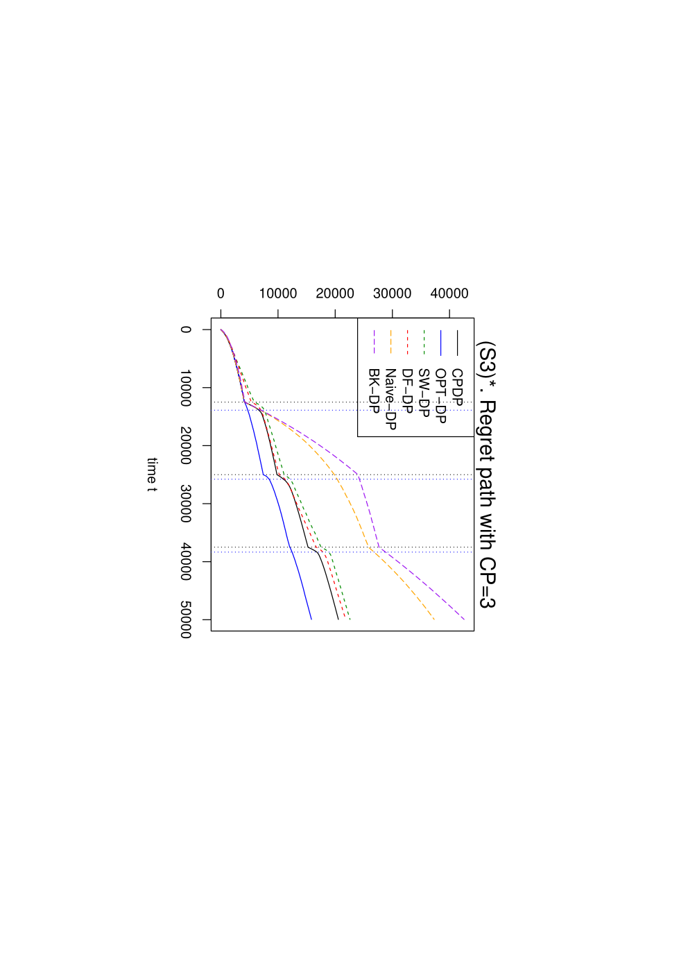
Refer to caption
Refer to caption
Refer to caption
Figure 9: Mean regret vs. TT under (S4) [left], (S5) [middle], (S6) [right] with λfix=0.2​log⁡(T​d)\lambda_{\mathrm{fix}}=0.2\sqrt{\log(Td)}.

G.3 Additional results for the auto loan dataset

Offline change-point detection algorithm: We run a standard model selection based offline change-point detection algorithm for logistic regression (Davis et al. 2006, Bai and Perron 2003, e.g.,) on {(yt,zt∗,pt)}t=150000\{(y_{t},z_{t}^{*},p_{t})\}_{t=1}^{50000}, which returns three change-points at t=12916,24986,37054.t=12916,24986,37054. In the following, we describe the algorithm, which estimates change-points based on optimizing a penalized likelihood function.

Given θ=(α,β),\theta=(\alpha,\beta), the logistic regression specifies that

𝔼⁡(yt|zt∗,pt)=ψ′​(α⊤​zt∗+β​pt),\mathbb{E}(y_{t}|z_{t}^{*},p_{t})=\psi^{\prime}(\alpha^{\top}z_{t}^{*}+\beta p_{t}),

where ψ′​(⋅)\psi^{\prime}(\cdot) is the logistic function.

Define 𝒯={𝝉:0=τ0<τ1<τ2<⋯<τK<τK+1=T,K∈ℕ}\mathcal{T}=\{\bm{\tau}:0=\tau_{0}<\tau_{1}<\tau_{2}<\cdots<\tau_{K}<\tau_{K+1}=T,K\in\mathbb{N}\} as the candidate set of all possible vectors of change-points. For a given change-point candidate 𝝉=(τ1,⋯,τK)\bm{\tau}=(\tau_{1},\cdots,\tau_{K}), the penalized likelihood function is defined as

F(𝝉)=−2∑k=0K[maxθ∑t=τk+1τk+1log(f(yt|zt∗,pt,θ))]+K(d+1)logT\displaystyle F(\bm{\tau})=-2\sum_{k=0}^{K}\left[\max_{\theta}\sum_{t=\tau_{k}+1}^{\tau_{k+1}}\log(f(y_{t}|z_{t}^{*},p_{t},\theta))\right]+K(d+1)\log T

where dd is dimension of (zt∗,pt)(z_{t}^{*},p_{t}) and f⁡(yt|zt∗,pt,θ)f(y_{t}|z_{t}^{*},p_{t},\theta) is the likelihood function of yty_{t} given zt∗,ptz_{t}^{*},p_{t} and θ.\theta. In other words, F⁡(𝝉)F(\bm{\tau}) is the BIC-based model selection criterion, where the first component is the summation of negative log-likelihood of each stationary segment and the second component is the BIC penalty for model complexity.

The change-point estimator is defined as

𝝉^=(τ^1,⋯,τ^K^)=\argmin𝝉∈𝒯​F​(𝝉),\displaystyle\widehat{\bm{\tau}}=(\widehat{\tau}_{1},\cdots,\widehat{\tau}_{\widehat{K}})=\argmin_{\bm{\tau}\in\mathcal{T}}F(\bm{\tau}),

which can be solved in O⁡(T2)O(T^{2}) operations via dynamic programming. We refer to Bai and Perron 2003 for more details.

Table 3: Summary of the auto loan dataset used in Section 5.3
Variable Type Description
apply Binary Indicator for eventual contract (dependent variable)
Price Continuous Price of the loan
Primary_FICO Continuous FICO score
Competition_rate Continuous Competitor’s rate
Amount_Approved Continuous Loan amount approved
onemonth Continuous Prime rate
Term Continuous Approved term in months
Tier Categorical Segmentation (1–7) based on FICO scores (defined by company)
rate Continuous Customer rate
CarType Categorical Type of car (new and used)
rate1 Continuous Rate relative to the prime rate
rel_compet_rate Continuous Rate relative to the competitor’s rate
mp Continuous Monthly payment
mp_rto_amtfinance Continuous Monthly payment over amount financed
partnerbin Categorical Segmentation based on loan partners
States Categorical Customer state