Waveguide QED with Quadratic Light-Matter Interactions
Abstract
Quadratic light-matter interactions are nonlinear couplings such that quantum emitters interact with photonic or phononic modes exclusively via the exchange of excitation pairs. Implementable with atomic and solid-state systems, these couplings lead to a plethora of phenomena that have been characterized in the context of cavity QED, where quantum emitters interact with localized bosonic modes. Here, we explore quadratic interactions in a waveguide QED setting, where quantum emitters interact with propagating fields confined in a one-dimensional environment. We develop a general scattering theory under the Markov approximation and discuss paradigmatic examples for spontaneous emission and scattering of biphoton states. Our analytical and semi-analytical results unveil fundamental differences with respect to conventional waveguide QED systems, such as the spontaneous emission of frequency-entangled photon pairs or the full transparency of the emitter to single-photon inputs. This unlocks new opportunities in quantum information processing with propagating photons. As a striking example, we show that a single quadratically-coupled emitter can implement a two-photon logic gate with unit fidelity, circumventing a no-go theorem derived for conventional waveguide-QED interactions.
I Introduction
The study of light-matter interactions is one of the main research pillars of quantum science. The implementation of systems where quantum emitters interact strongly with confined modes of the electromagnetic fields has allowed us to achieve an unprecedented level of control over quantum degrees of freedom Haroche and Raimond 2006; Gardiner and Zoller 2004. In the framework of cavity quantum electrodynamics (QED), the confinement of the electromagnetic field makes it possible to observe a coherent exchange of excitations between localized photonic modes and single quantum emitters Chang et al. 2014. Similarly, the coupling of quantum emitters to propagating fields can be strongly enhanced using waveguide structures, which confine photons to a one-dimensional environment Chang et al. 2018; Sheremet et al.. This setup, known as waveguide QED, has been realized in a variety of platforms such as atoms Reitz et al. 2013; Goban et al. 2015; Solano et al. 2017; Corzo et al. 2019 or quantum dots Arcari et al. 2014; Grim et al. 2022 coupled to photonic waveguides, as well as superconducting qubits Astafiev et al. 2010; Forn-Díaz et al. 2017; Liu and Houck 2017; Eder et al. 2018; Mirhosseini et al. 2019; Kannan et al. 2020a; Brehm et al. 2021; Scigliuzzo et al. 2022; Zanner et al. 2022 coupled to microwave transmission lines. Waveguide QED structures have a great potential to implement building blocks of quantum networks Lodahl 2017; Kimble 2008, since propagating photons are ideal to transport flying qubits over long distances while emitters can provide the strong quantum non-linearity necessary for quantum information processing. Therefore, there has been intense theoretical Fan et al. 2010; del Valle et al. 2012; González-Tudela et al. 2015; Shi et al. 2015; Ramos and García-Ripoll 2017; Ramos and García-Ripoll 2018; Mahmoodian et al. 2020; Trivedi et al. 2020 and experimental Stiesdal et al. 2018; Prasad et al. 2020; Le Jeannic et al. 2021; Kannan et al. 2020b; Hinney et al. 2021; Le Jeannic et al. 2022 research in the control and characterization of few-photon correlations generated by single quantum emitters, as well as in the implementation of photonic devices working at the few-photon level Hoi et al. 2011; Bennett et al. 2016; Scheucher et al. 2016; Nysteen et al. 2017; Uppu et al. 2021; Reuer et al. 2022; Yang et al. 2022.
In the vast majority of platforms, quantum emitters couple linearly, via dipolar interactions, to photonic or phononic modes. Such interactions support only the exchange of individual quanta—e.g. an atom decays emitting a single photon—. Transitions involving multiple quanta appear as higher-order processes and are therefore strongly suppressed. Only recently, it has been shown how to implement nonlinear couplings where a quantum emitter interacts with localized bosonic modes via the direct exchange of two excitation quanta (e.g. an atom decays emitting a photon pair). Often dubbed two-photon interactions, these quadratic light-matter couplings have been proposed in cavity QED settings such as superconducting qubits non-linearly coupled to quantum microwave resonators Felicetti et al. 2018a; Felicetti et al. 2018b; Bertet et al. 2005 or nanomechanical oscillators Zhou and Mizel 2006. Alternatively, quadratic couplings can also be effectively induced via parametric pumping and other simulation schemes intrinsic to superconducting circuits Ann et al. 2022, hybrid spin-nanomechanical oscillators Wang et al. 2016; Sánchez Muñoz et al. 2018, trapped ions Felicetti et al. 2015; Cheng et al. 2018; Puebla et al. 2019; Cong et al. 2020, and ultracold atoms Schneeweiss et al. 2018; Dareau et al. 2018. Notice that non-dipolar Goetz et al. 2018 couplings have already been observed using superconducting artificial atoms.
The rich quantum phenomenology arising in quadratic light-matter interactions motivates a fast-growing interest. For example, the two-photon quantum Rabi model is characterized by counter-intuitive spectral features such as the spectral collapse Travěnec 2012; Duan et al. 2016; Cong et al. 2019; Xie and Chen 2021, which can have direct observable consequences Felicetti et al. 2015; Felicetti et al. 2018b. Strong quadratic emitter-field couplings can induce high-order quantum optical nonlinear processes Felicetti et al. 2018a; Zou et al. 2020; Wang et al. 2021. Quantum phase transitions Garbe et al. 2017; Chen and Zhang 2018; Cui et al. 2019; Garbe et al. 2020; Cui et al. 2020; Ying 2021; Li et al. 2022 and quantum collective-emission phenomena Delmonte et al. 2021; Piccione et al. 2022 have also been analyzed. This phenomenology can be exploited in quantum-information applications such as non-classical state generation Villas-Boas and Rossatto 2019; Casanova et al. 2018; González-Gutiérrez and Torres 2019, quantum sensing Ying et al. 2022, cat-qubit stabilization Gautier et al. 2022 and qubit-noise spectroscopy Mutter and Burkard 2023. However, so far quadratic light-matter couplings have only been studied in the case of localized bosonic modes.
In this work, we develop a quantum optics theory to describe a single quantum emitter interacting quadratically with the photons that propagate along a one-dimensional waveguide. We study this problem with a two-photon scattering theory based on a Wigner-Weisskopf approach and the Born-Markov approximation. We derive the general form of the scattering matrix, including semi-analytical solutions for arbitrary photonic input states and full analytical solutions for Gaussian inputs. Applying this theory, we unveil observable features of the emitter’s response that are fundamentally different with respect to conventional waveguide QED setups (see Fig. 1). These include (i) the spontaneous emission of correlated biphoton states, (ii) the strong interaction with spectrally narrow two-photon pulses, and (iii) full transparency to single-photon inputs. Finally, we show that these effects can be exploited in quantum information applications, designing a deterministic controlled-phase gate that acts on pairs of propagating photons with perfect fidelity. This result seems to contradict a famous no-go theorem for photonic gates Shapiro 2006; Gea-Banacloche 2010; Nysteen et al. 2017. However, it is the use of quadratic interactions that allows us to eliminate the wavepacket distortions that are intrinsic to the localized non-linearities induced by linear light-matter coupling Nysteen et al. 2017. The proposed gate is based on dual-rail encoding, which is of increasing relevance for superconducting quantum-computing applications Teoh et al. 2022. All results discussed in this work can be implemented using state-of-the-art superconducting quantum emitters Felicetti et al. 2018a; Felicetti et al. 2018b; Bertet et al. 2005; Ann et al. 2022 interacting with propagating microwave fields or nanomechanical oscillators Zhou and Mizel 2006 and we expect that similar regimes will soon be achievable with solid-state Wang et al. 2016; Sánchez Muñoz et al. 2018 or atom-based Felicetti et al. 2015; Cheng et al. 2018; Puebla et al. 2019; Cong et al. 2020; Schneeweiss et al. 2018; Dareau et al. 2018 nanophotonic devices.
The work is structured as follows. In Sec. II, we develop a general theory for the scattering of pairs of photons by a single quantum emitter interacting quadratically with a one-dimensional waveguide. In Sec. III, we derive consequences from this theory, such as the two-photon spontaneous emission law and the two-photon scattering probabilities. We derive general bounds for the scattering cross-section valid for arbitrary photon-pair (biphoton) input states. We then consider specific examples for spontaneous emission and for the scattering of biphoton states with Gaussian and Lorentzian frequency distributions. In Sec. IV, we provide a striking example of application in quantum-information tasks, showing how to design a controlled-phase gate with unit fidelity. In Sec. V, we discuss possible physical implementations of the considered model. In Sec. VI, we provide conclusions and the outlook for future directions.

II Scattering theory for two-photon interactions
This section introduces a new scattering theory for two-photon states impinging on a quadratically-coupled quantum emitter. It describes the model’s Hamiltonian (II.1), the derivation of the scattering equations using the Wigner-Weisskopf formalism (II.2), and the computation of the two-photon scattering matrix under the Markov approximation (II.3).
II.1 Model
We consider a two-level quantum emitter with general quadratic coupling to a continuum of bosonic modes in a one-dimensional waveguide. Under the rotating-wave approximation, the system Hamiltonian can be written as (),
| (1) |
Here, and () are the resonance frequency and the raising (lowering) operator of the emitter, respectively. The operator () annihilates (creates) a waveguide photon with frequency and propagating direction . We denote with the function that gives the quadratic coupling strength between the emitter and the field frequency components. Note that Eq. (II.1) is over-parametrized. This is because the relation implies that all vector elements appear twice in the summation and integration. Therefore, we can arbitrarily set the symmetric condition , holding for any , , and . We will keep the coupling function as general as possible in the derivation, specifying it only in the examples, in order to identify the intrinsic properties of the quadratic coupling. The scattering theory that we develop is applicable to different experimental implementations of the model.
II.2 Wigner-Weisskopf ansatz
The Hamiltonian in Eq. (II.1) commutes with the operator . This is a continuous-symmetry generator associated with the conservation of the weighted number of excitations Felicetti et al. 2015. This conservation law implies that the whole dynamics can be described using a Wigner-Weisskopf ansatz wavefunction with a fixed number of (weighted) excitations as defined by . In the vacuum sector or in the sector with individual photons, this dynamics is trivial: in both cases, the photonic states are decoupled from the emitter, which is transparent to individual photon states.
Consequently, we may focus on solving the scattering problem for input states with either two incoming photons and an emitter in the ground state, or an excited emitter in the vacuum. The most general such state,
| (2) |
is constructed by creating excitations on top of , the tensor product between the bosonic vacuum and the emitter’s ground state. The two-photon Wigner-Weisskopf state is normalized as
| (3) |
and it holds that for any , , , .
The Wigner-Weisskopf ansatz (II.2) describes a solution to the Schrödinger equation, , provided the coefficients satisfy a set of coupled, linear ordinary differential equations:
| (4) | ||||
| (5) |
It is convenient to reparameterize the wavefunction’s element using the sum and difference of photon frequencies, and , as and .
At this stage, let us introduce the Markovian approximation, assuming that the emitter will spontaneously decay, releasing photons to the waveguide at a rate that is much slower than its intrinsic frequency, . In this limit one can formally solve Eq. (5) and replace the solution into Eq. (4) to obtain (see App. A.1):
| (6) |
The total spontaneous emission rate is self-consistently defined as
| (7) |
In the standard Markovian approach with linear interactions, the decay rate depends on the frequency of the emitted photons, although this dependency is usually weak or ignored Gardiner and Zoller 2004. In the case of quadratic light-matter interactions, the decay rate depends on the coupling strength evaluated at the two-photon resonance, i.e. at , and integrated over frequency differences . We can assume that the coupling strength does not change significantly with , at least in a band of frequencies around , but we cannot fully eliminate the dependency on , thus . This dependency may be factored into a product of emission rates and an envelope , i.e.
| (8) |
We consider to be the dominant energy scale, that is we take for the upper integration limit in Eq. (7). This corresponds to assuming that the coupling function quickly decays with . Then, we take to be a bell-shaped function normalized to 1 in the -norm, i.e. 11 1 The -norm is defined as . This convenient normalization implies that the function encodes the difference-frequency dependence of the coupling strength, but it does not affect the total emission rate . As we will see in the following, the explicit dependence on has highly non-trivial consequences on the scattering phenomenology and on potential applications.

II.3 Two-photon scattering matrix
The scattering matrix connects linearly the amplitude coefficient of the input photons with the output field at asymptotic times , when all the interaction with the quantum emitter has ceased. As explained in App. A.2, it is derived by integrating Eq. (5) using the initial and the final times as boundary conditions and equating the results. We obtain:
| (9) |
where we defined . This quantity may be obtained from the Fourier transform of Eq. (II.2), i.e.
| (10) |
assuming that the emitter is initially in the ground state and that there is a large temporal separation between the input and the output events. More precisely, we require that , so that the emitter is completely decayed at the time in which the output state is formally defined . For simplicity, in the following we consider the narrow-bandwidth limit and extend the integration region to in Eq. (10) (see App. A.2). This assumption is not strictly needed to obtain semi-analytical results.
For the sake of clarity, let us first write the scattering relations for a fixed propagation direction of the input field along the waveguide. In other words, we set for some fixed and , where is a Kronecker delta. In this way, we can remove the summation in the direction index in Eq. (10). This assumption will be dropped in the final expression of the scattering matrix. After all these manipulations, the output and input states are related through
| (11) |
As in the standard case of dipolar interactions, the output field is the interference between the input biphoton state (first line) and the two photons re-emitted by the atom (second line). Also as in standard waveguide QED, the Markovian approximation manifests itself in the Lorentzian dependency with respect to the total energy of the input field . However, differently from the dipolar case, for quadratic interactions the re-emitted field depends on the relative frequency through the interaction envelope . In the next sections, we will explore the consequences of this relationship. Let us now write a general relation for the two-photon scattering matrix.
Proposition 1.
[Scattering matrix]
Consider a quadratic interaction between bosonic modes and a two-level emitter, defined by the Hamiltonian in Eq. (II.1), under Markovian approximation . Given a two-photon input state as in Eq. (II.2), the probability amplitudes at a time such that are
| (12) |
where a summation is implicit over the repeated indexes and . The term is a generic element of the scattering matrix, which can be expressed as
| (13) |
where we defined
| (14) |
In Eqs. (12) and (13), we identify that the integration with plays the role of a projection onto a specific biphoton distribution . The action of the scattering matrix onto the input state is better understood if we explicitly separate the parallel and orthogonal components to as
| (15) |
with
| (16) |
The scattering relation can then be rewritten as
| (17) |
The orthogonal component is unperturbed by the quantum emitter. The parallel component experiences a transformation which is analogous of the scattering phase for a single photon in waveguide QED with linear Markovian interaction Fan et al. 2010.
III Paradigmatic cases
In this section, we study the phenomenology of spontaneous emission (III.1) and two-photon scattering (III.2), analyzing the cross-section and the spectral features of the output channels. In the case of scattering of biphoton states, we provide general bounds on the scattering probabilities which hold for arbitrary frequency distributions of the input. We then focus on the Gaussian case, where we are able to give explicit analytical solutions for the scattering matrix and gather physical intuition on the features of the scattering problem. We also reproduce the analysis in the semi-analytical case of Lorentzian coupling function, which confirms that the results of the Gaussian case are valid for biphoton states of high experimental relevance.
III.1 Spontaneous emission
When we excite the quantum emitter in a waveguide without photons and both interact via Eq. (II.1), we expect the emitter to relax to the ground state emitting two photons. We can use the Wigner-Weisskopf theory [see Eq. (II.2)] to derive the frequency distribution of the emitted photons at asymptotic times. In the Markovian regime, the amplitude of the emitter’s excited state decays exponentially with the rate introduced in Eq. (7):
| (18) |
The emitted photon wavepacket in frequency space at long times is recovered by inserting Eq. (18) into Eq. (9). This wavefunction,
| (19) |
depends on the sum and on the difference of frequencies . This profile resembles the Lorentzian lineshape that is characteristic of Markovian dynamics, where the wavepacket is centered around the total energy of of the incoming photons. However, the actual wavepacket is now shaped by the dependence of the interaction on the relative frequency of the photons . This is a general result that can be applied to very different experimental scenarios.
Example: Gaussian and Lorentzian coupling functions– As an example, let us compute the spectrum of the spontaneously emitted photon pairs in Eq. (19), assuming two different frequency distributions for the coupling function. The first coupling function is Gaussian with zero mean and variance , i.e.
| (20) |
For comparison, we consider also a Lorentzian distributed coupling
| (21) |
This gives us an expression for via Eq. (19). In Fig. 2, we plot the emission rate for three different values of , in the isotropic case where . Notice that, unless a non-isotropic emitter or a chiral waveguide is considered Lodahl et al. 2017, there are three possible output channels, such that the photon pairs are emitted on the same direction or they can split. The frequency distribution is shown in Fig. 2 and it is the same for the three possible channels.
Summarizing, similarly to standard linear couplings the decay of the emitter excitation is exponential. Strong elements of novelty are: (i) Spontaneous decay of a single emitter results in the generation of a photon pair. (ii) The emitted biphoton state has a non-trivial frequency distribution, which is Lorentzian in the sum-frequency variable (main diagonal in Fig. 2, width set by the total decay rate ), while it reproduces the coupling function in the difference-frequency variable [anti-diagonal in Fig. 2, width set by the full width at half maximum, FWHM, of ]. (3) Interestingly, it is possible to generate frequency-correlated or anticorrelated photon pairs by changing the ratio between the total emission rate and the FWHM of the coupling function .
III.2 Scattering of two-photon inputs

Let us discuss the phenomenology that appears in the scattering dynamics computed in Sec. II.3. As sketched in Fig. 1, for two copropagating input photons , there are three possible outcomes classified by the output directions: (i) reflection (), (ii) transmission () and (iii) splitting (), depending on whether both directions are preserved or reversed, or become opposite to each other. The respective scattering probabilities integrated over the complete frequency range are
| (22) |
These values depend on the particular input field, but they exhibit general symmetries and constraints that can be derived from Prop. 1.
Let us find an upper bound to the reflection probability under reasonable assumptions on the input state. This corresponds to maximizing Eq. (22) for . Let us assume the atom to be initially in its ground state and the input field probability amplitude to be separable in and , i.e.
| (23) |
where and are complex functions normalized in the -norm, i.e. . By using the Cauchy-Schwarz inequality in Eq. (12), we obtain
| (24) |
The inequality in Eq. (24) is saturated if and only if , that is when the frequency distribution of the input field matches the coupling function . Inserting Eq. (24) into Eq. (22) and using Holder’s inequality, we obtain that the reflection probability is bounded by
| (25) |
This inequality is saturated when the bandwidth of the input field —measured as the FWHM or by some other means—is much narrower than the emitter’s natural linewidth .
We can also derive exact expressions for the maximal achievable rates of splitting and transmission processes, defined as
| (26) | ||||
| (27) |
While in waveguide QED with linear interactions a single emitter can perfectly reflect a single photon Hoi et al. 2011, the perfect two-photon reflection by a quadratically-coupled emitter is only possible when the splitting process is suppressed, i.e. and . In the case of isotropic interactions , this is thus not possible. Here, even for optimal frequency-matched input , one obtains , and .

Example: Gaussian wavepackets– Let us discuss a scattering experiment with Gaussian couplings and Gaussian input wavepackets that has analytical solutions and which provides insight that is extensible to other situations, e.g., the Lorentzian case shown in App. B. Without loss of generality, we use the isotropic Gaussian coupling function with variance from Eq. (20). The input state is formed by two Gaussian wavepackets with frequencies , propagating along the same direction with identical widths . The state is separable both on the individual photons’ frequencies and the canonical variables
| (28) |
We can now use the scattering matrix formalism to retrieve the expression of the output amplitude probabilities (see Prop. 1). Indeed, using Eq. (12) and Eq. (20), we find the frequency distribution of the field for the different output channels
| (29) |
Let us now analyze the phenomenology described by this analytical result, focusing on the spectral properties of the output field and the scattering probabilities.
In Fig. 3, we plot the spectral distribution of the reflected (), split () and transmitted () states, derived from Eq. (III.2) for two values of . The distribution of the scattered/split photons is strongly anti-correlated in frequency, even though the input state was a separable one. A careful observation of the formulas reveals how the output field can be tailored by choosing the input state and by engineering the coupling function. In the sum-frequency variable [main diagonal in Fig. 3], the distribution has a Lorentzian shape whose width is established by the intensity of the light-matter coupling strength . A larger value of the parameter translates into a larger FWHM for the reflected frequency distribution. In the difference-frequency variable [anti-diagonal in Fig. 3], the distribution has a Gaussian shape whose width depends on the widths of the input distribution and of the coupling function .

In Fig. 4, we analyze how the total reflection rate depends on the input frequency distribution and the emitter properties. We plot as a function of the ratio between the standard deviation of the coupling function [see Eq. (20)] and the standard deviation of the sum-frequency distribution of the input field [see Eq. (28)]. As expected, the scattering rate is maximal when the input frequency distribution matches the coupling function, a specific occurrence of the general results derived in Sec. II.3. By probing different emission rates , Fig. 4 also confirms that the upper bound on the reflection probability is attainable when the width of the input frequency distribution is small compared to the emitter line width, .
III.3 Entanglement generation
From the phenomenological analysis of Sec. III.1 and Sec. III.2, one can easily infer that two-photon states scattered or spontaneously emitted by a quadratically-coupled emitter have non-trivial entanglement properties. In general, the scattered/emitted states are hyper-entangled, i.e. non-classical correlations are present both in the position and in the frequency degrees of freedom. For the sake of brevity, we will focus here on entanglement generated in the (continuous) frequency variable. We consider a specific measurement setting relevant for practical experiments and applications such as quantum key distribution. Let us take the case of a spontaneously emitted two-photon state, which can be obtained by plugging the result of Eq. (19) in the definition of the state Eq. (II.2). We consider the setup shown in Fig. 5(a), that is we take the post-selected state in which the photons are emitted in opposite directions, i.e.
| (30) |
where is a renormalization factor and where we have re-expressed the output frequency distribution as a function of the frequencies of the output photons and . Bipartite entanglement in a continuous variable such as the frequency can be fully characterized with a Schmidt decomposition Lamata and León 2005; Fabre et al. 2022. However, here we consider a simpler approach that is of direct experimental relevance. We identify two discrete frequency modes by applying frequency filters, defined by the functions . The effect of the filters is modeled by applying the following transformation to the state distribution:
| (31) |
We choose the filters to have two narrow transmission windows, so that they are well approximated by the sum of two Dirac deltas centered around frequencies and , . After the filters, the (post-selected state) can be written as
| (32) | |||||
where the first(second) quantum number in the ket notation encodes the frequency of left(right) propagating photons, that is .
We can now characterize the entanglement of the two-qubit state defined by Eq. (32). As entanglement measure we use the entanglement entropy defined as , where we defined the reduced density operator , obtained by tracing out system 2 to the global state of Eq. (32). In Fig. 5(b) and (c) we analyze the behavior of the entanglement for different system parameters, considering the frequency distribution of Eq. (19) with the Lorentzian coupling function of Eq. (21). We take the filters to be centered around frequencies symmetric with respect to the atomic resonance, that is we fix and in Eq. (32). In Fig. 5(b) we show that the entanglement entropy grows with the frequency-offset , until it saturates to a plateau. This is consistent with the intuition gathered by looking at Fig. 2. Indeed, the output frequency distribution is separable close to the resonance condition, while positive or negative correlations can be observed far from resonance. To further characterize correlations, in Fig. 5(c) we show the entanglement entropy as a function of the ratio between the width of the coupling function and the total emission rate . For we observe a minimum of the entanglement entropy, as the frequency distribution is approximately separable [see Fig. 2]. For small values of [Fig. 5(d)] the state is strongly correlated, and in the limit the state asymptotically approaches a Bell state . On the contrary, for large values of [see Fig. 5(e)], the output photons are anticorrelated in frequency and the state asymptotically approaches the following Bell state . Therefore, quadratically-coupled atoms represent a compelling tool to generate frequency-entangled states, which are relevant for a variety of quantum-information applications Fabre et al. 2022; Lyons et al. 2018; Chen et al. 2019; Fabre and Felicetti 2021. In the following section, we provide another striking example of potential applications.
IV Ideal controlled-phase gate for propagating photons
Let us now provide a compelling application of this phenomenology in quantum computing tasks. We consider a controlled-phase gate implemented on qubits defined with a dual-rail encoding, which is of increasing relevance for quantum computing with superconducting circuits Teoh et al. 2022. In particular, we consider an encoding where each qubit is defined as a single photon distributed along two propagating modes and , such that the logical states are encoded as and . Regardless of the physical encoding, a c-phase (or control-Z) gate is defined by the transformation
| (33) |
where and denote the control and signal logical qubits, respectively.
It has been shown in Ref. Nysteen et al. 2017 that, by first principles, it is impossible to implement this gate with unit fidelity using a single (point-like) two-level quantum emitter as the nonlinear element. The reason is that a distortion of the wavefunction frequency distribution is unavoidably introduced, as conflicting requirements on the input state should be imposed for the single- and two-photon scattering events. This no-go theorem has been derived assuming standard linear interactions. There are alternative proposals to circumvent such an intrinsic limitation, but they come at the cost of using multi-level artificial atoms Zheng et al. 2013, an array of many emitters Brod and Combes 2016, or an active time-dependent modulation of the coupling strength Heuck et al. 2020.
In the following, we propose a straightforward scheme that can overcome this limitation and implement a passive protocol for a c-phase gate with (in principle) unit fidelity, by using a single quadratically coupled two-level emitter per path. The scheme (sketched in Fig. 6) is composed of four semi-open waveguides (two for the control and two for the signal photons), each encoding a state of one of the two logical qubits. A balanced beam-splitter (BS), represented as a directional coupler in the sketch, connects the and paths. As the BS is traversed back and forth, it does not modify the logical input states. As a result, since quadratically coupled emitters are transparent to single-photon signals, it can be shown by direct inspection that the first three operations of Eq. (IV) are correctly implemented. When the input state is , after the first passage in the BS the state will be , i.e. the photons will come out from the same path. The role of the BS is then to send both photons toward the same emitter if and only if the input state is .
Let us analyze the process in which two photons (or equivalently ) scatter from the quadratically coupled emitters. We will compute which wavefunction of the two input photons maximizes the gate fidelity, studying the problem in frequency space. When the emitter is placed at the end of a semi-infinite waveguide, all photons are reflected, and the probability amplitudes of the output field are given by Prop. 1 with , and the only non-zero coupling term is , with . From Eq. (7), it follows that . As shown in Sec. III.2, the optimal interaction is achieved when the input state wavefunction in frequency space matches the distribution of the coupling. Consequently, we assume a biphoton input state given by , where . Following Prop 1, the output field is
| (34) |
where we dropped the propagation-direction indexes for the sake of brevity. Note how the output field equals the input field times a Lorentzian (in square brackets) in , which in the limit of approaches . We may use this limit to implement a c-phase gate, by imposing that the input state is a Bell-shaped function, with FWHM , concentrated around the resonance frequency . In the limit of narrow photons, , the output field acquires the desired nonlinear phase , up to a phase common to all logical input states.


Let us now analyze the performance of the controlled-phase gate, estimating the worst-case fidelity over all possible logical qubit states . In a loss-less waveguide, the worst-case fidelity is defined as Nysteen et al. 2017
| (35) |
where is the ideal c-phase gate and are the actual operation experienced by the single and biphoton states. In our setup, only the two-photon state experiences a nontrivial scattering. We may thus write
| (36) |
with and given by Eq. (34). Inserting Eq. (IV) into Eq. (35), we obtain a formula that only depends on the overlap
| (37) |
In Fig. 7, we show the worst-case gate logarithmic infidelity as a function of expressed in units of the input FWHM. We compared two different relevant input cases: real Normal distributed and real Lorentzian distributed. Both distributions are centered on the resonance frequency and have the same FWHM. We observe a steeper slope for the Normally distributed with respect to the Lorentzian one, due to the higher variance of the latter. Most importantly, in the limit of narrow inputs, FWHM, the worst-case gate fidelity approaches 1, thus overcoming the intrinsic limitation Nysteen et al. 2017 found when considering linear interactions. This unanticipated result is of high conceptual value, as part of a prototypical analysis based of an effective model. An assessment of the fidelity achievable in practice should be done considering a specific device and keeping into account the corresponding main sources of dissipation and decoherence.
V Discussion on physical implementations
Let us now provide comments on possible physical implementations of the considered model. There are two main approaches to implement quadratic interactions in the context of cavity QED. The first one consists in designing effective implementations, or analog quantum simulations, where an external driving is used to selectively activate pump-induced interactions. This approach can be applied to a broad variety of quantum platforms and it was considered to design quadratic interactions first for atomic systems Felicetti et al. 2015; Cheng et al. 2018; Puebla et al. 2019; Cong et al. 2020; Schneeweiss et al. 2018; Dareau et al. 2018 and then in solid state devices Ann et al. 2022; Wang et al. 2016; Sánchez Muñoz et al. 2018. The second approach consists in engineering genuine quadratic couplings, such that the nonlinearity of the interaction is intrinsic and the exchange of excitations is not mediated by external drivings. Genuine implementations have been designed for superconducting quantum circuits Felicetti et al. 2018a; Felicetti et al. 2018b; Bertet et al. 2005 and nanomechanical resonators Zhou and Mizel 2006. In particular, the most promising platform to implement the proposed controlled-gate is circuit QED Blais et al. 2021, where decoherence and noise sources can be typically controlled within the 1%. In this framework, it was shown that it is possible to engineer a genuine quadratic qubit-cavity coupling Felicetti et al. 2018a while fully inhibiting the linear coupling. It was also shown that a similar implementation can even be pushed into the ultrastrong coupling regime Felicetti et al. 2018b. Such proposals are based on a flux qubit inductively coupled to a SQUID device, where the latter is operated in a weakly-nonlinear regime and is well approximated by a harmonic mode.
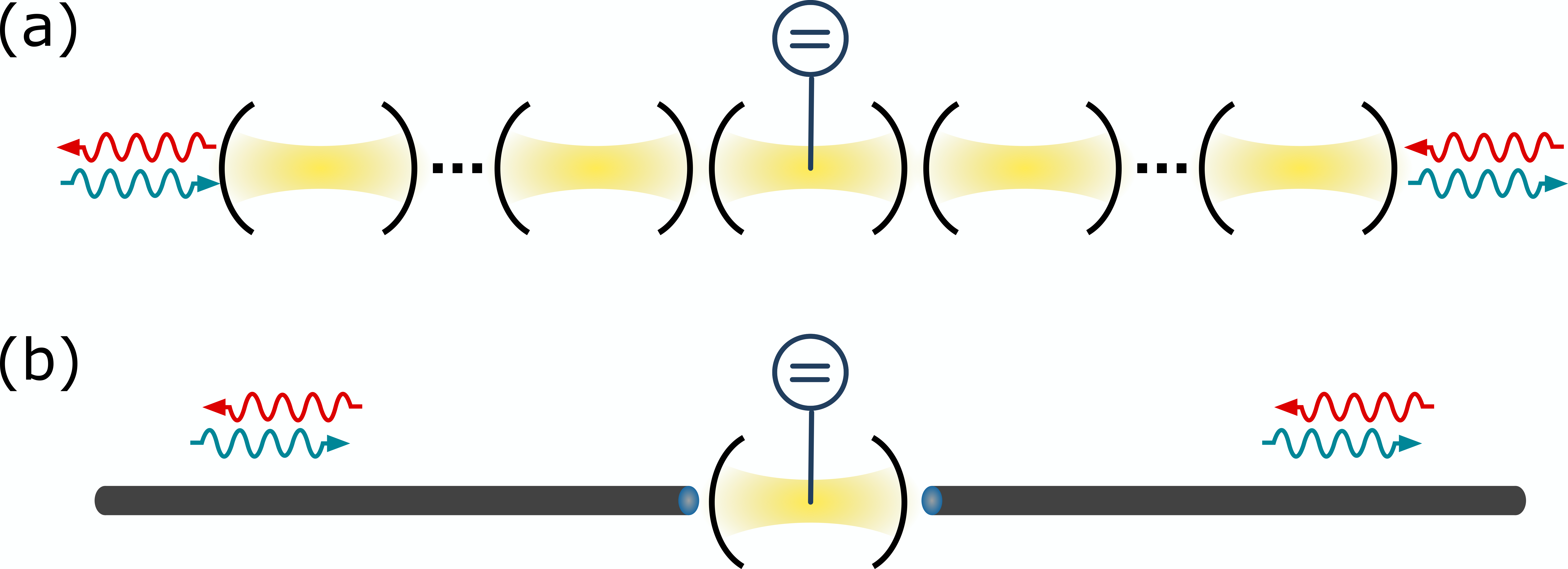
Currently, it is therefore well understood how to design genuine implementations of quadratic interactions between a quantum emitter and localized harmonic modes. Going a step further, here we envision two ways in which these cavity QED settings could be directly generalized to implement quadratic couplings to propagating modes: (i) The most straightforward generalization is shown in Fig. 8(a) and consists in implementing an array of coupled cavities which supports propagating modes Ramos et al. 2016; Calajó et al. 2016. A quadratically-coupled emitter could be added using known designs into one of the resonators of the array. In this case, the quadratic coupling function to propagating modes would depend on the collective mode structure of the resonator array, and in the weak coupling limit we expect the effective dynamics to be Markovian Ramos et al. 2016 as assumed in this work. (ii) An alternative solution is shown in Fig. 8(b) and consists in considering a quadratic atom-resonator system in the bad cavity limit, where the resonator dissipation rate is large compared to the coupling so that its modes can be adiabatically eliminated Auffèves-Garnier et al. 2007; Reiter and Sørensen 2012. In this case, we expect an effective quadratic coupling with Lorentzian-like distribution between the artificial atom and the propagating modes of waveguides coupled to the leaky resonator.
These two solutions allow the implementation of the considered model with known results. A possible solution that would require further analyses consists in generalizing the superconducting circuit designs Felicetti et al. 2018a; Felicetti et al. 2018b to a native waveguide-QED setting. In the simplest case, such a configuration could consist in a superconducting transmission-line waveguide that is galvanically coupled to a flux qubit through a SQUID. More complex configurations could be designed considering SQUID-based metamaterials. A detailed analysis of any of these implementations should be performed considering the microscopic modeling of the specific platform and this is outside the scope of this paper.
VI Conclusions and outlook
This work introduces the study of quadratic light-matter couplings in the field of waveguide QED. We have developed a general scattering theory with a broad range of applicability to solid-state and atomic quantum technologies. The predicted phenomenology is fundamentally different from what is observable with standard dipolar couplings and it bears great potential for quantum information applications. Remarkably, we show that a single quadratically coupled emitter can overcome a well-known no-go theorem and implement a controlled-phase gate on flying qubits with unit fidelity. Let us discuss the future perspectives in this novel research line, focusing first on the observation of an unconventional quantum phenomenology and then on the potential for quantum information applications.
In the framework of waveguide QED, quadratically-coupled emitters can be embedded in very different setups and configurations. For instance, the placement of artificial atoms in arrays with sub-wavelength spacing can be used to enhance/inhibit their individual emission rate and scattering properties, both in standard and chiral waveguides. The emergence of collective effects arising from many quadratically-coupled emitters has so far been studied only in the context of cavity QED Delmonte et al. 2021; Piccione et al. 2022. Nonlinear waveguide QED devices can also undergo interaction-induced phase transitions Iorsh et al. 2020; Sedov et al. 2020. Alternatively, quadratically coupled emitters can be used as nonlinear mirrors that confine multiphoton states, by analogy with similar studies in the dipolar coupling regime Chang et al. 2012. Furthermore, the quadratic coupling in waveguide-QED setups can be pushed into the non-Markovian or even in the ultrastrong-coupling regime, requiring the development of new theoretical and numerical tools Forn-Díaz et al. 2017 and opening the door to new correlated phases and quantum phase transitions. Finally, nonlinear couplings can also be combined with the framework of giant atoms Kockum 2021.
As demonstrated in this work, quadratic light-matter couplings are a compelling tool to process quantum information encoded in propagating photons. This possibility should be thoroughly addressed considering each specific experimental setting, with a detailed microscopic model of the system and realistic noise sources. The most interesting case is provided by superconducting quantum circuits, for which the dual-rail encoding is of high relevance for quantum computing Teoh et al. 2022. Finally, besides gates in the dual-rail encoding, quadratic light-matter couplings can be used to deterministically generate propagating biphoton states or to implement highly non-trivial photon subtraction processes. The possibility of tailoring the spectral features of emitted/scattered biphoton states paves also the way to the generation of entanglement in the time-frequency domain, which is relevant for quantum computation Fabre et al. 2022 and sensing Lyons et al. 2018; Chen et al. 2019; Fabre and Felicetti 2021 applications.
Acknowledgements.
We thank Francesco Ciccarello and Luca Leonforte for insightful discussions. U.A. and R.D. acknowledge support from the Academy of Finland, grants no. 353832 and 349199. Work in Madrid has been supported by the European Union’s Horizon 2020 FET-Open project SuperQuLAN (899354), Proyecto Sinergico CAM 2020 Y2020/TCS-6545 (NanoQuCo-CM), and the CSIC interdisciplinary Thematic Platform (PTI+) on Quantum Technologies (PTI-QTEP+) T.R. further acknowledges support from the Ramón y Cajal program RYC2021-032473-I, financed by MCIN/AEI/10.13039/501100011033 and the European Union NextGenerationEU/PRTR.
Appendix A Wigner-Weisskopf Theory
In this section, we provide a detailed derivation of the scattering matrix (Prop. 1) starting from the system of coupled differential equations for the amplitude probability coefficients in Eq. (4) and Eq. (5).
A.1 Markovian approximation
We start by solving formally the differential equation for the field amplitude probability coefficient :
| (38) |
Inserting this result in Eq. (4) allows us to decouple the system of equations and find a linear self-consistent differential equation for :
| (39) |
The last term in Eq. (A.1) can be further simplified. First, we change the integration variables defining , and , so that
| (40) |
Then we rewrite the integral as
| (41) |
where we have used and we have defined the kernel
| (42) |
So far the treatment is exact. Now we perform the Markovian approximation on the basis of two assumptions. First, we assume the coupling strength to be weak with respect to the emitter frequency . First-order perturbation theory allows us to rewrite the solution of Eq. (A.1) as , where is a slowly-varying function of time. Second, we point out that, if the coupling strength has a weak dependence on , the Kernel is a rapidly-decaying function. Note that indeed, in the limit in which the coupling is flat in frequency, the Kernel is proportional to a Dirac delta in time. So, if the coupling strength is perturbative and sufficiently smooth with respect to , we can approximate as a constant in the short time interval in which is non-vanishing. Accordingly, we can set in the time integral in Eq. (A.1) and recombine the terms so that
| (43) |
Note that for any specific form of the coupling strength, the integral in the last equation is now explicit and it can be evaluated by analytical or numerical means. However, to have a general analytical expression, we can take a further step and extend to infinity the upper limit of integration in Eq. (43). This corresponds to assuming that the Kernel correlation length is zero (which is standard in the Markov approximation, as it is exactly true when the coupling strength is natively constant with respect to ). Under this limit, performing the time-integration in Eq. (A.1), we obtain
| (44) | ||||
| (45) |
where we have defined the total emission rate as
| (46) |
We have also defined the Lamb shift
| (47) |
which is a small shift in the emitter resonance frequency. Here and in the main text, we absorb in the definition of , as in most cases the experimental characterization of the emitter frequency already includes the Lamb shift. Now that all the terms in Eq. (A.1) have been simplified, we are able to write a compact expression for the atom amplitude probability differential equation [Eq. (II.2) in the main text],
| (48) |
where for convenience we have used the relation
| (49) |
and , .
A.2 Scattering states
As done in Eq. (A.1), we can formally solve for setting the initial conditions for a time :
| (50) |
Subtracting Eq. (A.1) from Eq. (A.2), we find an input-output relation for the field before () and after () the scattering event:
| (51) | ||||
where we switched to the frequency-sum and difference variables and we have used that . We now take the Fourier transform of Eq. (A.1) [or Eq. (II.2)] and integrate by parts the left side, assuming that . We obtain
| (52) |
where we have used that, for , we can approximate . Finally, for the output state we find
| (53) | ||||
In the main text, we consider the narrow-bandwidth limit and extend to infinity the range of the integration over in the previous expression. This corresponds to assuming that the input distribution is non-vanishing only in a region around a central frequency which is of the order of (for two-photon interactions the input photons are resonant when the sum of their frequencies matches the emitter frequency). We also remind that is bell-shaped and non-zero only for .
Appendix B Lorentzian case
In Sec. III.2, we have presented results for the scattering of two-photon states in the Gaussian case, which can be analytically solved and allows one to understand the fundamental features of the two-photon scattering problem on a quadratically-coupled emitter. Let us now show that those features are not modified in the case of Lorentzian coupling functions [see Eq. (21)], which are more frequently encountered in realistic physical systems. This case can be solved semi-analytically using the results of Prop. 1, by numerically integrating Eq. (12). The results are presented in Fig. 9 and good qualitative agreement is found with the Gaussian case presented in Fig. 3.
References
- Haroche and Raimond (2006) S. Haroche and J.-M. Raimond, Exploring the Quantum: : Atoms, Cavities, and Photons (Oxford University Press, 2006).
- Gardiner and Zoller (2004) C. Gardiner and P. Zoller, Quantum Noise (SpringerVerlag, Berlin, 3rd Ed., 2004).
- Chang et al. (2014) D. E. Chang, V. Vuletić, and M. D. Lukin, Nat Photon 8, 685 (2014).
- Chang et al. (2018) D. E. Chang, J. S. Douglas, A. González-Tudela, C.-L. Hung, and H. J. Kimble, Rev. Mod. Phys. 90, 031002 (2018).
- (5) A. S. Sheremet, M. I. Petrov, I. V. Iorsh, A. V. Poshakinskiy, and A. N. Poddubny, arXiv:2103.06824 .
- Reitz et al. (2013) D. Reitz, C. Sayrin, R. Mitsch, P. Schneeweiss, and A. Rauschenbeutel, Phys. Rev. Lett. 110, 243603 (2013).
- Goban et al. (2015) A. Goban, C.-L. Hung, J. D. Hood, S.-P. Yu, J. A. Muniz, O. Painter, and H. J. Kimble, Phys. Rev. Lett. 115, 063601 (2015).
- Solano et al. (2017) P. Solano, P. Barberis-Blostein, F. K. Fatemi, L. A. Orozco, and S. L. Rolston, Nat Commun 8, 1857 (2017).
- Corzo et al. (2019) N. V. Corzo, J. Raskop, A. Chandra, A. S. Sheremet, B. Gouraud, and J. Laurat, Nature 566, 359 (2019).
- Arcari et al. (2014) M. Arcari, I. Söllner, A. Javadi, S. Lindskov Hansen, S. Mahmoodian, J. Liu, H. Thyrrestrup, E. H. Lee, J. D. Song, S. Stobbe, and P. Lodahl, Phys. Rev. Lett. 113, 093603 (2014).
- Grim et al. (2022) J. Q. Grim, I. Welland, S. G. Carter, A. S. Bracker, A. Yeats, C. S. Kim, M. Kim, K. Tran, I. Vurgaftman, and T. L. Reinecke, Phys. Rev. B 106, L081403 (2022).
- Astafiev et al. (2010) O. Astafiev, A. M. Zagoskin, A. A. Abdumalikov, Y. A. Pashkin, T. Yamamoto, K. Inomata, Y. Nakamura, and J. S. Tsai, Science 327, 840 (2010).
- Forn-Díaz et al. (2017) P. Forn-Díaz, J. J. García-Ripoll, B. Peropadre, J.-L. Orgiazzi, M. A. Yurtalan, R. Belyansky, C. M. Wilson, and A. Lupascu, Nat Phys 13, 39 (2017).
- Liu and Houck (2017) Y. Liu and A. A. Houck, Nat Phys 13, 48 (2017).
- Eder et al. (2018) P. Eder, T. Ramos, J. Goetz, M. Fischer, S. Pogorzalek, J. P. Martínez, E. P. Menzel, F. Loacker, E. Xie, J. J. Garcia-Ripoll, K. G. Fedorov, A. Marx, F. Deppe, and R. Gross, Supercond. Sci. Technol. 31, 115002 (2018).
- Mirhosseini et al. (2019) M. Mirhosseini, E. Kim, X. Zhang, A. Sipahigil, P. B. Dieterle, A. J. Keller, A. Asenjo-Garcia, D. E. Chang, and O. Painter, Nature 569, 692 (2019).
- Kannan et al. (2020a) B. Kannan, M. J. Ruckriegel, D. L. Campbell, A. Frisk Kockum, J. Braumüller, D. K. Kim, M. Kjaergaard, P. Krantz, A. Melville, B. M. Niedzielski, A. Vepsäläinen, R. Winik, J. L. Yoder, F. Nori, T. P. Orlando, S. Gustavsson, and W. D. Oliver, Nature 583, 775 (2020a).
- Brehm et al. (2021) J. D. Brehm, A. N. Poddubny, A. Stehli, T. Wolz, H. Rotzinger, and A. V. Ustinov, npj Quantum Mater. 6, 1 (2021).
- Scigliuzzo et al. (2022) M. Scigliuzzo, G. Calajò, F. Ciccarello, D. Perez Lozano, A. Bengtsson, P. Scarlino, A. Wallraff, D. Chang, P. Delsing, and S. Gasparinetti, Phys. Rev. X 12, 031036 (2022).
- Zanner et al. (2022) M. Zanner, T. Orell, C. M. F. Schneider, R. Albert, S. Oleschko, M. L. Juan, M. Silveri, and G. Kirchmair, Nat. Phys. 18, 538 (2022).
- Lodahl (2017) P. Lodahl, Quantum Sci. Technol. 3, 013001 (2017).
- Kimble (2008) H. J. Kimble, Nature 453, 1023 (2008).
- Fan et al. (2010) S. Fan, S. E. Kocabaş, and J.-T. Shen, Phys. Rev. A 82, 063821 (2010).
- del Valle et al. (2012) E. del Valle, A. Gonzalez-Tudela, F. P. Laussy, C. Tejedor, and M. J. Hartmann, Phys. Rev. Lett. 109, 183601 (2012).
- González-Tudela et al. (2015) A. González-Tudela, V. Paulisch, D. E. Chang, H. J. Kimble, and J. I. Cirac, Phys. Rev. Lett. 115, 163603 (2015).
- Shi et al. (2015) T. Shi, D. E. Chang, and J. I. Cirac, Phys. Rev. A 92, 053834 (2015).
- Ramos and García-Ripoll (2017) T. Ramos and J. J. García-Ripoll, Phys. Rev. Lett. 119, 153601 (2017).
- Ramos and García-Ripoll (2018) T. Ramos and J. J. García-Ripoll, New J. Phys. 20, 105007 (2018).
- Mahmoodian et al. (2020) S. Mahmoodian, G. Calajó, D. E. Chang, K. Hammerer, and A. S. Sørensen, Phys. Rev. X 10, 031011 (2020).
- Trivedi et al. (2020) R. Trivedi, K. A. Fischer, J. Vučković, and K. Müller, Advanced Quantum Technologies 3, 1900007 (2020).
- Stiesdal et al. (2018) N. Stiesdal, J. Kumlin, K. Kleinbeck, P. Lunt, C. Braun, A. Paris-Mandoki, C. Tresp, H. P. Büchler, and S. Hofferberth, Phys. Rev. Lett. 121, 103601 (2018).
- Prasad et al. (2020) A. S. Prasad, J. Hinney, S. Mahmoodian, K. Hammerer, S. Rind, P. Schneeweiss, A. S. Sørensen, J. Volz, and A. Rauschenbeutel, Nat. Photonics 14, 719 (2020).
- Le Jeannic et al. (2021) H. Le Jeannic, T. Ramos, S. F. Simonsen, T. Pregnolato, Z. Liu, R. Schott, A. D. Wieck, A. Ludwig, N. Rotenberg, J. J. García-Ripoll, and P. Lodahl, Phys. Rev. Lett. 126, 023603 (2021).
- Kannan et al. (2020b) B. Kannan, D. L. Campbell, F. Vasconcelos, R. Winik, D. K. Kim, M. Kjaergaard, P. Krantz, A. Melville, B. M. Niedzielski, J. L. Yoder, T. P. Orlando, S. Gustavsson, and W. D. Oliver, Science Advances 6, eabb8780 (2020b).
- Hinney et al. (2021) J. Hinney, A. S. Prasad, S. Mahmoodian, K. Hammerer, A. Rauschenbeutel, P. Schneeweiss, J. Volz, and M. Schemmer, Phys. Rev. Lett. 127, 123602 (2021).
- Le Jeannic et al. (2022) H. Le Jeannic, A. Tiranov, J. Carolan, T. Ramos, Y. Wang, M. H. Appel, S. Scholz, A. D. Wieck, A. Ludwig, N. Rotenberg, L. Midolo, J. J. García-Ripoll, A. S. Sørensen, and P. Lodahl, Nat. Phys. 18, 1191 (2022).
- Hoi et al. (2011) I.-C. Hoi, C. M. Wilson, G. Johansson, T. Palomaki, B. Peropadre, and P. Delsing, Phys. Rev. Lett. 107, 073601 (2011).
- Bennett et al. (2016) A. J. Bennett, J. P. Lee, D. J. P. Ellis, I. Farrer, D. A. Ritchie, and A. J. Shields, Nature Nanotech 11, 857 (2016).
- Scheucher et al. (2016) M. Scheucher, A. Hilico, E. Will, J. Volz, and A. Rauschenbeutel, Science 354, 1577 (2016).
- Nysteen et al. (2017) A. Nysteen, D. P. S. McCutcheon, M. Heuck, J. Mørk, and D. R. Englund, Phys. Rev. A 95, 062304 (2017).
- Uppu et al. (2021) R. Uppu, L. Midolo, X. Zhou, J. Carolan, and P. Lodahl, Nat. Nanotechnol. 16, 1308 (2021).
- Reuer et al. (2022) K. Reuer, J.-C. Besse, L. Wernli, P. Magnard, P. Kurpiers, G. J. Norris, A. Wallraff, and C. Eichler, Phys. Rev. X 12, 011008 (2022).
- Yang et al. (2022) F. Yang, M. M. Lund, T. Pohl, P. Lodahl, and K. Mølmer, Phys. Rev. Lett. 128, 213603 (2022).
- Felicetti et al. (2018a) S. Felicetti, D. Z. Rossatto, E. Rico, E. Solano, and P. Forn-Díaz, Phys. Rev. A 97, 013851 (2018a).
- Felicetti et al. (2018b) S. Felicetti, M.-J. Hwang, and A. Le Boité, Phys. Rev. A 98, 053859 (2018b).
- Bertet et al. (2005) P. Bertet, I. Chiorescu, C. Harmans, and J. Mooij, arXiv preprint cond-mat/0507290 (2005).
- Zhou and Mizel (2006) X. Zhou and A. Mizel, Phys. Rev. Lett. 97, 267201 (2006).
- Ann et al. (2022) B.-m. Ann, W. Kessels, and G. A. Steele, Phys. Rev. Research 4, 013005 (2022).
- Wang et al. (2016) X. Wang, A. Miranowicz, H.-R. Li, and F. Nori, Phys. Rev. A 93, 063861 (2016).
- Sánchez Muñoz et al. (2018) C. Sánchez Muñoz, A. Lara, J. Puebla, and F. Nori, Phys. Rev. Lett. 121, 123604 (2018).
- Felicetti et al. (2015) S. Felicetti, J. S. Pedernales, I. L. Egusquiza, G. Romero, L. Lamata, D. Braak, and E. Solano, Phys. Rev. A 92, 033817 (2015).
- Cheng et al. (2018) X.-H. Cheng, I. Arrazola, J. S. Pedernales, L. Lamata, X. Chen, and E. Solano, Phys. Rev. A 97, 023624 (2018).
- Puebla et al. (2019) R. Puebla, J. Casanova, O. Houhou, E. Solano, and M. Paternostro, Phys. Rev. A 99, 032303 (2019).
- Cong et al. (2020) L. Cong, S. Felicetti, J. Casanova, L. Lamata, E. Solano, and I. Arrazola, Phys. Rev. A 101, 032350 (2020).
- Schneeweiss et al. (2018) P. Schneeweiss, A. Dareau, and C. Sayrin, Phys. Rev. A 98, 021801(R) (2018).
- Dareau et al. (2018) A. Dareau, Y. Meng, P. Schneeweiss, and A. Rauschenbeutel, Phys. Rev. Lett. 121, 253603 (2018).
- Goetz et al. (2018) J. Goetz, F. Deppe, K. G. Fedorov, P. Eder, M. Fischer, S. Pogorzalek, E. Xie, A. Marx, and R. Gross, Phys. Rev. Lett. 121, 060503 (2018).
- Travěnec (2012) I. Travěnec, Phys. Rev. A 85, 043805 (2012).
- Duan et al. (2016) L. Duan, Y.-F. Xie, D. Braak, and Q.-H. Chen, J. Phys. A 49, 464002 (2016).
- Cong et al. (2019) L. Cong, X.-M. Sun, M. Liu, Z.-J. Ying, and H.-G. Luo, Phys. Rev. A 99, 013815 (2019).
- Xie and Chen (2021) Y.-F. Xie and Q.-H. Chen, Phys. Rev. Research 3, 033057 (2021).
- Zou et al. (2020) F. Zou, X.-Y. Zhang, X.-W. Xu, J.-F. Huang, and J.-Q. Liao, Phys. Rev. A 102, 053710 (2020).
- Wang et al. (2021) C. Wang, H. Chen, and J.-Q. Liao, Phys. Rev. A 104, 033701 (2021).
- Garbe et al. (2017) L. Garbe, I. L. Egusquiza, E. Solano, C. Ciuti, T. Coudreau, P. Milman, and S. Felicetti, Phys. Rev. A 95, 053854 (2017).
- Chen and Zhang (2018) X.-Y. Chen and Y.-Y. Zhang, Phys. Rev. A 97, 053821 (2018).
- Cui et al. (2019) S. Cui, F. Hébert, B. Grémaud, V. G. Rousseau, W. Guo, and G. G. Batrouni, Phys. Rev. A 100, 033608 (2019).
- Garbe et al. (2020) L. Garbe, P. Wade, F. Minganti, N. Shammah, S. Felicetti, and F. Nori, Scientific Reports 10, 1 (2020).
- Cui et al. (2020) S. Cui, B. Grémaud, W. Guo, and G. G. Batrouni, Phys. Rev. A 102, 033334 (2020).
- Ying (2021) Z.-J. Ying, Phys. Rev. A 103, 063701 (2021).
- Li et al. (2022) J. Li, R. Fazio, and S. Chesi, New Journal of Physics (2022).
- Delmonte et al. (2021) A. Delmonte, A. Crescente, M. Carrega, D. Ferraro, and M. Sassetti, Entropy 23 (2021).
- Piccione et al. (2022) N. Piccione, S. Felicetti, and B. Bellomo, Phys. Rev. A 105, L011702 (2022).
- Villas-Boas and Rossatto (2019) C. J. Villas-Boas and D. Z. Rossatto, Phys. Rev. Lett. 122, 123604 (2019).
- Casanova et al. (2018) J. Casanova, R. Puebla, H. Moya-Cessa, and M. B. Plenio, Npj Quantum Inf. 4, 47 (2018).
- González-Gutiérrez and Torres (2019) C. A. González-Gutiérrez and J. M. Torres, Phys. Rev. A 99, 023854 (2019).
- Ying et al. (2022) Z.-J. Ying, S. Felicetti, G. Liu, and D. Braak, Entropy 24 (2022).
- Gautier et al. (2022) R. Gautier, A. Sarlette, and M. Mirrahimi, PRX Quantum 3, 020339 (2022).
- Mutter and Burkard (2023) P. M. Mutter and G. Burkard, arXiv:2301.08551v1 (2023).
- Shapiro (2006) J. H. Shapiro, Phys. Rev. A 73, 062305 (2006).
- Gea-Banacloche (2010) J. Gea-Banacloche, Phys. Rev. A 81, 043823 (2010).
- Teoh et al. (2022) J. D. Teoh, P. Winkel, H. K. Babla, B. J. Chapman, J. Claes, S. J. de Graaf, J. W. O. Garmon, W. D. Kalfus, Y. Lu, A. Maiti, K. Sahay, N. Thakur, T. Tsunoda, S. H. Xue, L. Frunzio, S. M. Girvin, S. Puri, and R. J. Schoelkopf, preprint at arXiv:2212.12077 (2022).
- (82) The -norm is defined as .
- Lodahl et al. (2017) P. Lodahl, S. Mahmoodian, S. Stobbe, A. Rauschenbeutel, P. Schneeweiss, J. Volz, H. Pichler, and P. Zoller, Nature 541, 473 (2017).
- Lamata and León (2005) L. Lamata and J. León, Journal of Optics B: Quantum and Semiclassical Optics 7, 224 (2005).
- Fabre et al. (2022) N. Fabre, A. Keller, and P. Milman, Phys. Rev. A 105, 052429 (2022).
- Lyons et al. (2018) A. Lyons, G. C. Knee, E. Bolduc, T. Roger, J. Leach, E. M. Gauger, and D. Faccio, Science advances 4, eaap9416 (2018).
- Chen et al. (2019) Y. Chen, M. Fink, F. Steinlechner, J. P. Torres, and R. Ursin, npj Quantum Information 5, 43 (2019).
- Fabre and Felicetti (2021) N. Fabre and S. Felicetti, Phys. Rev. A 104, 022208 (2021).
- Zheng et al. (2013) H. Zheng, D. J. Gauthier, and H. U. Baranger, Phys. Rev. Lett. 111, 090502 (2013).
- Brod and Combes (2016) D. J. Brod and J. Combes, Phys. Rev. Lett. 117, 080502 (2016).
- Heuck et al. (2020) M. Heuck, K. Jacobs, and D. R. Englund, Phys. Rev. Lett. 124, 160501 (2020).
- Blais et al. (2021) A. Blais, A. L. Grimsmo, S. M. Girvin, and A. Wallraff, Rev. Mod. Phys. 93, 025005 (2021).
- Ramos et al. (2016) T. Ramos, B. Vermersch, P. Hauke, H. Pichler, and P. Zoller, Phys. Rev. A 93, 062104 (2016).
- Calajó et al. (2016) G. Calajó, F. Ciccarello, D. Chang, and P. Rabl, Phys. Rev. A 93, 033833 (2016).
- Auffèves-Garnier et al. (2007) A. Auffèves-Garnier, C. Simon, J.-M. Gérard, and J.-P. Poizat, Phys. Rev. A 75, 053823 (2007).
- Reiter and Sørensen (2012) F. Reiter and A. S. Sørensen, Phys. Rev. A 85, 032111 (2012).
- Iorsh et al. (2020) I. Iorsh, A. Poshakinskiy, and A. Poddubny, Phys. Rev. Lett. 125, 183601 (2020).
- Sedov et al. (2020) D. D. Sedov, V. K. Kozin, and I. V. Iorsh, Phys. Rev. Lett. 125, 263606 (2020).
- Chang et al. (2012) D. E. Chang, L. Jiang, A. V. Gorshkov, and H. J. Kimble, New Journal of Physics 14, 063003 (2012).
- Kockum (2021) A. F. Kockum, in International Symposium on Mathematics, Quantum Theory, and Cryptography, Vol. 33 (Springer Singapore, 2021) pp. 125–146.