Gradient-Descent Based Optimization of Constant Envelope OFDM Waveforms Thanks: David G. Felton’s efforts were supported by the Naval Research Enterprise Internship Program (NREIP) and David A. Hague’s efforts were by the Naval Undersea Warfare Center’s In-House Laboratory Independent Research (ILIR) program.
Abstract
This paper describes a gradient-descent based optimization algorithm for synthesizing Constant Envelope Orthogonal Frequency Division Multiplexing (CE-OFDM) waveforms with low Auto-Correlation Function (ACF) sidelobes in a specified region of time-delays. The algorithm optimizes the Generalized Integrated Sidelobe Level (GISL) which controls the mainlobe and sidelobe structure of the waveform’s ACF. The operations of this Gradient-Descent GISL (GD-GISL) algorithm are FFT-based making it computationally efficient. This computational efficiency facilitates the design of large dimensional waveform design problems. Simulations demonstrate the GD-GISL algorithm on CE-OFDM waveforms employing Phase-Shift Keying (PSK) symbols that take on a continuum of values (i.e, ). Results from these simulations show that the GD-GISL algorithm can indeed reduce ACF sidelobes in a desired region of time-delays. However, truncating the symbols to finite M-ary alphabets introduces perturbations to the waveform’s instantaneous phase which increases the waveform’s ACF sidelobe levels.
Index Terms:
CE-OFDM, Waveform Design, Gradient-Descent, Dual-Function Radar/CommunicationsI Introduction
The Constant-Envelope Orthogonal Frequency Division Multiplexing (CE-OFDM) waveform is a constant envelope analogue of the standard OFDM waveform model. The OFDM modulation is performed in either the instantaneous phase or frequency domain [1, 2] and is essentially a form of Frequency Modulation (FM) which guarantees a constant envelope. This makes the waveform better suited for transmission on real-world radar and communications transmitters than standard OFDM waveforms [3] whose complex envelope can vary substantially [4]. CE-OFDM waveforms have recently been proposed for use in Dual-Function Radar/Communication (DFRC) applications [5, 6, 7] as the encoded communication symbols can also be utilized as a discrete set of parameters that can realize optimized constant modulus radar waveforms [8, 9].
Recent efforts in the literature have studied CE-OFDM as a potential radar waveform and analyzed the structure of the waveform’s Ambiguity Function (AF) and Auto/Cross-Correlation Functions (ACF/CCF) [10, 11]. From a waveform design perspective, the OFDM symbols represent a discrete set of parameters that can be optimized to synthesize CE-OFDM waveforms with desirable AF/ACF characteristics. However, to the best of the authors’ knowledge, optimization methods to synthesize novel CE-OFDM waveform designs have not yet been developed. This paper introduces a gradient-descent based algorithm that synthesizes CE-OFDM waveforms with low ACF sidelobes in a specified region of time-delays via minimization of a Generalized Integrated Sidelobe Level (GISL) metric. This Gradient-Descent GISL (GD-GISL) algorithm leverages methods developed in [12] that were used to optimize Polyphase-Coded FM (PCFM) waveforms. Since the GD-GISL algorithm’s operations are largely comprised of FFTs, it is computationally efficient which facilitates synthesizing large-dimensional waveform design problems.
The capabilities of this GD-GISL algorithm to optimize CE-OFDM waveforms are demonstrated by several illustrative design examples. These examples use CE-OFDM waveforms that employ Phase-Shift Keying (PSK) where the symbols reside on the unit-circle and take on a continuum of values (i.e, ). The results from these design examples show that the CE-OFDM waveform model can indeed be optimized to possess lower ACF sidelobes in a specific region of time-delays than pseudo-randomly generated PSK coefficients. However, truncating the CE-OFDM symbols to finite M-ary alphabets will increase the waveform’s ACF sidelobes. The rest of this paper is organized as follows: Section II descibes the CE-OFDM waveform model and the design metrics used to assess the waveform’s ACF characteristics. Section III describes the GD-GISL algorithm. Section IV evaluates the performance of this algorithm via several illustrative design examples. Finally, Section V concludes the paper.
II CE-OFDM Waveform Model
A basebanded FM waveform with unit energy is expressed as
| (1) |
where is the waveform’s phase modulation function, is the waveform’s duration, and normalizes the signal energy to unity. A CE-OFDM waveform utilizing Phase-Shift Keying (PSK) possesses a phase modulation function that is expressed as [11, 13]
| (2) |
where is the number of phase modulation sub-carriers, and are the magnitude and phase respectively of the CE-OFDM symbol associated with the subcarrier, and is the modulation index which along with determines the waveform’s bandwidth [13]. The waveform’s corresponding frequency modulation function is expressed as
| (3) |
The CE-OFDM symbols are utilized as a discrete set of design parameters. Modifying these parameters in an intelligent manner can produce waveforms with low AF/ACF sidelobes. Additionally, the CE-OFDM’s phase and frequency modulation functions are expressed as a finite Fourier series which are infinitely differentiable [14]. This property makes these functions smooth and devoid of any transient components resulting in the vast majority of the CE-OFDM waveform’s energy being densely concentrated in a compact band of frequencies. Coupling this spectral compactness property with its natural constant envelope makes the CE-OFDM waveform model well-suited for transmission on real-world radar transmitter devices. The design versatility and the transmitter amenability of the CE-OFDM waveform model makes it an attractive choice for a variety of radar applications.
This paper assumes a Matched-Filter (MF) receiver is used to process the target’s echo signal. The narrowband AF measures the MF response to Doppler shifted versions of the transmit waveform and is expressed as
| (4) |
where is the Doppler shift. The zero-Doppler cut of the AF, the ACF, provides the range response of the waveform’s MF output and is expressed as
| (5) |
There are several metrics that describe the sidelobe structure of a waveform’s ACF. Two of the most common metrics are the Peak-to-Sidelobe Level Ratio (PSLR) and the Integrated Sidelobe Level (ISL). The PSLR is expressed as
| (6) |
where denotes the first null of the ACF and therefore establishes the mainlobe width of the ACF as . Note that the rightmost expression in (6) results from the assumption that the waveform is unit energy and thus the maximum value of is unity which occurs at . The ISL is the ratio of the area under the sidelobe region of to the area under mainlobe region of expressed as
| (7) |
where the term denotes any sub-region of time-delays of the ACF excluding the mainlobe region . A lower ISL corresponds to an ACF with lower overall sidelobe levels in the region and/or a larger area under the mainlobe region which implies that the mainlobe width increases. Note that while reducing the area will generally reduce sidelobe levels, it does not always directly translate to a lower PSLR [15].
The Generalized Integrated Sidelobe Level (GISL) [12] generalizes the ISL metric in (7) by evaluating the -norm [16, 17] of the sidelobe and mainlobe regions of the ACF expressed as
| (8) |
where is an integer. When , the GISL becomes the standard ISL metric. As , the integrals in (8) approach the infinity norm , also known as the max-norm, and correspondingly the GISL approaches the PSLR metric (6) [12]. However, from a waveform optimization perspective, the max-norm can produce a discontinuous objective function which prevents the efficient use of gradient-descent based waveform optimization methods. Making large but finite results in a smooth objective function which facilitates the use of gradient-descent based methods in the waveform optimization problem. Empirical analysis [12] suggests that values of or so produces such a PSLR-like metric. For this reason the GISL is the design metric this paper uses to optimize the ACF sidelobe levels of CE-OFDM waveforms.
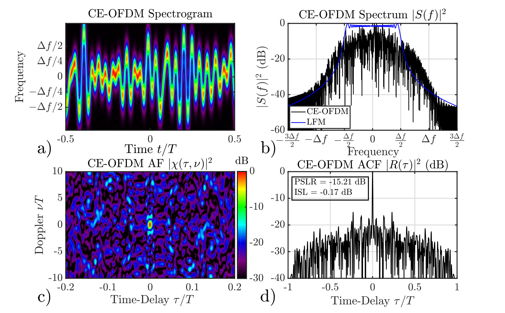
Figure 1 shows an example CE-OFDM waveform’s spectrogram, spectrum, AF, and ACF. The waveform is composed of sub-carriers that employ PSK symbols with generated from a pseudo-random sequence as described in [11]. The modulation index is chosen to synthesize a waveform with the same RMS bandwidth [18] as that of a LFM waveform with a Time-Bandwidth Product (TBP) of 200 which can be calculated in closed form as [13]
| (9) |
As explained earlier, the CE-OFDM waveform’s frequency modulation function is a finite Fourier series and is therefore an infinitely differentiable and smooth function. This smooth FM function is shown in panel (a) of Figure 1. As a result of the smooth FM function, the vast majority of the waveform’s energy is densely concentrated in a compact band of frequencies as is shown in panel (b) of Figure 1. As is described in [13], a CE-OFDM waveform utilizing PSK coding will essentially always produce a “Thumbtack-Like” AF shape. The sidelobe pedestal is clearly visible in the ACF of the waveform shown in panel (d). It is the goal of this paper to develope an algorithm that will further reduce the ACF sidelobe levels in a specified region of time-delays.
III The GD-GISL Algorithm
The first step in developing the GD-GISL algorithm is to discretize the waveform signal model and its design metrics. The CE-OFDM waveform’s instantaneous phase (2) can be transformed from the amplitude-phase Fourier series representation to the standard real-valued Fourier series as
| (10) |
The Fourier coefficients and lie on the unit circle such that and are derived from
| (11) | ||||
| (12) |
From here, (10) can be written as a linear sum using discrete variables as
| (13) |
where the phase values are grouped into a vector and the basis matrices and contain cosine and sine harmonics respectively such that the columns
| (14) | ||||
| (15) |
are sampled at some sampling rate which satisfies the Nyquist criterion.
From here, the development of the gradient-based GISL algorithm largely follows the description given in [12]. The GISL metric can be expressed in terms of the discretized ACF which is expressed as
| (16) |
where contains discretized samples of the ACF, is a discretized and zero-padded version of , and and are Discrete Fourier Transform (DFT) and Inverse DFT matrices respectively. The GISL metric is then expressed as the cost function [12]
| (17) |
where the vectors and are non-zero in the extent of the sidelobe and mainlobe regions respectively. In setting the cost function to the GISL metric, the optimization problem can be formally stated as
| (18) |
The GISL is an L-dimensional and highly non-convex objective function across the CE-OFDM parameter space on the order of in each dimension. Therefore, convergence to the global minimum is most certainly not guaranteed. Non-convex functions require a non-linear optimization routine, which is why here we expand upon the continuous nature of the CE-OFDM waveform and its modulation function to employ gradient-descent optimization. Gradient-descent is an iterative approach which takes some step in the direction of steepest descent
| (19) | ||||
| (20) |
where is the gradient operator. The gradient of (18), derived in the Appendix, is expressed as
| (21) |
where
| (22) |
Performing (19) and (20) iteratively until the Euclidean length of is below some threshold ensures that is very near a local minima. Alternatively, the routine may continue until it reaches a predetermined number of iterations .
We employ heavy-ball gradient-descent which includes weighted versions of the previous search-directions with the current gradient. This has been shown to converge quickly for these types of problems by dampening rapid transitions of the gradient thereby enforcing a smooth path to the minima. The search direction is altered by inclusion of previous gradients as
| (23) |
where . Since this method does not always ensure a descent, if in fact the current search direction is an ascent (i.e., the projection of the gradient onto the current search direction is positive), the current search direction is reset to the current gradient.
| (24) |
Once the search direction is established, a simple backtracking method is used to calculate the step size for the line search that satisfies sufficient decrease via the Armijo condition [19]. As mentioned earlier, to maintain continuity of the GISL gradient and to avoid diminishing returns thereafter, the parameter should take on values much lower than infinity but larger than roughly 6 [12]. These values for have been shown to consistently generate waveforms with a flat sidelobe response. On the other hand, letting results in waveforms whose ACFs possess more peaks and valleys, but overall less area in the specified sidelobe region . The steps of the GD-GISL algorithm are listed in Algorithm 1. Since the algorithm makes extensive use of FFTs in computing the GISL metric (21), it is substantially more computationally efficient compared to a brute-force numerical computation.
IV Several Illustrative Design Examples
This section demonstrates the GD-GISL algorithm using two waveform optimization design examples. Both examples optimize the GISL () of the waveform from Figure 1 over different sub-regions of the waveform’s ACF. The waveform time-series are sampled at a rate . The algorithm was set to run for a max number of iterations . Figure 2 shows the ACF, spectrum, and ACF zoomed in at the origin of the CE-OFDM waveform from Figure 1 and the resulting optimized CE-OFDM waveform whose ACF sidelobes were minimized over all time-delays excluding the mainlobe region. The initial waveform’s GISL for and PSLR values were -14.73 dB and -15.21 dB respectively. The optimized waveform’s GISL was -22.14 dB corresponding to a PSLR of -20.72 dB. It’s also important to note that the mainlobe width of the optimized waveform stayed the same width as its initial seed waveform. As explained in [13], the CE-OFDM’s RMS bandwidth, which controls the ACF mainlobe width, remains the same value for fixed and regardless of the PSK values . This precludes introducing constraints on RMS bandwidth to ensure the waveform’s ACF mainlobe width stays largely fixed as was done for a closely related waveform model in [20].
Figure 3 shows the result of optimizing the GISL of the CE-OFDM waveform from Figure 1 over a sub-region of time-delays . The initial waveform’s GISL and PSLR over this sub-region of time-delays was -16.8 dB and -17.51 dB respectively. The resulting optimized waveform’s GISL and PSLR values were -30.34 dB and -31.39 dB respectively, a substantial reduction of sidelobes in the specified region . Again, the optimized waveform’s mainlobe width stays fixed as does the waveform’s spectral extent.
One final important point is that the GD-GISL optimization routine assumes the CE-OFDM waveforms employ PSK with infinite granularity (i.e, ). Practical implementations of CE-OFDM waveforms will almost certainly employ a finite M-ary alphabet for the PSK symbols. Truncating these continuous symbols to an M-ary representation will introduce perturbations in the waveform’s instantaneous phase. These perturbations are likely to degrade the desirably low ACF sidelobes of the optimized waveform designs. This issue is illustrated in Figure 4 where the PSK symbols from the optimized waveform in Figure 3 is approximated by finite M-ary alphabets. As can be seen from the figure, as is reduced, the degree of perturbations in the PSK symbols is greater and the ACF sidelobes increase in the region of time-delays where the optimization routine was run on. There are two ways to mitigate this issue. The first is to utilize a large value to reduce the degree of perturbations in the implemented waveform. The second is to modify the GD-GISL algorithm to operate on finite M-ary alphabets. This approach may produce more favorable optimal designs with less perturbations than the waveforms shown in Figure 4. This will be a topic of future investigation.
V Conclusion
The GD-GISL minimization algorithm synthesizes CE-OFDM waveforms with low ACF sidelobes in a specified region of time-delays. The algorithm leverages methods developed in [12] which exploits FFTs in the majority of its operations making it computationally feasible to optimize CE-OFDM waveforms with a large number of sub-carriers . Results show that the algorithm is indeed capable of reducing CE-OFDM ACF sidelobes in a user-specified sub-region of time-delays while also maintaining the waveform’s ACF mainlobe width. Truncating these PSK symbols to M-ary alphabets introduces perturbations to the optimal design that results in increased ACF sidelobes. There are a number of avenues to pursue for future work. The first obvious one is to modify the algorithm to work with finite M-ary alphabets for PSK and other digital modulation techniques such as Quadrature Amplitude Modulation (QAM). The algorithm should also be generalizable to generating families of waveforms with desirable ACF and Cross-Correlation Function (CCF) properties such as the efforts of [16] and extendable to minimizing -norms on the AF of the waveform as well. Lastly, these optimization algorithms should also be applicable to the Multi-Tone Sinusoidal FM (MTSFM) waveform [20] of which the CE-OFDM waveform is a special case.
Appendix A Derivation of the Gradient of the GISL Metric
We define the cost metric as the GISL in (17) as
| (25) |
The Wirtinger definition of a complex derivative extended to vector calculus is [21]
| (26) |
where for an arbitrary transformation from a to a dimensional space,
| (27) |
is the Jacobian matrix.
We begin with the real to complex mapping from to
| (28) | ||||
where the matrix
| (29) |
results from the chain rule, and where places the elements of the operand along the diagonal of a square matrix such that the column is
| (30) |
Note that , , and are zero padded such that their dimensionality is now . Next, we map from to
| (31) | ||||
where the second term simplifies to 0 since and are considered independent variables. Next, mapping from to yields
| (32) | ||||
Then, since is a function of via (16),
| (33) | ||||
And, mapping from to
| (34) | ||||
And, since is directly a function of , we solve for by use of the quotient rule followed by chain rule
| (35) |
Finally, using (32)-(A) and inserting (31) into (28) produces the final result
| (36) |
where
| (37) |
Note that a function is said to be conjugate symmetric if and only if its Fourier transform is real valued [22]. Under the assumption that and are defined to be symmetric about 0 delay, then term exhibits conjugate symmetry since by definition, a waveform’s ACF is conjugate symmetric. Additionally, since we are applying a DFT matrix to a conjugate symmetric vector, the result is purely real and so the operator can be discarded.
References
- [1] S. C. Thompson, A. U. Ahmed, J. G. Proakis, J. R. Zeidler, and M. J. Geile, “Constant envelope ofdm,” IEEE Transactions on Communications, vol. 56, no. 8, pp. 1300–1312, 2008.
- [2] C.-D. Chung and S.-M. Cho, “Constant-envelope orthogonal frequency division multiplexing modulation,” in Fifth Asia-Pacific Conference on … and Fourth Optoelectronics and Communications Conference on Communications,, vol. 1, 1999, pp. 629–632 vol.1.
- [3] S. C. Thompson, Constant envelope OFDM phase modulation. University of California, San Diego, 2005.
- [4] E. M. N. Levanon, Radar Signals. Wiley-Interscience, 2004.
- [5] A. Aubry, V. Carotenuto, A. De Maio, A. Farina, and L. Pallotta, “Optimization theory-based radar waveform design for spectrally dense environments,” IEEE Aerospace and Electronic Systems Magazine, vol. 31, no. 12, pp. 14–25, 2016.
- [6] A. Hassanien, M. G. Amin, E. Aboutanios, and B. Himed, “Dual-function radar communication systems: A solution to the spectrum congestion problem,” IEEE Signal Processing Magazine, vol. 36, no. 5, pp. 115–126, 2019.
- [7] Q. Zhang, Y. Zhou, L. Zhang, Y. Gu, and J. Zhang, “Waveform design for a dual-function radar-communication system based on ce-ofdm-pm signal,” IET Radar, Sonar & Navigation, vol. 13, no. 4, pp. 566–572, 2019.
- [8] F. Gini, A. De Maio, and L. Patton, Waveform design and diversity for advanced radar systems. Institution of engineering and technology London, UK, 2012.
- [9] L. K. Patton and B. D. Rigling, “Autocorrelation and modulus constraints in radar waveform optimization,” in 2009 International Waveform Diversity and Design Conference, 2009, pp. 150–154.
- [10] R. Mohseni, A. Sheikhi, and M. A. M. Shirazi, “Constant envelope ofdm signals for radar applications,” in 2008 IEEE Radar Conference, 2008, pp. 1–5.
- [11] E. R. Biehl, C. A. Mohr, B. Ravenscroft, and S. D. Blunt, “Assessment of constant envelope ofdm as a class of random fm radar waveforms,” in 2020 IEEE Radar Conference (RadarConf20), 2020, pp. 1–6.
- [12] C. A. Mohr, P. M. McCormick, C. A. Topliff, S. D. Blunt, and J. M. Baden, “Gradient-based optimization of pcfm radar waveforms,” IEEE Transactions on Aerospace and Electronic Systems, vol. 57, no. 2, pp. 935–956, 2021.
- [13] D. G. Felton and D. A. Hague, “Characterizing the ambiguity function of constant-envelope ofdm waveforms,” 2023. [Online]. Available: https://arxiv.org/abs/2303.06009
- [14] J. P. Boyd, Chebyshev and Fourier spectral methods. Courier Corporation, 2001.
- [15] S. D. Blunt and E. L. Mokole, “Overview of radar waveform diversity,” IEEE Aerospace and Electronic Systems Magazine, vol. 31, no. 11, pp. 2–42, 2016.
- [16] E. Raei, M. Alaee-Kerahroodi, P. Babu, and M. R. B. Shankar, “Design of mimo radar waveforms based on lp-norm criteria,” 2021. [Online]. Available: https://arxiv.org/abs/2104.03303
- [17] J. Song, P. Babu, and D. P. Palomar, “Sequence design to minimize the weighted integrated and peak sidelobe levels,” IEEE Transactions on Signal Processing, vol. 64, no. 8, pp. 2051–2064, April 2016.
- [18] C. Cook and M. Bernfeld, Radar signals: an introduction to theory and application, ser. Electrical science series. Academic Press, 1967.
- [19] J. Nocedal and S. Wright, Numerical Optimization. Springer, 2006.
- [20] D. A. Hague, “Adaptive transmit waveform design using multitone sinusoidal frequency modulation,” IEEE Transactions on Aerospace and Electronic Systems, vol. 57, no. 2, pp. 1274–1287, 2021.
- [21] K. B. Petersen and M. S. Pedersen, “The matrix cookbook,” 2012.
- [22] J. Proakis and D. Manolakis, Digital Signal Processing: Principles, Algorithms, and Applications. Prentice-Hall International, 1996.