A diffuse interface approach for vector-valued PDEs on surfaces
Abstract
Approximating PDEs on surfaces by the diffuse interface approach allows us to use standard numerical tools to solve these problems. This makes it an attractive numerical approach. We extend this approach to vector-valued surface PDEs and explore their convergence properties. In contrast to the well-studied case of scalar-valued surface PDEs, the optimal order of convergence can only be achieved if certain relations between mesh size and interface width are fulfilled. This difference results from the increased coupling between the surface geometry and the PDE for vector-valued quantities defined on it.
1 Introduction
PDEs on surfaces remain an active field of research in applied mathematics and computational science. Due to their coupling with the geometry of such surfaces, PDEs are intrinsically nonlinear. This leads to new challenges in modeling and numerical analysis. Most of these challenges are addressed for scalar-valued surface PDEs, see [1] for a review. In the scalar case the coupling between surface geometry and the PDE is relatively weak, and thus numerical approaches established in flat spaces are applicable after small modifications. For vector-valued surface PDEs these approaches are no longer sufficient. Surface vector-fields often need to meet additional constraints. One example is the tangentiality of these fields. In this case, they need to be considered elements of the tangent bundle of the surface. This will lead to a strong nonlinear coupling between the surface geometry and the PDE. One break through which allows us to deal with these new challenges was the idea to express the solution and the surface differential operators in the global coordinate system of the embedding space and to penalize normal components, independently introduced in [2, 3, 4] and generalized in [5]. This approach essentially allows us to apply established tools for scalar-valued surface PDEs to each component. Popular approaches are surface finite elements (SFEM) and trace finite elements (TraceFEM), which have been applied to various problems in liquid crystal theory [2, 6, 7, 8, 9], fluid mechanics [10, 3, 11, 12, 13] and biological physics [14, 15, 16]. Numerical analysis results for these methods also exist, but are restricted to the most simple equations of this type, the surface vector-valued Laplace equation [17, 4], the surface vector-valued Helmholtz equation [18] and the surface Stokes equations [19, 20]. All these results show the necessity for an appropriate approximation of the geometric quantities that enter these equations. Optimal order of convergence can often only be achieved if this approximation is of a higher order than the solution. These results reflect the increased coupling between the surface geometry and the solution for vector-valued surface PDEs if compared with scalar-valued surface PDEs. This increase in complexity is also shown numerically by comparing scalar-, vector- and tensor-valued surface diffusion equations by various numerical methods [21].
Another popular method to solve surface PDEs, the diffuse interface method [22, 23] is less explored for vector-valued surface PDEs. Two examples, where solutions are compared with other more established methods are [2, 21]. The diffuse interface method approximates the surface PDE by a bulk PDE that can be solved with standard numerical tools. This makes the approach attractive to be used in various application areas for more complex problems, especially those where the surface evolves according to physical laws which depend on the vector-valued surface quantity. Such applications can be found in biology, e.g. in morphogenesis, where the method recently led to spectacular results [24]. However, knowing the subtleties associated with the approximation of geometric terms in SFEM and TraceFEM, discussed above, and the additional error emerging from the approximation of the diffuse interface method, such results should be considered with care.
We here consider a tangential vector-valued surface Helmholtz equations to explore the convergence properties of the diffuse interface methods. This can be considered as a model problem, and the obtained results can be assumed to be applicable also to other more complex surface PDEs. In Section 2 we introduce the surface model, review the described extension to the embedding space and required penalization of the normal component, which provides the basis for a SFEM discretization and derive from this the diffuse interface formulation. We formulate these approaches in variational form and provide a finite element (FEM) discretization. The diffuse interface approximation is justified by formal matched asymptotics, which directly follow from the results for scalar-valued surface PDEs [22]. In Section 3 we construct an analytical solution and perform various convergence studies. The results indicate the necessity for accurate approximations of the surface normals. These approximations can be obtained from the phase field variable or the signed distance function of the implicit surface description. Depending on the chosen approach specific minimal requirements regarding the relation of interface width and mesh size at the interface have to be meet for optimal convergence. Ignoring these requirements can result in numerical solution procedures that do not converge! These results significantly differ from the known results for the diffuse interface method for scalar-valued surface PDEs. In Section 4 we draw conclusions.
2 Model problem
We demonstrate the applicability of the diffuse interface approach by considering the surface vector-valued Helmholtz equation on a smooth, oriented two-dimensional surface without boundaries. The equation reads
| (1) |
for a tangential vector field defined in the tangent bundle of and a compatible right hand side . The considered differential operators and correspond to the metric-preserving covariant derivative . The diffuse interface formulation will be based on the SFEM formulation for vector-valued surface PDE’s, as detailed in [5]. The general idea is to express the solution and the operators in the global coordinate system of the embedding space and to penalize normal components. We denote the Euclidean coordinates of , by uppercase letters and consider Einstein’s sum convention. We consider the outward oriented normal , the surface identity and the shape operator . For we denote the formal extension to the embedding space by , for which we require . Finally we define the full tangential projection of such extended fields along all their components by , e. g. for a vector-valued field and for a 2-tensor-valued field .
Given these notations we can express the surface differential operators by their counterparts. Acting on the extended field this reads
| (2) | ||||
| (3) |
see [5] for details. To obtain the embedded variational formulation we use scalar products of pointwise full contraction of the tangential parts of the extended solution and the test function , e.g.
| (4) |
From these ingredients we set up a component wise solution-test space and write the embedded variational problem
| (5) | |||||
with an additional penalty term with prefactor to approximate . In this formulation each component can be considered by classical SFEM for scalar-valued fields, see [1].
Various numerical studies confirm the applicability of this approach. Numerical analysis provides various estimates of solution error convergence for surface mesh size . Here, we consider the surface to be approximated by faceted polyhedra . Such first order geometry approximation allows only linear Lagrangian elements for the discretization of the component solution-test space. This approach is referred to as the linear isogeometric ansatz. With the penalty prefactor one obtains quadratic convergence of the -error
Please note, by approximating by a faceted polyhedra we yield which significantly simplifies the discretized weak formulation of the Laplacian in eq. (5). Various numerical studies, also for more complicated problems [8, 14, 16], confirm quadratic order.
At first glance it seems straight forward to apply the tools introduced in [22] to each component in eq. (5) to obtain a diffuse interface approximation which turns the problem defined on into a problem defined in . However, eq. (5) contains various geometric terms, which are not considered in [22] or any subsequent analysis. The sensitivity of the solution to the approximation of these geometric terms is known from [4, 18] and contrary to the scalar case [25], higher order approximations for the surface and the solution only lead to better convergence properties if a higher order approximation of the normals is used in the introduced penalization term. So, the question arises if an additional approximation of the normals, resulting from an implicit description of the surface in the diffuse interface formulation, is sufficient to obtain the same convergence properties as the SFEM approach. We will answer this question in the following.
In order to formulate the diffuse interface approximation we extend the quantities , , and to the embedding space. We consider this component wise constant in the normal direction and denote the extended quantities by , , and , respectively. With this we can write , and . We now follow [22] and embed the surface in a bulk domain and use an implicit description of . For this purpose we use a signed distance function with and and a phase field function with interface width and . With these functions we can evaluate extended normals. We obtain
| (6) |
The surface delta function is approximated by , the classical double-well potential in Ginzburg-Landau energies [26]. Within this notation we substantiate the previously used constant normal extension by the closest point projection , e. g. , which is well defined for sufficient small such that . With this notation we express the surface scalar product by a scalar product of the embedding space
| (7) |
We use this embedded scalar product to set up the embedded variational problem with a component wise solution space . So the diffuse interface approximation of the component wise embedded variational problem eq. (5) reads
| (8) | ||||
Considering such component wise formulation as a coupled system of scalar fields, the matched asymptotic analysis of [22] provides formal convergence of eq. (2) to eq. (5) for . This establishes eq. (2) to be a diffuse interface approximation of eq. (1). Using this procedure any surface PDE can be reformulated into the corresponding diffuse interface approximation.
In analogy to the SFEM approach, we use a linear ansatz for the implicit geometric description by for a tetrahedral mesh of , where denotes the bulk mesh size in the interface . Within such ansatz the recovered surface or is a faceted polyhedra. The same ansatz is considered for the solution . This allows us to consider across the interface and we obtain
| (9) |
with the Helmholtz operator , the normal penalty term , a bulk stabilization and the right hand side , defined by:
respectively. Here we have used a component wise constant regularization outside the interface of as discussed for the scalar case in [22]. Inspired by the normal penalty condition, specified in [18] for the isogeometic case, we consider also within the diffuse interface approximation .
3 Results
We are interested in the convergence properties of the diffuse interface approach. We have to take into consideration that error measures will depend on and . For further discussion we define a relation to essentially express the number of mesh points across the interface for a given interface width. For our considerations we follow [27] and group those relations as linear, where so the number of points remains constant within the interface for , and higher order relations, where such that the number of points within the interface increases for , see Figure-1-[B].
Within the same setting, a linear ansatz for the geometric description and a linear ansatz for the solution, in [22] a numerical study was performed to estimate convergence rates. For a linear relation quadratic convergence was obtained for the scalar-valued problem, which can be considered optimal. It thus provides an upper limit to our vector-valued problem. However, it remains open if this limit can be reached in typical applications, where the signed distance function or the phase field variable need to be constructed from a surface mesh or where the phase field variable might be a solution to another PDE. In these cases the computation of the normals by eq. (6)[A] or [B] adds an additional source of error.
3.1 Benchmark formulation
To assess the impact of the major sources of approximations in the diffuse interface approach we perform a series of numerical experiments on a torus with radi and . The torus is embedded in . The analytical signed distance function for this geometry is given in by
| (10) |
The analytic phase field function is defined as before and for the analytic normal to we consider . On we consider the solenoidal tangential vector field and its extension to by , see Figure-1-[C]. This vector field will be used as an analytical solution for estimating the rate of error convergence. A compatible right hand side in eq. (9) is constructed by
| (11) |
To obtain results, which are comparable to the SFEM results in [18] we estimate and approximate surface error measured by the following diffuse interface error measures.
| (12) | ||||
| (13) |
For the subsequent numerical experiments we consider a set of mesh sizes , corresponding to bisections of . For each and relation we evaluate an associated and construct an adaptive tetrahedral mesh with meshsize in the diffuse interface of width . Off the interface, the mesh is only refined to preserve conformity. See Figure 1-[A]. We use the toolbox [28] to generate these meshes and evaluate . uses a triangulated surface as input which we generate via [29, 30] with vertices on and meshsize . Different methods exist to compute signed distance functions, see e.g. [31, 32, 33, 34, 35]. In a second order method is implemented. We use the finite element toolbox AMDiS [36, 37] to solve eq. (9), which uses an unpreconditioned BiCGstabL solver provided by PETSc [38] for the linear system.

3.2 Numeric evaluation of diffuse interface variables and normals
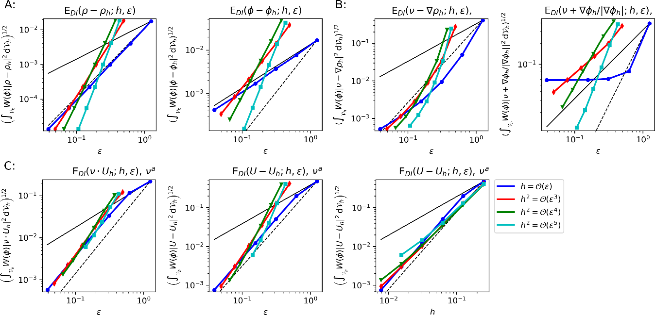
First we examine the convergence of errors in the chosen method to compute diffuse interface variables and derived from these fields. We compute and with for all and relations. We evaluate the diffuse interface -errors w.r.t. the analytical results , and and plot these quantities versus , see Figure-2-[A]. We observe the errors in evaluating converge quadratic, w.r.t. for linear relation. Higher order relations increase the rate of convergence. For we observe the rates of convergence to be reduced about one order compared to rates for . Recalling that while near the interface such reduced order of convergence is expected. Using the evaluated diffuse interface fields to determine the normals along the approaches described in eq. (6) we evaluate the diffuse interface -errors, and , see Figure-2-[B]. Using the linear relation, see Figure-2-[B](blue lines), we yield quadratic rate of convergence in while does not converge for . Considering higher order relations the convergence rates, w.r.t. , for could be improved beyond quadratic rate. In the case of a linear convergence rate could be achieved for and a quadratic rate is achieved with relation. We conclude that, in order to obtain normals with converging errors for , provides sufficient good approximations for to evaluate even for a linear relation. Yet considering the approach of computing normals from , we have to keep in mind that the rate of convergence, w.r.t. , is effectively reduced by two orders. Therefore, errors in normals only converge with higher order relations.
3.3 Error convergence for solution with analytic diffuse interface variables
Next we consider the analytical forms for , and and solve eq. (9) for a set of and relations. We evaluate the diffuse interface -error , see Figure-2-[C]. We observe that for a linear relation a quadratic rate of error convergence w.r.t. . This confirms the result from [22] for scalar-valued PDEs. Again, using higher order relations improves the rate of error convergence w.r.t. . But reviewing the error convergence w.r.t. it becomes apparent that is the crucial factor in convergence of and using higher order relations does not improve the rate of convergence for . So, we conclude that an analytical diffuse interface approximation does not impair the convergence of errors w.r.t. , and we observe a quadratic rate of convergence for linear relation.
3.4 Error convergence for diffuse interface approximation
We now combine both, consider approximations of the diffuse interface variables and obtained with and solve eq. (9) for a set of and relations. For these numeric solutions we evaluate the diffuse interface -error and the normal component , see Figure-3. For the normal approximation by , see Figure 3-[A] and a linear relation we observe quadratic rate of convergence for in the normal component and for the solution error. Due to the linear nature of the relation this behavior translates into quadratic rate of convergence w.r.t. with absolute values very close to the results with analytic diffuse interface variables and normals in Figure 2-[C]. For higher order relations the errors and convergence rates are also very close to the results with analytic diffuse interface variables and normals. Quite contrary, we observe while using the approximation of the errors in normal approximation to be dominant. Reviewing Figure 2-[B](right) we observe that the reduced normal approximation quality of this approach yields reduced convergence rate for controlling the solutions normal component, see Figure 3-[B](left) directly impacting the solution error convergence rate in Figure 3-[B](middle). In the case of a linear relation we observe no convergence in solution error, at we obtain a linear rate of convergence and for and we yield close to quadratic rates of convergence. Comparing to the results for analytic diffuse interface variables and normals we observe only for similar errors and rates of convergence for and w.r.t. and . Therefore, we conclude that the diffuse interface method, based on component-wise FEM, yields rates of error convergence compatible to the results of SFEM for vector-valued surface PDEs only if a high-quality signed-distance function is used to compute the normals. In this case a linear relation is sufficient. Alternatively if the normals are approximated by a relation with is required to achieve quadratic rate of convergence. A linear relation does not lead to convergence in this case! This significantly differs from the diffuse interface method for scalar-valued surface PDEs introduced in [22].

4 Discussion and conclusion
We provided a systematic derivation of a diffuse interface method to solve vector-valued surface PDEs. This approach builds on established SFEM formulations [5] and allows us to consider each component as a scalar quantity. The resulting system of equations can be solved by standard FEM. The connection to the surface PDE is established by formal matched asymptotic following [22] and is applicable to any vector-valued surface PDE. Along the same lines the approach can also be extended to tensor-valued surface PDEs.
Our numerical studies show that the same convergence properties as for SFEM can be achieved. With a linear isogeometric approach, which in our approach corresponds to linear Lagrange elements and a simplicial mesh, a quadratic order of convergence can be obtained for the considered vector-valued surface Helmholtz equation on a torus. However, to achieve this optimal order requires an accurate approximation of the surface normals. If they have to be numerically constructed a specific relation is necessary. If the computation of the normals is based on the signed distance function a linear relation is sufficient. However, if the computation of the normals is based on the phase field variable a linear relation does not lead to convergence and a higher order relation is required. The numerical results suggest to obtain a quadratic rate of convergence.
This result has severe consequences for applications. While for stationary surfaces, the computation of a signed distance function is not an issue and in such cases the diffuse interface method with normals computed from the signed distance function provides a valuable tool with optimal order of convergence, for moving surfaces this is no longer an option. The increased computational cost resulting from the computation of a signed distance function in each time step makes the approach inefficient. Assuming that the evolution of the surface is governed by a phase field problem which determines in each time step, the normals should be computed using . Such approaches are common for scalar-valued surface quantities, such as concentration [39, 40, 41, 42, 43, 44] or particle density [45, 46, 47]. However, for vector-valued surface quantities using this approach does not lead to convergence if a linear relation is considered. We can only expect convergence for higher order relations and quadratic convergence for . This needs to be respected in applications. Accounting for this issue increases the computational cost. However, the advantages of using basic numerical tools like linear Lagrangian elements and generic iterative solvers and the possibility to deal with topological changes in the evolution of the surface remain. This together with the possibility to couple the surface PDE with equations in the embedding space [48, 49], e.g. in two-phase flow problems with fluidic surfaces [50], makes this approach appealing for various applications.
Acknowledgments: This work was supported by the German Research Foundation (DFG) through grant VO 899/22 within the Research Unit ”Vector- and Tensor-Valued Surface PDEs” (FOR 3013). We further acknowledge computing resources provided by ZIH at TU Dresden and by JSC at FZ Jülich, within projects WIR and PFAMDIS, respectively.
References
- [1] G. Dziuk, C. M. Elliott, Finite element methods for surface PDEs, Acta Numerica 22 (2013) 289–396.
- [2] M. Nestler, I. Nitschke, S. Praetorius, A. Voigt, Orientational order on surfaces: The coupling of topology, geometry, and dynamics, Journal of Nonlinear Science 28 (2018) 147–191.
- [3] T. Jankuhn, M. A. Olshanskii, A. Reusken, Incompressible fluid problems on embedded surfaces: Modeling and variational formulations, Interfaces and Free Boundaries 20 (2018) 353–377. doi:{10.4171/IFB/405}.
- [4] P. Hansbo, M. G. Larson, K. Larsson, Analysis of finite element methods for vector laplacians on surfaces, IMA Journal of Numerical Analysis 40 (2020) 1652–1701.
- [5] M. Nestler, I. Nitschke, A. Voigt, A finite element approach for vector-and tensor-valued surface pdes, Journal of Computational Physics 389 (2019) 48–61.
- [6] I. Nitschke, M. Nestler, S. Praetorius, H. Löwen, A. Voigt, Nematic liquid crystals on curved surfaces: a thin film limit, Proceedings of the Royal Society A 474 (2214) (2018) 20170686.
- [7] I. Nitschke, S. Reuther, A. Voigt, Hydrodynamic interactions in polar liquid crystals on evolving surfaces, Phys. Rev. Fluids 4 (2019) 044002. doi:10.1103/PhysRevFluids.4.044002.
- [8] I. Nitschke, S. Reuther, A. Voigt, Liquid crystals on deformable surfaces, Proceedings of the Royal Society A 476 (2020) 20200313.
- [9] M. Nestler, I. Nitschke, H. Löwen, A. Voigt, Properties of surface Landau–de Gennes Q-tensor models, Soft Matter 16 (2020) 4032–4042.
- [10] S. Reuther, A. Voigt, Solving the incompressible surface Navier-Stokes equation by surface finite elements, Physics of Fluids 30 (2018) 012107. doi:10.1063/1.5005142.
- [11] S. Reuther, I. Nitschke, A. Voigt, A numerical approach for fluid deformable surfaces, Journal of Fluid Mechanics 900 (2020) R8. doi:10.1017/jfm.2020.564.
- [12] M. A. Olshanskii, A. Quaini, A. Reusken, V. Yushutin, A finite element method for the surface stokes problem, SIAM Journal on Scientific Computing 40 (2018) A2492–A2518.
- [13] P. Brandner, T. Jankuhn, S. Praetorius, A. Reusken, A. Voigt, Finite element discretization methods for velocity-pressure and stream function formulations of surface stokes equations, SIAM Journal on Scientific Computing 44 (4) (2022) A1807–A1832.
- [14] M. Nestler, A. Voigt, Active nematodynamics on curved surfaces – the influence of geometric forces on motion patterns of topological defects, Communications in Computational Physics 31 (2022) 947–965. doi:10.4208/cicp.OA-2021-0206.
- [15] Z. Wang, M. C. Marchetti, F. Brauns, Patterning of morphogenetic anisotropy fields, arXiv:2212.12215 (2022).
- [16] E. Bachini, V. Krause, A. Voigt, The interplay of geometry and coarsening in multicomponent lipid vesicles under the influence of hydrodynamics, arXiv:2302.04028 (2023).
- [17] J. Grande, C. Lehrenfeld, A. Reusken, Analysis of a high-order trace finite element method for PDEs on level set surfaces, SIAM Journal on Numerical Analysis 56 (2018) 228–255.
- [18] H. Hardering, S. Praetorius, Tangential errors of tensor surface finite elements, IMA Journal of Numerical Analysis (2022) drac015doi:10.1093/imanum/drac015.
- [19] M. A. Olshanskii, A. Reusken, A. Zhiliakov, Inf-sup stability of the trace P2-P1 Taylor-Hood elements for surface PDEs, Mathematics of Computation 90 (2021) 1527–1555. doi:10.1090/mcom/3551.
- [20] T. Jankuhn, M. A. Olshanskii, A. Reusken, A. Zhiliakov, Error analysis of higher order trace finite element methods for the surface Stokes equation, Journal of Numerical Mathematics 29 (2021) 245–267. doi:10.1515/jnma-2020-0017.
- [21] E. Bachini, P. Brandner, T. Jankuhn, M. Nestler, S. Praetorius, A. Reusken, A. Voigt, Diffusion of tangential tensor fields: numerical issues and influence of geometric properties, arXiv:2205.12581 (2022).
- [22] A. Rätz, A. Voigt, PDE’s on surfaces—a diffuse interface approach, Communications in Mathematical Sciences 4 (2006) 575–590.
- [23] M. Burger, Finite element approximation of elliptic partial differential equations on implicit surfaces, Computing and Visualization in Science 12 (2009) 87–100.
- [24] L. A. Hoffmann, L. N. Carenza, J. Eckert, L. Giomi, Theory of defect-mediated morphogenesis, Science Advances 8 (2022) eabk2712.
- [25] A. Demlow, Higher-order finite element methods and pointwise error estimates for elliptic problems on surfaces, SIAM Journal on Numerical Analysis 47 (2009) 805–827. doi:10.1137/070708135.
- [26] J. W. Cahn, J. E. Hilliard, Free energy of a nonuniform system. I. Interfacial free energy, The Journal of Chemical Physics 28 (2) (1958) 258–267.
- [27] X. Feng, A. Prohl, Numerical analysis of the Allen-Cahn equation and approximation for mean curvature flows, Numerische Mathematik 94 (1) (2003) 33–65.
- [28] F. Stenger, https://gitlab.mn.tu-dresden.de/iwr/meshconv.
- [29] J. Ahrens, B. Geveci, C. Law, 36 - paraview: An end-user tool for large-data visualization, in: C. D. Hansen, C. R. Johnson (Eds.), Visualization Handbook, Butterworth-Heinemann, Burlington, 2005, pp. 717–731. doi:https://doi.org/10.1016/B978-012387582-2/50038-1.
- [30] U. Ayachit, The paraview guide: a parallel visualization application, Kitware, Inc., 2015.
- [31] M. Sussmann, P. Smereka, S. Osher, A level set approach for computing solutions to incompressible two-phase flow, J. Comput. Phys. 119 (1995) 146–159.
- [32] G. Russo, P. Smereka, A remark on computing distance functions, J. Comput. Phys. 163 (2000) 51–67.
- [33] F. Bornemann, C. Rasch, Finite-element discretization of static Hamilton-Jacobi equations based on a local variational principle, Comput. Vis. Sci. 9 (2006) 57–69.
- [34] B. Lee, J. Darbon, S. Osher, M. Kang, Revisiting the redistancing problem using the Hopf–Lax formula, Journal of Computational Physics 330 (2017) 268–281.
- [35] M. Royston, A. Pradhana, B. Lee, Y. T. Chow, W. Yin, J. Teran, S. Osher, Parallel redistancing using the Hopf–Lax formula, Journal of Computational Physics 365 (2018) 7–17.
- [36] S. Vey, A. Voigt, Amdis: adaptive multidimensional simulations, Computing and Visualization in Science 10 (2007) 57–67.
- [37] T. Witkowski, S. Ling, S. Praetorius, A. Voigt, Software concepts and numerical algorithms for a scalable adaptive parallel finite element method, Advances in Computational Mathematics 41 (2015) 1145–1177.
- [38] S. Balay, S. Abhyankar, M. F. Adams, S. Benson, J. Brown, P. Brune, K. Buschelman, E. Constantinescu, L. Dalcin, A. Dener, V. Eijkhout, W. D. Gropp, V. Hapla, T. Isaac, P. Jolivet, D. Karpeev, D. Kaushik, M. G. Knepley, F. Kong, S. Kruger, D. A. May, L. C. McInnes, R. T. Mills, L. Mitchell, T. Munson, J. E. Roman, K. Rupp, P. Sanan, J. Sarich, B. F. Smith, S. Zampini, H. Zhang, H. Zhang, J. Zhang, PETSc/TAO users manual, Tech. Rep. ANL-21/39 - Revision 3.17, Argonne National Laboratory (2022).
- [39] M. Burger, Surface diffusion including adatoms, Communications in Mathematical Sciences 4 (2006) 1–51.
- [40] A. Rätz, A. Voigt, A diffuse-interface approximation for surface diffusion including adatoms, Nonlinearity 20 (2006) 177.
- [41] J. S. Lowengrub, A. Rätz, A. Voigt, Phase-field modeling of the dynamics of multicomponent vesicles: Spinodal decomposition, coarsening, budding, and fission, Physical Review E 79 (2009) 031926.
- [42] K. E. Teigen, P. Song, J. Lowengrub, A. Voigt, A diffuse-interface method for two-phase flows with soluble surfactants, Journal of Computational Physics 230 (2011) 375–393.
- [43] W. Marth, A. Voigt, Signaling networks and cell motility: a computational approach using a phase field description, Journal of Mathematical Biology 69 (2014) 91–112.
- [44] P. Werner, M. Burger, F. Frank, H. Garcke, A diffuse interface model for cell blebbing including membrane-cortex coupling with linker dynamics, SIAM Journal on Applied Mathematics 82 (2022) 1091–1112. doi:10.1137/21M1433642.
- [45] S. Aland, A. Rätz, M. Röger, A. Voigt, Buckling instability of viral capsids—a continuum approach, Multiscale Modeling & Simulation 10 (2012) 82–110.
- [46] S. Aland, J. Lowengrub, A. Voigt, A continuum model of colloid-stabilized interfaces, Physics of Fluids 23 (6) (2011) 062103.
- [47] S. Aland, J. Lowengrub, A. Voigt, Particles at fluid-fluid interfaces: A new navier-stokes-cahn-hilliard surface- phase-field-crystal model, Phys. Rev. E 86 (2012) 046321. doi:10.1103/PhysRevE.86.046321.
- [48] X. Li, J. Lowengrub, A. Rätz, Voigt, Solving PDEs in complex geometries: a diffuse domain approach, Communications in Mathematical Sciences 7 (2009) 81–107.
- [49] K. E. Teigen, X. Li, J. Lowengrub, F. Wang, A. Voigt, A diffuse-interface approach for modeling transport, diffusion and adsorption/desorption of material quantities on a deformable interface, Communications in Mathematical Sciences 4 (2009) 1009–1037.
- [50] S. Reuther, A. Voigt, Incompressible two-phase flows with an inextensible Newtonian fluid interface, Journal of Computational Physics 322 (2016) 850–858.