Low Frequency (100 - 600 MHz) Searches with Axion Cavity Haloscopes
Abstract
We investigate reentrant and dielectric loaded cavities for the purpose of extending the range of axion cavity haloscopes to lower masses, below the range where the Axion Dark Matter eXperiment (ADMX) has already searched. Reentrant and dielectric loaded cavities were simulated numerically to calculate and optimize their form factors and quality factors. A prototype reentrant cavity was built and its measured properties were compared with the simulations. We estimate the sensitivity of axion dark matter searches using reentrant and dielectric loaded cavities inserted in the existing ADMX magnet at the University of Washington and a large magnet being installed at Fermilab.
pacs
95.35.+dI Introduction
Observations imply that a large fraction, of order 27%, of the energy density of the Universe is some unknown substance called ”dark matter”Bertone. Although we do not know the identity of the particles constituting dark matter, we know two essential properties: the dark matter particles must be collisionless and cold. Cold means that their primordial velocity dispersion is sufficiently small, less than about today, so that it may be set equal to zero as far as the formation of large scale structure and galactic halos is concerned. Collisionless means that the dark matter particles have, in first approximation, only gravitational interactions. Particles with the required properties are referred to as ‘cold dark matter’ (CDM). Axions produced in the early universe by the process of “vacuum realignment’ axdm have those properties Ipser. Axions were originally proposed to solve the strong CP problem of the Standard Model of elementary particles PQ; WW, i.e. the puzzle of why the strong interactions conserve the discrete symmetries of parity P and charge conjugation times parity CP even though the Standard Model as a whole violates those symmetries. Therefore, the axion has a double motivation: it solves the strong CP and the dark matter problems simultaneously.
The axion is the quasi-Nambu-Goldstone boson associated with the spontaneous breaking of the UPQ(1) quasi-symmetry that Peccei and Quinn postulated to solve the strong CP problem. Its properties depend mainly on a single unknown parameter , called the axion decay constant, of order the energy scale at which UPQ(1) is spontaneously broken KSVZ; DFSZ. The axion mass and all axion couplings are inversely proportional to . The axion mass is given by
| (1) |
The cold axion cosmological energy density is a decreasing function of increasing axion mass axdm. The axion mass for which the cold axion cosmological energy density equals that of dark matter is of order eV, corresponding to of order GeV, however with very large uncertainties axrev. A major source of uncertainty is whether cosmological inflation happens before or after the phase transition in which UPQ(1) is spontaneously broken. In the post-inflationary scenario, i.e. if the PQ phase transition occurs after inflation, the cold axion cosmological energy density has contributions from axion string and axion wall decay in addition to the well-known contribution from vacuum realignment. Axion masses larger than eV are favored in the post-inflationary scenario because of these extra contributions.
In the pre-inflationary scenario, i.e. if the PQ phase transition occurs before inflation, the cold axion cosmological energy density receives a contribution from vacuum realignment only. The vacuum realignment contribution is uncertain in the pre-inflationary scenario because it depends on the misalignment angle of the axion field with respect to the minimum of its effective potential, at the start of the QCD phase transition. As a fraction of the critical energy density for closing the universe, the cold axion energy density in the pre-inflationary scenario is of order axrev
| (2) |
Since is presumably a random number between and , having the same value everywhere in the visible universe because the axion field was homogenized during inflation SYPi, there is 10% probability that is reduced by a factor 100, a 1% probability that it is reduced by a factor , and so on. For this reason, axion masses less than eV are favored in the pre-inflationary scenario.
The PQ phase transition occurs at a temperature of order the axion decay constant GeV. The reheat temperature at the end of inflation cannot be larger than the scale of inflation and in many models it is of order or less than the Hubble rate during inflation Weinberg. The non-observation of tensor perturbations requires GeV Planck18 or, equivalently, GeV. So, there is limited room in parameter space for the post-infationary scenario. On the other hand nothing forbids and the reheat temperature from being very low compared to . So there appears to be a lot of parameter space for the pre-infationary scenario, suggesting that searches for axions with lower masses are well-motivated.
A number of methods have been proposed to search for axion dark matter by direct detection on Earth. The topic is reviewed in Ref. RMP. The cavity haloscope method axdet, the earliest method proposed, has obtained the best results so far. A cavity haloscope is an electromagnetic cavity permeated by a strong magnetic field and instrumented to detect small amounts of power inside the cavity. When one of the cavity’s resonant frequencies equals the axion mass in natural units, i.e. when where is the angular frequency of the resonant mode, a small amount of microwave power is deposited inside the cavity as a result of axion to photon conversion in the applied magnetic field. The relevant interaction is
| (3) |
where is the fine structure constant, , and are respectively the axion, electric and magnetic fields, and is a model-dependent factor of order one. In the Kim-Shifman-Vainsthein-Zakharov (KSVZ) model KSVZ , whereas in the Dine-Fischler-Srednicki-Zhitnitskii (DFSZ) model DFSZ. Figure 1 shows the constraints that have been obtained so far on the electromagnetic coupling strength appearing in Eq. (3), , as a function of the axion mass. Using the cavity haloscope method, the Axion Dark Matter eXperiment (ADMX) has achieved sufficient sensitivity to find dark mattter axions at the expected halo density and with DFSZ coupling, the weakest coupling of the two benchmark models mentioned Du; Braine; Bartram. So far, ADMX has searched in the 600 to 1050 MHz range. It plans to search at higher frequencies using multi-cavity arrays Jihee. In this paper we explore methods to search lower frequencies, from approximately 100 to 600 MHz.
One approach to lower frequency axion dark matter detection is to replace the cavity with an LC circuit SST; Kahn. As with a haloscope cavity, the LC circuit is placed in a magnetic field. When its resonant frequency equals the axion mass in natural units, the axion dark matter field drives a tiny current in the circuit. Haloscopes with LC circuits, instrumented with the highest signal to noise detectors available and placed in strong spatially extended magnetic fields, are expected to achieve the sensitivity required to detect axion dark matter on Earth. Several pilot projects have been carried out ABRA; SLIC; ABRA2 and larger detectors are being planned DMRadio. An LC circuit is conveniently tuned by a variable capacitance. However the capacitance cannot be made arbitrarily small because a circuit always has some parasitic capacitance. Parasitic capacitance limits the highest frequency at which a large LC circuit may resonate SST. For this reason, LC circuits large enough to be sensitive to axion dark matter are not expected to reach the 200 - 600 MHz frequency range which is our main focus.
Instead, the approach we investigate here is to lower the resonant frequency of the cavity haloscope. This can be done of course by scaling up the physical size of the cavity, which indeed works very well assuming the magnetic field region is enlarged accordingly. However there are obvious limits as to how large the cavity and magnetic field region can be made. We therefore explore methods to lower the resonant frequency of the cavity without enlarging it. One approach is to fill the cavity with dielectric material, causing its resonant frequency to decrease as 1/ where is the dielectric constant. The form factor , which gives the strength of the coupling of the cavity mode to the axion dark matter field and which is defined in Eq. (6) below, decreases unfortunately as so that where is frequency. A second approach is to modify the cavity so as to make it “reentrant”. Reentrant cavities are described in Section IIIA. Reentrant cavities for axion dark matter detection were proposed and dicussed in Refs. UWA1; UWA2, including the building and characterization of a prototype cavity. The form factor of a reentrant cavity also decreases qualitatively as . So it is not clear at the outset whether reentrant or dielectric loaded cavities are the better approach. The goal of this paper is to explore the two approaches systematically. In particular we consider several possible reentant cavity designs and optimize them to achieve the highest possible form and quality factors. Whether one approach is better than the other ultimately depends on considerations such as the cost of low-loss dielectric materials and the lowest frequency that one wishes to attain with a given cavity.
The outline of our paper is as follows. In Section II, we give a general description of cavity haloscopes to prepare for the discussions that follow. In Section III, we report on numerical simulations of reentrant cavities. We consider several designs and optimize them for axion dark matter detection. In Section IV, we report on the measured properties of a prototype reentrant cavity that we built to validate the results of the numerical simulations. In Section V we report on numerical simulations of dielectric loaded cavities, evaluating their form and quality factors. In Section VI, we estimate the sensitivity that can be achieved using dielectric loaded and reentrant cavities inserted in the existing ADMX magnet at the University of Washington in Seattle and in a larger magnet that will be installed at Fermilab. Section VII summarizes our conclusions.
II Cavity haloscopes
If axions constitute the dark matter halo of the Milky Way Galaxy, we are immersed in a pseudo-scalar field, the axion field, oscillating with angular frequency
| (4) |
where is the speed of halo axions with respect to us. The ratio of their rest mass energy to their energy spread, called the “quality factor” of galactic halo axions, is expected to be of order because the typical speed of halo dark matter is . Note however that cold flows of axion dark matter are expected Ipser2. Such flows may have velocity dispersion much less than and correspondingly larger quality factors.
Henceforth, unless stated otherwise, we adopt units in which = 1.
A cavity haloscope searches for dark matter axions on Earth by attempting to convert them to microwave photons in an electromagnetic cavity permeated by a strong magnetic field axdet. The relevant coupling is given in Eq. (3). When the resonant frequency of cavity mode equals the axion mass in natural units () and the quality factor of the axion signal is large compared to the loaded quality factor of the cavity in mode , the power deposited into the cavity by the conversion process is
| (5) |
where is the coupling strength appearing in Eq. (3), is the energy density of dark matter axions at the detector location, is the volume of the cavity, is a nominal magnetic field strength inside the cavity, and
| (6) |
Here, is the actual magnetic field inside the cavity, is the dielectric constant, and the is the amplitude of the oscillating electric field in mode . The form factor expresses the coupling strength of mode to galactic halo axions. Generally speaking, the cavity mode with the highest form factor is the lowest TM mode, with the longitudinal direction being that of the static magnetic field .
Equation (5) shows that the signal power is proportional to the loaded quality factor of the cavtity when the axion signal falls exactly in the middle of the cavity bandwidth . Off resonance, the RHS of Eq. (5) is multiplied by the Lorentzian response function characteristic of driven harmonic oscillators. Since the Lorentzian here has width , the higher the quality factor the more narrow the frequency range over which the detector is sensitive at a given time. The overall figure of merit of a detector RSI; RMP is the rate at which it can search in frequency space with a given signal to noise ratio . The search rate is given by
| (7) |
where is the system noise temperature for detecting the microwave photons from axion conversion. Equation (7) assumes that the cavity bandwidth is wider than the axion signal bandwidth () and that the loaded quality factor equals one third the unloaded quality factor. This latter condition maximizes the search rate for given unloaded quality factor RSI. Equation (7) shows that the search rate is proportional to . This is the quantity we wish to optimize. In practice, varies relatively little. So most of our focus is on optimizing .
Both the reentrant cavity and the dielectric loaded cavity have form factors that decrease approximately as frequency squared as their resonant frequency is lowered. For this reason, it is convenient when comparing designs to express their performance by the variable defined by
| (8) |
where is the resonant frequency of the lowest TM mode, is the form factor at that frequency, and and are the form factor and resonant frequency of the empty cavity in its TM010 mode. For the designs discussed here, the empty cavity is always a cylinder of length and radius , in which case and
| (9) |
To facilitate comparison between different designs, in Eq. (6) is always be taken to be the volume of the empty cavity, .
III Numerical simulations of reentrant cavities
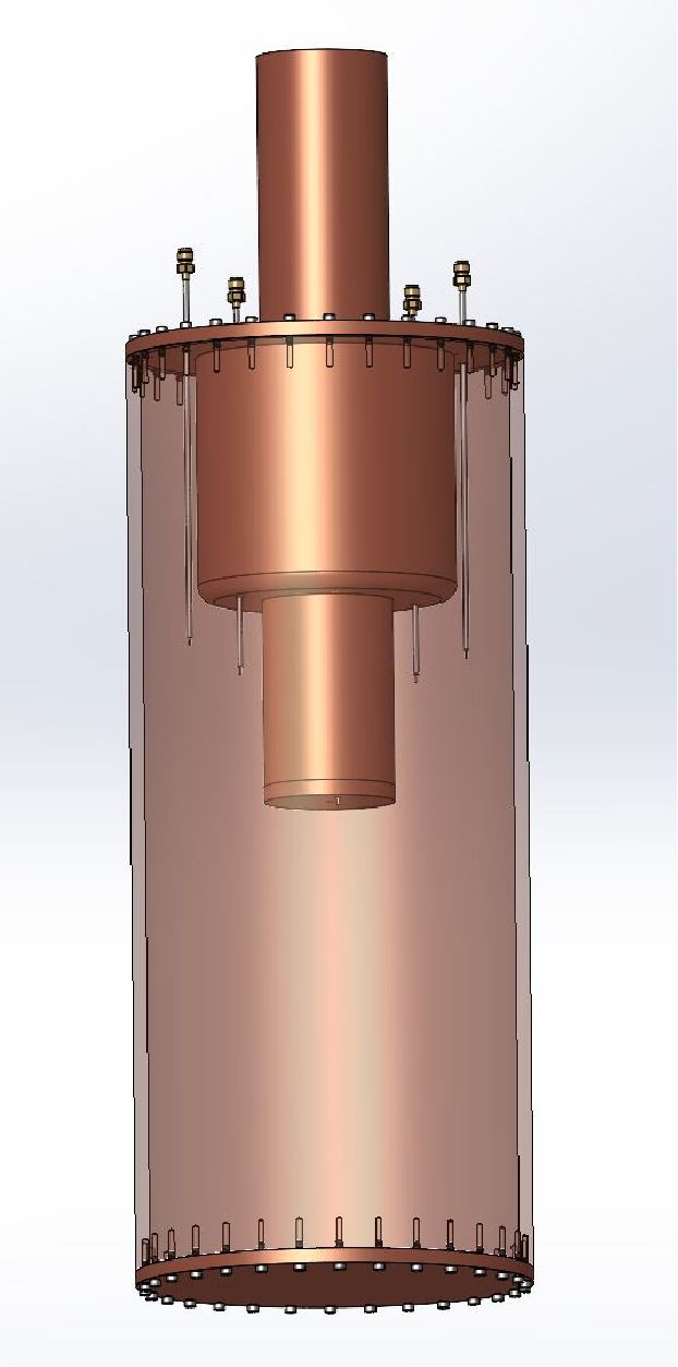
Figure 2 shows a tunable reentrant cavity consisting of a copper cylinder and a copper movable post that can be pushed in and out. The resonant frequency of the cavity decreases as the movable post is pushed in. All the reentrant cavity designs considered here are axially symmetric. The axial symmetry will be broken by the presence of the input and output ports that are necessary to couple out the axion signal and to characterize the cavity’s properties. In this paper, we ignore the perturbations that the input and output ports introduce.
In the limit of axial symmetry the reentrant cavity mode of interest for axion dark matter detection has magnetic and electric fields of the form:
| (10) |
where are cylindrical coordinates, and are the corresponding unit vectors. is in the direction both of the axis of axial symmetry of the cavity and of the static magnetic field . The mode with the largest form factor is the lowest frequency mode of the type given in Eqs. (10). It becomes the TM010 mode of the empty cylindrical cavity, when the post is removed.
In the remainder of this section, we report on reentrant cavity simulations aimed at identifying the design of the movable post(s) that yield the largest form factors and quality factors for axion dark matter searches.
III.1 Single movable post
Figure 2 shows a reentrant cavity tuned by a simple movable post. The figure defines the cavity length and radius , the radius and insertion depth of the movable post, and the rounding radius of the edge of the movable post’s end.
Figure 3 shows a map of the amplitude of the longitudinal component of the electric field in the lowest TM mode of a reentrant cavity. The form factor is proportional to the square of the volume integral of ; see Eq. (6). Figure 3 shows that the main contribution to comes from the region near the end of the post.
Figure 4 shows the resonant frequency as a function of the insertion depth of the movable post for the case = 1 m, = 0.2 m, = 0.1 m, and = 20 mm. The reentrant cavity in its lowest TM mode can be understood qualitatively as an LC circuit. The end of the movable post forms a capacitance with the bottom of the cavity. The oscillating current that charges and discharges this capacitance flows up (down) the post and down (up) the sides of the cavity. The circuit composed of the post and cavity sides has inductance. This inductance and the capacitance both increase as the post is inserted deeper, causing the resonant frequency to decrease. The resonant frequencies of the cavity TE modes do not change much as the post in inserted. There are no TEM modes. As a result the lowest TM mode does not cross any other modes. This is an advantage of the reentrant cavity approach since the frequency intervals where mode crossings occur require special treatment in axion cavity haloscope searches.
Figure 5(a) shows the form factor as a function of frequency for three different radii of the movable post. Qualitatively . Figure 5(b) displays the same information in terms of the factor defined in Eq. (8). The behavior shown is characteristic. By definition, goes to one as . Below , decreases quickly to a minimum of order 0.25 for and then increases again as is lowered further. The minimum value depends on the length of the cavity as discussed below. At the lowest frequencies, where the search is most challenging because the form factor is lowest, the best performance in is achieved by a post whose radius is about half the cavity radius.
Figure 6(a) shows the product of the quality factor times the skin depth as a function of frequency for several values of the movable post radius . The skin depth is assumed to be the same on all interior surfaces of the cavity. The quality factor is then equal to the product of 1/ times a factor which has dimension of lengh, is proportional to the overall size of the cavity and depends on its geometry. It is that factor which is plotted in the figure. The figure shows that the quality factor reaches a maximum when . Figure 6(b) shows as a function of frequency for several values of the movable post radius . may be considered a figure of merit for a particular geometry since the search rate is proportional to ; see Eq. (7). At the lowest frequencies, where the search is most challenging because the form factor is smallest, is largest when .
Figure 7 shows the dependence of and on the curvature radius by which the edge of the post endcap is rounded. The figure, which have a suppressed origin, shows that there is very little such dependence. It appears that rounding off the edge of the post’s endcap decreases both the form factor and the quality factor slightly in the case of a single post.
Figure 8 shows and when the cavity’s length is decreased, from 1.0 m to 0.55 m, while keeping fixed = 0.2 m, = 0.1 m and = 0.5 m. The figure shows that the product is nearly constant over the range shown. This is consistent with the fact that most of the contribution to the form factor comes from the region near the end of the movable post. In Fig. 3 the bottom third of the cavity is seen to contribute almost nothing to the form factor. It can therefore be removed without changing the sensitivity of the experiment. If we remove the bottom third, and are reduced by the factor 2/3, but is approximately constant, as and are multiplied by 3/2 approximately. The volume removed at no expense in sensitivity may be used for other purposes such as the placement of the mechanism that moves the tuning post. Alternatively, provided , the factor may be approximately doubled by installing a symmetrically placed post at the bottom of the cavity. In this case, to avoid mode localization in the bottom or top half of the caity, the two oppositely placed posts should be identical and have equal insertion depths.
In this subsection, we reported on simulations of a reentrant cavity of lenght = 1 m and radius = 0.2 m, because that is the volume available inside the bore of the ADMX magnet at the University of Washington in Seattle. However, the results are applicable to practically any cylindrical cavity by exploiting 1) the fact that the dependence of the dimensionless quantities and on the dimensionless variables , and is universal, and 2) the fact that is approximately constant as long as does not approach .
We sought ways to improve the performance of the reentrant cavity by modifying the design of the movable post. We found many modifications that made the performance worse. One modification that improves performance is to add to the first post a second concentric post with smaller radius. This is discussed in Subsection III.B. The performance can be improved still further by having a series of concentric posts with decreasing radii, as discussed in Subsection III.C. One example of a modification that decreases performance is to add a disk at the end of the movable post, as illustrated in Fig. 9. In all cases simulated, the addition of a disk decreased the form factor, regardless of the thickness and radius of the disk.
III.2 Fixed and movable posts
Figure 10 shows a reentrant cavity with a fixed post and a coaxial movable post that can slide through the fixed post. The figure defines the various dimensions of the posts, their lengths and , their radii and , and the radii and by which their ends are rounded. We simulated a cavity of length = 1 m and radius = 0.325 m. Such a cavity would fill the central volume of the Extended Frquency Range (EFR) magnet that the ADMX Collaboration plans to install and operate at Fermilab. The resonant frequency of the empty cavity in its lowest TM mode is = 353 MHz.
Our first step is to optimize the post dimensions so as to obtain the largest possible figure of merit at the lowest frequencies where we plan to operate, near 100 MHz. The optimization results do not depend sharply on the frequency where the optimization was done. The optimal values are = 0.176 m, = 0.19 m, = 70 mm, = 0.12 m and . The highest frequency that can be achieved is then 262 MHz, for . Higher frequencies, between 262 and 353 MHz, would be explored by using the cavity with a single post, as was described in the previous subsection.
Figure 11 shows the frequency of the optimized cavity as a function of the total insertion depth . We plot the relative frequency , where is the frequency of the empty cavity, versus to emphasize that the relationships between dimensionless quantities are quasi-universal. In the same spirit, Fig. 12 shows the dimensionless quantities and as a function of for the optimized cavity, with .
It is useful to state how these results can be used for a cavity with a different radius, e.g. = 0.2 m. Whatever the value of , the optimal values of the post dimensions are , , and , provided does not approach . If = 0.2 m and = 0.615 m, Figs. 11 and 12 for the optimized cavity apply without change. If instead = 0.2 m but = 1 m, Fig. 12 applies except that the values should be rescaled using the fact that = constant as long as does not approach . The comparison shows that the reentrant cavity with a fixed and a movable post performs somewhat better than the reentrant cavity with a simple movable post, improving the form factor typically by 10%. For example, at = 344 MHz, the reentrant cavity with = 0.2 m, = 1 m and a simple post of radius = 0.1 m, has = 0.235. The same cavity at the same frequency but with optimized fixed and movable posts has = 0.264.
III.3 Telescopic post
To explore how much the form factor of a reentrant cavity can be improved further by inserting a post with several segments of successively smaller radii, we simulated the cavity depicted in Fig. 13 for the case = 0.325 m and = 1.1 m. Figure 14 shows the amplitude of the longitudinal component of the elctric field in the lowest TM mode of such a cavity. In the simulation, the post segment with the smallest radius is inserted first, followed by the other segments in order of increasing radii. The parameters and , defined in Fig. 13, and the number of segments were varied to optimize and at low frequencies. Figures 15 shows the resulting factor and as a function of frequency for a cavity with , m and m. The simulations show that the telescopic post does improve the form factor at low frequencies, where the search is most challenging, compared to the fixed and movable posts setup. For example at 100 MHz, the frequency for which the fixed and movable posts were optimized, the telescopic post has whereas the fixed and movable posts setup has .
IV Prototype Reentrant Cavity
A prototype reentrant cavity with fixed and movable posts was built and tested at the University of Florida. Figure 16 shows a schematic drawing of the cavity. It was built of OFHC copper and tested at room temperature. Its dimensions are = 0.381 m, = 77 mm, = 0.102 m, = 54 mm, = 6 mm, = 27 mm and . Figure 17 shows our measurements of its resonant frequency as a function of total insertion depth and the prediction from the numerical simulations. The agreement here is very good.
Figure 18 shows the quality factor as a function of frequency and the prediction from the simulations. The measured values are 15% to 40% lower than predicted. This may be due in part to an increase in the skin depth, compared to that of pure copper, caused by lack of cleanliness of the cavity’s inner walls. However, even when a decrease in skin depth is allowed for, there is less than perfect agreement between theory and experiment in that Fig. 18 shows a dip in the measured values near 430 MHz whereas there is no such dip in the predicted values. We established that the dip is due to the mixing of the mode of interest, the cavity lowest TM mode, with a mode located outside the cavity. Indeed the dip can be made deeper and displaced in frequency by modifying the cavity environment. We believe the coupling between the interior and exterior of the cavity occurs through two small holes that were made in the endplate of the movable post. The holes were intended to allow input and output ports located there but, when the measurements were made, the two small holes were unused and left open. This issue will be investigated further.
V Numerical simulations of dielectric loaded cavities
In this section we investigate dielectric loading as a means to lower the resonant frequency of a cylindrical cavity in its lowest TM mode, keeping the cavity radius fixed. The cavity is tuned by moving a metallic rod sideways, a standard method used in cavity haloscopes. We assume that the dielectric material has properties similar to those of sapphire. Sapphire has a dielectric constant ranging from 9.3 to 11.5 depending on orientation and, for the purpose of cavity haloscopes, negligibly small dielectric losses at cryogenic temperatures Krupka. Alumina (Al2O3) has the same chemical composition as sapphire and similar dielectric constant, but is more economical. High purity alumina has adequate dielectric losses for the purpose of axion haloscopes. In Ref. Alford the measured is approximately at room temperature. In our simulations, and .
Figure 19 depicts cross-sectional views of two possible designs. The cavity in (a) has a large ceramic cylinder machined to allow the movement of the metallic tuning rod. The cavity in (b) has instead many ceramic rods of small radius. Using many small rods is obviously simpler and more feasible in terms of fabrication.
A cavity of radius = 0.325 m and length = 1 m was simulated in three configurations, with = 9, 26, and 61 dielectric rods, as shown in Fig. 20. In all cases, the dielectric rods have radius 12.5 mm, the metallic tuning rod has radius 56 mm for = 9, and 65 mm for = 26 and 61. The frequency range 165-370 MHz is covered without gaps by the three configurations. The cavity with a metallic tuning rod of radius 50 mm and no dielectric rods covers 370-525 MHz.
Figure 21 shows and as a function of frequency for the three dielectric loaded configuations. Unlike reentrant cavities, dielectric loaded cavities are prone to mode crossings. In this particular example, each configuration has one major mode crossing where the form factor dips.
VI Sensitivity estimates
In this section, we estimate the downward reach in frequency of reentrant and dielectric loaded cavities installed in the magnet presently in use by ADMX at the University of Wasington (UW) in Seattle and in the EFR magnet that ADMX plans to install and operate at Fermilab. For the UW magnet, we take = 1 m, = 0.2 m, and = 7.5 T. For the EFR magnet = 1 m, = 0.325 m, and = 9 T.
We make two alternative assumptions about the density and energy dispersion of the local dark matter axion density. Assumption A is that the axion energy density is = 450 MeV/cc and = . Assumption A is what the ADMX Collaboration has consistently used in the past to derive limits on the coupling from its observations. Assumption B is the prediction of the galactic halo model described in Ref. Duffy. Observational evidence is claimed for that model in Refs. Duffy; Chak. The model predicts the existence on Earth of a cold flow, called the ”Big Flow”, with energy density estimated to be not less than 6 GeV/cc Chak and velocity dipersion not more than 70 m/s Banik. This latter upper limit implies a quality factor for the axion signal from the Big Flow not less than . For assumption B, we set = 6 GeV/cc and = .
Combining Eqs. (5) and (7) we have
| (11) |
Since we ask how low in frequency a given detector may go with sufficient signal to noise ratio to find or rule out axions under stated conditions, we are interested in the frequency dependence on the RHS of Eq. (11). We assume that the search rate over a logarithmic frequency scale is fixed at some reasonable value, similar to what ADMX has achieved in the past. We assume that , a reasonable value for searches at the lowest envisaged frequencies in view of our simulations. Hence . We assume that the total noise temperature is dominated by the physical temperature of the cavity, in which case is frequency independent. This is discussed further in the next paragraph. Since , and in the anomalous skin depth regime appropriate for the cryogenic temperatures at which we plan to operate the cavity, we have
| (12) |
where we show explicitly those factors that depend on the magnet used (UW or EFR) and on the assumptions on the local axion dark matter density (A or B). Equation (12) shows that searches with reentrant or dielectric loaded cavities become sharply more challenging as the frequency is lowered, mainly because of the worsening form factor and the decreasing coupling. It is our goal to estimate the lowest frequency at which the search is feasible under stated conditions, with the understanding that the search is then comparatively easy at frequencies larger than of order .
The total noise temperature is the sum of the physical temperature of the cavity and the system noise temperature of the detector of microwave photons produced by axion to photon conversion. Our assumption is that is of order or less. At present the ADMX detector at UW achieves 150 mK using a dilution refrigerator. The so-called “quantum limit” on the noise temperature of receivers is = 29 mK . John Clake and collaborators Muck developed quantum limited SQUID detectors for ADMX axion searches in the 600-800 MHz range Aszt; Du. Our assumption regarding is satisifed if near quantum limited receivers are developed and used in the 100-600 MHz range.
When estimating the sensitivity under the various stated assumptions we use as a benchmark the ADMX search reported in Ref. Du. It excluded DFSZ coupled axions in the frequency range 645-678 MHz using the UW magnet under assumption A on the local axion density. The cavity was tuned upwards from the empty cavity resonant frequency = 574 MHz using a copper tuning rod. In that search 0.4 and 300 mK. The signal to noise ratio was approximately 4 because of the desirability of having of order one candidate signal per cavity tune from statistical fluctuations in the noise and the fact that the noise is Gaussian distributed for the medium frequency resolution appropriate in a search under assumption A.
VI.1 Using the UW magnet
Under assumption A (Maxwell-Boltzmann) and the above stated conditions, Eq. (12) implies
| (13) |
Since 4 is necessary under assumption A, the search is sensitive to a coupling of the axion to two photons
| (14) |
Although sensitivity to DFSZ coupling is lost, the search is still sensitive to KSVZ coupling over a wide frequency range. It is also sensitive to many models of dark matter in the form of axion-like particles, as well as to QCD axions in theories where the coupling to two photons is enhanced for cosmological reasons, such as axion initial kinetic misalignement axcog; Servant, or particle physics reasons such as in the photophilic hadronic axion model of ref. Ring.
Under assumption B (Big Flow), the RHS of Eq. (12) is multiplied by compared to the search under assumption A in view of the increases in and . Hence
| (15) |
On the other hand, a high resolution search that fully exploits assumption B requires 14 because the noise is exponentially distributed in such a search and there are of order frequency bins per cavity tune in which candidate signals may occur Hires. Hence the lowest frequency at which sensitivity to DFSZ coupling can be achieved under the stated conditions is
| (16) |
VI.2 Using the EFR magnet
Compared to the UW magnet is multipled by = 3.8. Moreover, is lowered to 574 MHz = 353 MHz. Under assumption A (Maxwell-Boltzmann), Eq. (14) is replaced by
| (17) |
The lowest frequency at which sensitivity to DFSZ coupling can be achieved under the stated conditions is then
| (18) |
Under assumption B (Big Flow), the RHS of Eq. (15) is multiplied by the factor 3.8 in addition to the replacement 574 MHz 353 MHz for the resonant frequency of the empty cavity. This yields
| (19) |
VII Summary
We argued that there is comparatively more room in parameter space for inflation to occur after the PQ phase transition than before that transition.. This motivates axion dark matter searches at frequencies lower than where ADMX has already searched. The resonant frequency of axion haloscopes can be lowered by increasing the overall size of the cavity. Although attractive in several respects, this approach is limited by the size of available magnets in which to insert the cavity. In this paper we explored instead the possibility of lowering the resonant frequency by making the cavity reentrant or by loading it with dielectric material.
We simulated reentrant and dieletric loaded cavities numerically to compute their form factors and quality factors. We explored several designs of the movable post, that is inserted in a reentrant cavity to tune it, and optimized the post dimensions. The tuning posts with the highest figure of merit have radii that decrease with depth into the cavity. Our results are presented in a way which can be easily applied to cylindrical cavities of arbitrary dimensions.
We built a tunable reentrant cavity and compared its measured properties with the simulations. The agreement was excellent in the plot of resonant frequency versus tuning post insertion depth. In the plot of the quality factor versus frequency, the measured values were between 15% to 40% lower than the predicted ones. The origin of this discrepancy is under further investigation.
For both the reentrant cavity and the dielectric loaded cavity the form factor decreases with decreasing frequency qualitatively as , so that an axion search becomes progessively more challenging as the frequency is lowered. We estimated the lowest frequency at which a search with DFSZ sensitivity can be carried out using the magnet presently used by ADMX at the University of Washington and the larger EFR magnet that ADMX plans to operate at Fermilab. The estimates are given by Eqs. (16), (18) and (19) for two alternative assumptions about the local dark matter density.
Acknowledgements.
This work was supported by the U.S. Department of Energy through Grants DE-SC0022148, DE-SC0009800, DESC0009723, DE-SC0010296, DE-SC0010280, DE-SC0011665, DEFG02-97ER41029, DEFG02-96ER40956, DEAC52-07NA27344, DEC03-76SF00098, and DESC0017987. Fermilab is a U.S. Department of Energy, Office of Science, HEP User Facility. Fermilab is managed byFermi Research Alliance, LLC (FRA), acting under Contract No.0 DE-AC02-07CH11359. Additional support was provided by the Heising-Simons Foundation and by the Lawrence Livermore National Laboratory and Pacific Northwest National Laboratory LDRD offices. LLNL Release No. LLNL-JRNL825283. UWA was funded by the ARC Centre of Excellence for Engineered Quantum Systems, CE170100009, and Dark Matter Particle Physics, CE200100008. Ben McAllister is funded by the Forrest Research Foundation. Chelsea Bartram acknowledges support from the Panofsky Fellowship at SLAC.References
- (1) See, for example, Particle Dark Matter, edited by G. Bertone, Cambridge Uivversity Press, 2010.
- (2) J. Preskill, M. Wise and F. Wilczek, Phys. Lett. B120 (1983) 127; L. Abbott and P. Sikivie, Phys. Lett. B120 (1983) 133; M. Dine and W. Fischler, Phys. Lett. B120 (1983) 137.
- (3) J. Ipser and P. Sikivie, Phys. Rev. Lett. 50 (1983) 925.
- (4) R. D. Peccei and H. Quinn, Phys. Rev. Lett. 38 (1977) 1440 and Phys.Rev. D16 (1977) 1791.
- (5) S. Weinberg, Phys. Rev. Lett. 40 (1978) 223; F. Wilczek, Phys. Rev. Lett. 40 (1978) 279.
- (6) J. Kim, Phys. Rev. Lett. 43 (1979) 103; M. A. Shifman, A. I. Vainshtein and V. I. Zakharov, Nucl. Phys. B166 (1980) 493.
- (7) M. Dine, W. Fischler and M. Srednicki, Phys. Lett. B104 (1981) 199; A. Zhitnitskii, Sov. J. Nucl. 31 (1980) 260.
- (8) Reviews of axion cosmology include: P. Sikivie, Lect. Notes Phys. 741 (2005) 083513; D.J.E. Marsh, Phys. Rep. 643 (2016) 1.
- (9) S.-Y. Pi, Phys. Rev. Lett. 52 (1984) 1725.
- (10) S. Weinberg, Cosmology, Oxford University Press, 2008.
- (11) Y. Akrami et al.(Planck Collaboration), Astron. and Astroph. 641 (2020) A10.
- (12) P. Sikivie, Rev. Mod. Phys. 93 (2021) 015004.
- (13) P. Sikivie, Phys. Rev. Lett. 51 (1983) 1415, [Erratum: Phys. Rev. Lett. 52 (1984) 695], and Phys. Rev. D32 (1985) 2988, [Erratum: Phys. Rev. D36 (1987) 974].
- (14) C. O’Hare, Axion Limits, July 2022, https://cajohare.github.io/AxionLimits/ .
- (15) N. Du et al., Phys. Rev. Lett. 120 (2018) 151301.
- (16) T. Braine et al., Phys. Rev. Lett. 124 (2020) 101303; C. Bartram et al., Phys. Rev. D103 (2021) 032002.
- (17) C. Bartram et al., Phys. Rev. Lett. 127 (2021) 261803.
- (18) J. Yang et al., Springer Proc. Phys. 245 (2020) 53.
- (19) P. Sikivie, N. Sullivan and D. Tanner, Phys. Rev. Lett. 112 (2014) 131301.
- (20) Y. Kahn, B.R. Safdi and J. Thaler, Phys. Rev. Lett. 117 (2016) 141801.
- (21) J.L. Ouellet et al., Phys. Rev. Lett. 122 (2019) 121801, and Phys. Rev. D99 (2019) 052012.
- (22) N. Crisosto et al., Phys. Rev. Lett. 124 (2020) 241101.
- (23) C.P. Salemi et al., Phys. Rev. Lett. 127 (2021) 081801.
- (24) L. Brouwer et al., arXiv:2204.13781, and A. AlShirawi et al., arXiv:2302.14084.
- (25) B.T. McAllister, S.R. Parker and M.E. Tobar, Phys. Rev. D94 (2016) 042001.
- (26) B.T. McAllister et al., J. Appl. Phys. 122 (2017) 144501
- (27) P. Sikivie and J.R. Ipser, Phys, Lett. B291 (1992) 288.
- (28) C. Hagmann, P. Sikivie, N. Sullivan, D.B. Tanner and S.-I. Cho, Rev. Sci. Ins. 61 (1990) 1076.
- (29) J. Krupka et al., Meas. Sci. Technol. 10 (1999) 387.
- (30) N.M. Alford and S.J. Penn, J. Appl. Phys. 80 (1996) 5895.
- (31) L.D. Duffy and P. Sikivie, Phys. Rev. D78 (2008) 063508.
- (32) S.S. Chakrabarty, Y. Han, A.H. Gonzalez and P. Sikivie, Phys. Dark Univ. 33(2021) 100838.
- (33) N. Banik and P. Sikivie, Phys. Rev. D93 (2016) 103509.
- (34) M. Mück et al., Appl. Phys. Lett. 72 (1998) 2885.
- (35) S.J. Asztalos et al., Phys. Rev. Lett. 104 (2010) 041301.
- (36) R.T. Co, L.J. Hall and K. Harigaya, Phys. Rev. Lett. 120 (2018) 211602, and Phys. Rev. Lett. 124 (2020) 251802;
- (37) C. Eroncel et al., JCAP et al. 10 (2022) 053.
- (38) A.V Sokolev and A. Ringwald, JHEP 06 (2021) 123.
- (39) L.D. Duffy et al., Phys. Rev. Lett. 95 (2005) 091304; L.D. Duffy et al., Phys. Rev. D74 (2006) 012006; J. Hoskins et al., Phys. Rev. D84 (2011) 121302.