Entanglement and localization in long-range quadratic LindbladiansPreprint: APS/123-QEDPreprint: APS/123-QED

Alejandro Cros Carrillo de Albornoz Affiliation: Department of Physics and Astronomy, University College London, Gower Street, London WC1E 6BT, United Kingdom Dominic C. Rose Affiliation: Department of Physics and Astronomy, University College London, Gower Street, London WC1E 6BT, United Kingdom Arijeet Pal Affiliation: Department of Physics and Astronomy, University College London, Gower Street, London WC1E 6BT, United Kingdom Affiliation: Department of Physics and Astronomy, University College London, Gower Street, London WC1E 6BT, United Kingdom Affiliation: Department of Physics and Astronomy, University College London, Gower Street, London WC1E 6BT, United Kingdom Affiliation: Department of Physics and Astronomy, University College London, Gower Street, London WC1E 6BT, United Kingdom

August 11, 2026

Abstract

Existence of Anderson localization is considered a manifestation of coherence of classical and quantum waves in disordered systems. Signatures of localization have been observed in condensed matter and cold atomic systems where the coupling to the environment can be significantly suppressed but not eliminated. In this work we explore the phenomena of localization in random Lindbladian dynamics describing open quantum systems. We propose a model of one-dimensional chain of non-interacting, spinless fermions coupled to a local ensemble of baths. The jump operator mediating the interaction with the bath linked to each site has a power-law tail with an exponent $p$ . We show that the steady state of the system undergoes a localization entanglement phase transition by tuning $p$ which remains stable in the presence of coherent hopping. Unlike the entanglement transition in the quantum trajectories of open systems, this transition is exhibited by the averaged steady state density matrix of the Lindbladian. The steady state in the localized phase is characterized by a heterogeneity in local population imbalance, while the jump operators exhibit a constant participation ratio of the sites they affect. Our work provides a novel realization of localization physics in open quantum systems.

Introduction.— The interplay of coherence and disorder in quantum systems leads to the existence of the phenomena of localization Evers and Mirlin 2008, shown to remain stable in the presence of many-body interactions Basko et al. 2006; Gornyi et al. 2005; Pal and Huse 2010; Oganesyan and Huse 2007; Nandkishore and Huse 2015; Abanin et al. 2019. Such localized systems protect coherence and provide a route to stabilizing quantum phases of matter out of equilibrium Huse et al. 2013; Bahri et al. 2015; Parameswaran and Vasseur 2018. Even though localization is stable in isolated quantum systems, the presence of interactions with a bath can destroy the coherence Levi et al. 2016; Medvedyeva et al. 2016; Lüschen et al. 2017; Lenarčič et al. 2018; Lunt and Pal 2020; Lenarčič et al. 2020; Wybo et al. 2020; Hamazaki et al. 2022; Kawabata et al. 2022; García-García et al. 2022; Szyniszewski et al. 2022; Mák et al. 2023. In particular, the role of baths in destabilizing many-body localization resulting in a thermal steady state is of fundamental importance Sels 2022; Morningstar et al. 2022. Interaction with baths are unavoidable for experiments probing late time behavior, and a theoretical understanding is required for the interpretation of the observations Lüschen et al. 2017; Fitzpatrick et al. 2017; Li et al. 2019a; Mi et al. 2022

Open quantum systems (OQS) can host steady states which are manifestly out of equilibrium and protect coherence from environmental noise, such as decoherence free subspaces Zanardi 1997; Zanardi and Rasetti 1997; Lidar et al. 1998 and noiseless subsystems Knill et al. 2000; Zanardi 2000, among other non-equilibrium phenomena Albert et al. 2016; Landi et al. 2021; Sieberer et al. 2016; Maghrebi and Gorshkov 2016; Torre et al. 2013. The long time dynamics leading up to the stationary state have also been shown to present complex metastable behavior Macieszczak et al. 2016; Rose et al. 2016; Macieszczak et al. 2021; Rose et al. 2022, while periodic driving can enable time crystalline phenomena Iemini et al. 2018; Zhu et al. 2019; Gambetta et al. 2019; Riera-Campeny et al. 2020; O’Sullivan et al. 2020; Keßler et al. 2021; Passarelli et al. 2022a; Buča et al. 2019. Quantum trajectories of OQS, providing individual stochastic realizations of the systems pure-state evolution, can exhibit non-trivial trajectories statistics that cannot be detected in either the averaged time-evolution of the density matrix or its steady state Garrahan and Lesanovsky 2010; Carollo et al. 2018; Carollo et al. 2019; Carollo and Pérez-Espigares 2020; Carollo et al. 2021; Olmos et al. 2012; Olmos et al. 2014; Lesanovsky et al. 2013; Marcantoni et al. 2021; Hickey et al. 2012. In particular, recent work demonstrating entanglement transitions in quantum trajectory ensembles has spurred interest for quantum information processing Li et al. 2019b; Skinner et al. 2019; Li et al. 2018. Altogether, the preservation of coherence in non-equilibrium OQS suggests that it may also be possible for localized behavior to survive in the presence of dissipation.

Refer to caption — Figure 1: (a) Schematic figure of the model: The spatial power-law profile of each jump operator, given by exponent $p$ , for the heterogeneous baths shows the coupling to a system of spinless fermions hopping in a 1D lattice. We consider the mutual information between fermions in region A and B ( $\mathcal{I}$ ). (b) Disorder averaged mutual information between $A$ and $B$ in the steady state ( $\overline{\mathcal{I}}_{\infty}$ ) as a function of system size $L$ , with $L_{A}=L_{B}=L_{C}=L/3$ For each value of $p$ (shown in the legend) the curves are fitted to the form $\ln(\overline{\mathcal{I}}_{\infty})=\Delta\ln(L)+c$ . The fitting parameter $\Delta$ is shown in the legend. (c) $\overline{\mathcal{I}}_{\infty}$ between $A$ and $B$ in the steady state as a function of subsystem size $L_{A}$ with total system size $L=10^{3}$ . $L_{C}$ is fixed at $L/3$ . Curves were fitted according to $\overline{\mathcal{I}}_{\infty}=a(L_{A})^{c}+b\log(L_{A})$ . Note $c\approx 1/2$ for all $p$ . For both (b), (c): Curves are color-coded to a given $p$ according to the legend in panel (b). Error bars are not visible. Details on disorder realizations are included in SM7.

Quadratic Lindbladians have emerged as a testbed for studying various concepts in OQS Prosen 2008; Prosen and Pižorn 2008; Guo and Poletti 2017; Prosen 2010; Mahajan et al. 2016; Zanoci and Swingle 2016; Lieu et al. 2020; Barthel and Zhang 2022; D’Abbruzzo et al. 2022; Costa et al. 2022; Vernier 2020, due to simplifications enabled by their non-interacting nature. In this article we propose and investigate the properties of a quadratic fermionic model of localization induced by coupling to an heterogeneous bath, where the local degrees of freedom couple to randomly varying baths in space, similar to recent work on random Lindbladians Denisov et al. 2019; Can et al. 2019; Can 2019; Sá et al. 2020; Sá et al. 2020; Wang et al. 2020; Sommer et al. 2021; Tarnowski et al. 2021; Lange and Timm 2021; Li et al. 2022; Orgad et al. 2022. The baths are modeled using a Lindbladian formalism for OQS where the jump operators couple distant sites, realizable in the collective dissipation of atomic arrays Yamamoto et al. 2016; Marino 2022; Seetharam et al. 2022; Norcia et al. 2018; Miranda et al. 2017; Needham et al. 2019; Jones et al. 2018; Wang and Fazio 2021. The locality of the jump operators mediating the interaction via the bath is a tunable parameter, driving a phase transition between localized and delocalized steady states, the strength of the couplings decaying as a power-law in separation between sites in the localized phase. The steady state properties closely relate to the single-particle localization transition of power-law banded matrices for purely unitary dynamics Fyodorov and Mirlin 1991; Mirlin et al. 1996; Casati et al. 1990; Casati et al. 1993; Schenker 2009; Bourgade 2018; Varga 2002; Cao et al. 2017. Furthermore, we studied the effect of introducing a coherent hopping term on the system’s dynamics and steady state, finding the phenomena observed - including the transition - are largely independent of such perturbations.

Figure 2: Mutual information between

A

and

B

of the system as a function of

p

, with

L_{A}=L_{B}=L_{C}=L/3

, for a set of system sizes

L

shown in the legend, averaged over disorder. Inset shows a finite size scaling collapse with

p_{c}=0.98\pm 0.01

and

\nu=6.3\pm 0.7

. Error bars are not visible. Details on disorder realizations and fitting procedure are included in SM7.

Model.—We consider a system of one-dimensional spin-less fermions modeled by a quadratic Lindbladian, where the Hamiltonian conserves particle-number, and with spatially heterogeneous dissipative terms (see SM1 for details). The quadratic structure of Lindbladian can be exploited to derive an equation for the time evolution of the two point correlation matrix $\Omega_{jk}=\textrm{Tr}(\rho c^{\dagger}_{j}c_{k})$ , where $c_{i}^{\dagger}$ is a fermionic creation operator at site $i$ Mahajan et al. 2016. We choose pairs of jump operators which add or remove fermions with rates that sum to one, leading to

\displaystyle\frac{d\Omega}{dt}

\displaystyle=i[h^{T},\Omega]+\frac{1}{2}\left(\{\Gamma,\mathbb{I}-\Omega\}-\{\mathbb{I}-\Gamma,\Omega\}\right),

(1)

where $h$ is a hermitian matrix accounting for the Hamiltonian, and $\Gamma$ models bath interactions. We consider cases where $h$ is either $0$ , or represents coherent hopping with $h_{nm}=\lambda$ if $m=n\pm 1$ and $0$ otherwise. However, note Eq. (3) and Eq. (9) hold for any $h$ . The second term of Eq. 1 corresponds to bath interactions which create fermions within the system, while the third term removes them. To maintain hermiticity and positivity of $\Gamma$ we take $\Gamma\propto X^{\dagger}X$ for a random matrix X. The elements of $X$ are chosen as

X_{jk}=\frac{x_{jk}}{(|j-k|+1)^{p}},

(2)

where $x_{jk}$ is chosen from the complex Gaussian distribution $\mathcal{C}\mathcal{N}(0,1)$ , and $p$ controls the decay of matrix elements with distance from the diagonal, in close analogy with random power-law banded and Wishart matrices. This corresponds to matrix elements decaying with distance from each site in a system with open boundary conditions. Long-range jump operators with a power-law spatial profile can be realized in cold atoms in an optical cavity with tunable Raman side bands for the driving field discussed in Seetharam et al. 2022. To maintain the validity of the dissipative evolution given by Eq. 1 the maximum eigenvalue of $\Gamma$ must be less than $1$ , so we scale the product by twice its maximum eigenvalue, which we denote $\lambda_{\textrm{max}}$ , i.e. $\Gamma=X^{\dagger}X/2\lambda_{\textrm{max}}$ . For an alternative approach see the Kac normalisation in Ref. Passarelli et al. 2022b. The overall scaling does not effect the local properties or the steady state, which will be the focus of our work.

The value of $p$ directly influences how localized the eigenvectors of $\Gamma$ are, leading to the model sketched in Fig. 1(a). Each site can be imagined to have an associated bath, interacting with the system with distinct rates which can be viewed as representing differing energies of the modes or different temperatures of the baths, encoded in the eigenvalues of $\Gamma$ . These interactions are mediated via jump operators which add or remove particles from modes which are focused on the associated site, decaying away from that site as a power-law with an exponent $p$ : these jump operators correspond to superpositions of single site creation or annihilation operators with coefficients given by the eigenvectors of $\Gamma$ .

Pure dissipation solution.— The steady state, and time evolution leading to it, can be solved exactly both with and without a Hamiltonian. For simplicity we begin with the Hamiltonian free case ( $h=0$ ), finding

\Omega(t)=\Gamma(1-e^{-t})+\Omega(0)e^{-t}.

(3)

The steady state correlation matrix is independent of the initial conditions and is therefore unique, equal exactly to $\Gamma$ in this case. The parameter $p$ therefore allows us to tune between two limits. When $p$ is large, implying $\Gamma$ is short ranged and almost diagonal, then the steady state is approximately unentangled. On the other hand, when $p=0$ it implies $\Gamma$ is infinite-ranged and random, and one would expect the steady state to be entangled and obey a volume law instead Magán 2016; Tao and Vu 2012. In this work we study what happens between the two limits as $p$ is varied.

Mutual information.— We first consider the correlations of the steady state as we vary $p$ using the mutual information $\mathcal{I}$ (denoted by $\mathcal{I}_{\infty}$ , with disorder average denoted by a bar $\overline{\mathcal{I}}_{\infty}$ ), defined between subsystems $A$ and $B$ as

\mathcal{I}_{A|B}(\rho)=S_{A}(\rho)+S_{B}(\rho)-S_{A\cup B}(\rho),

(4)

where $S_{X}(\rho)$ is the von Neumann entropy of $\rho$ in subsystem $X$ , which may be rewritten in terms of the subsystem correlation matrix $\Omega_{X}$ of $\rho$ as Peschel and Eisler 2009; Surace and Tagliacozzo 2022

\displaystyle S_{X}(\rho)=-\mathrm{Tr}\left[\Omega_{X}\ln(\Omega_{X})+(1-\Omega_{X})\ln(1-\Omega_{X})\right].

(5)

We choose subsystems $A$ and $B$ separated by an intervening region $C$ of length $L_{C}=L/3$ to remove boundary correlation terms, c.f. Fig.1(a), and consider two cases: varying overall system size $L$ with $L_{A}=L_{B}=L/3$ ; and varying subsystem size $L_{A}$ for a fixed $L$ ¹¹ 1 If the boundary terms are not removed the critical point is shifted to a slightly larger value. This is shown in SM6, where we consider the behavior of $\overline{\mathcal{I}}_{\infty}$ in a setup with boundary effects.. In the first case in Fig. 1(b) we observe that for small $p$ , $\overline{\mathcal{I}}_{\infty}$ scales as a volume law in $L$ , as expected, while for large p the lack of boundary terms cause $\overline{\mathcal{I}}_{\infty}$ to decay towards zero with increasing $L$ . At intermediate values of $p$ we observe power-law behavior, with exponent $\Delta$ decreasing as $p$ increases until a critical point $p=p_{c}$ at which $\overline{\mathcal{I}}_{\infty}$ is approximately constant as a function of $L$ . As $p$ increases further, $\Delta$ becomes negative. This dependence of $\Delta$ on $p$ is suggestive of a transition between localized and delocalized phases.

In Fig. 2 we perform a scaling collapse assuming a continuous transition finding a critical point at $p_{c}=0.98\pm 0.01$ with a correlation length critical exponent of $\nu=6.3\pm 0.7$ . As expected the critical point is close to the localization transition for power-law random banded matrices (PRBM) of $p_{c}\sim 1$ . Our analysis of the correlations in the steady state differs from the existing studies of entanglement in eigenstates of PRBM models. However, the delocalized phase close to the transition exhibits a sub-volume law correlations in analogy with the eigenstate entanglement transition of PRBM models Jia et al. 2008; Łydżba et al. 2020; De Tomasi and Khaymovich 2020. Interestingly, The critical exponent $\nu$ is comparable in size to the exponents for measurement induced transitions for quantum trajectories studied in long-range Clifford circuits and free-fermion Hamiltonians Block et al. 2022; Minato et al. 2022; Müller et al. 2022; Sharma et al. 2022.

In Fig. 1(c) we see that with $L_{C}$ fixed at $L/3$ , $\overline{\mathcal{I}}_{\infty}$ is independent of subsystem size $L_{A}$ in the localized phase at large $p$ . In contrast, the delocalized phase at small $p$ exhibits a sub-extensive scaling of $\overline{\mathcal{I}}_{\infty}$ , differing from the linear dependence seen in volume-law entangled pure states. Our results suggest that even for $p\sim 0$ , when $\overline{\mathcal{I}}_{\infty}$ scales as a volume law with system size, the scaling with $L_{A}$ is subextensive. A possible explanation could be that the steady states, although delocalized, are only weakly entangled locally. This would be analogous to delocalized, non-ergodic states discussed in the context of Anderson localization on Bethe lattices De Luca et al. 2014; Parisi et al. 2019.

Figure 3: (a) Disorder averaged entanglement negativity (

\mathcal{E}

) between

A

and

B

(compare with Fig. 1) in the steady state as a function of system size

L

, with

L_{A}=L_{B}=L_{C}=L/3

. (b) Steady state

\mathcal{E}

between

A

and

B

as a function of subsystem size

L_{A}

with

L_{C}=L/3

fixed at

L=10^{3}

. For each value of

p

(shown in the legend) the curves are fitted to the form

\ln(f(x))=\Delta\ln(x)+c

. The fitting parameter

\Delta

is shown in the legend. Details on disorder realizations are included in SM7.

Entanglement negativity.— Since mutual information contains contributions from classical correlations, in order to quantify the quantum correlations in the two phases, we evaluate the entanglement negativity $\mathcal{E}$ of the steady state. Entanglement negativity is a bipartite entanglement measure of a mixed state defined through the positivity of the partially transposed density matrix Vidal and Werner 2002; Simon 2000. Computing the entanglement negativity can be hard even for Gaussian fermions as the partially transposed density matrix $\rho^{T_{A}}$ is not a Gaussian operator but a sum of two Gaussian operators $O_{-}$ and $O_{+}$ Eisler and Zimborás 2015. However, a similar entanglement monotone, the fermionic negativity $\mathcal{E}=\ln\mathrm{Tr}\sqrt{O_{+}O_{-}}$ , can be re-expressed as

\mathcal{E}=\sum_{j}\ln\left[\sqrt{\mu_{j}}+\sqrt{1-\mu_{j}}\right]+\sum_{j}\frac{1}{2}\ln\left[(\lambda_{j})^{2}+(1-\lambda_{j})^{2}\right]

(6)

where $\mu_{j}$ and $\lambda_{j}$ are eigenvalues of two algebraic expressions of the two-point correlator $\Omega$ Alba and Carollo 2022. In Fig. 3 we show the variation of $\mathcal{E}$ with system size ( $L$ ) and subsystem size ( $L_{A}$ ). We note that while $\mathcal{I}(L_{A})$ (c.f. Fig. 1) suffers from finite size effects which become apparent in a log-log scale – all curves scale in the same manner albeit the magnitude of $\mathcal{I}$ in the area law is $\mathcal{O}\left(10^{-7}\right)$ – these finite size effects vanish in $\mathcal{E}(L_{A})$ , suggesting they are the result of the mixed nature of the steady state.

Bath structure.— The entanglement transition occurs in parallel with structural changes in the physical action of the bath. Due to the presence of the stationary state correlation matrix $\Gamma$ in the Lindblad equation (see SM1), its eigenstates inform us about the structure of the bath. Specifically, diagonalizing $\Gamma$ , $\sum_{k}\Gamma_{jk}\phi^{n}_{k}=\gamma_{n}\phi^{n}_{j}$ , allows writing the Lindbladian in the standard form using jump operators $d_{n}=\sum_{j}\phi^{n}_{j}c_{j}$ . We thus consider the participation ratio (PR) of the eigenstates $\phi^{n}$ of $\Gamma$ , a measure of their locality, defined as

\displaystyle\textrm{PR}(\phi)=\frac{1}{\sum_{i}|\phi_{i}|^{4}}.

(7)

If $\phi^{n}$ is very localised, then $d_{n}\sim c_{n}$ and the bath is onsite, whereas if $\phi^{n}$ is very delocalised then $d_{n}\sim\sum_{n}c_{n}$ and the bath couples all sites together regardless of their distance apart.

Figure 4: The disorder averaged participation ratio

\overline{\textrm{PR}}

against

p

for sizes

L=[400,800,1200,1600,2000]

, increasing along the arrow. Inset: power

a

as a function of

p

found when fitting

\overline{\mathrm{PR}}(L,p)=L^{a(p)}/c(p)

\overline{\textrm{PR}}(L)

curves. Data for

c

is shown in SM4.

In Fig. 4 we show $\overline{\textrm{PR}}$ , the PR averaged over eigenvectors of $\Gamma$ from multiple disorder realizations. As $p$ is varied we see a transition from a delocalized phase where the $\overline{\textrm{PR}}$ grows linearly with $L$ , to a region where it becomes small and constant. However, rather than a sharp transition to a localized phase, we see a gradual reduction in the constant value that the PR achieves as $p$ increase, approximately reaching its lower bound of $1$ at large $p$ . This is exemplified in the inset of Fig. 4(a), where we show the $p$ dependence of a power-law fit of $\overline{\textrm{PR}}(L)$ . We see the rapid decay of the exponent as $p$ is increased from the suspected critical point of around $p=1$ , from the expected value of $1$ in the delocalized phase down to $0$ in the localized phase.

A possible explanation for the slow decay of the PR may be found in the localization behavior of the eigenstate. In SM5.3 we observe that the eigenstates of $\Gamma$ exhibit a power-law decay away from some central site as found in prior studies of PRBM models Yeung and Oono 1987. This stands in contrast to the exponential decay common in short-range models exhibiting localization.

A related signature of long range structure is multifractality, observed in the eigenstates of PRBM models near the transition Cuevas et al. 2001; Cuevas 2003; Macé et al. 2019. A method of detecting this is to study different moments of probability distributions over subsystems derived from the systems eigenstates, specifically the scaling dependence of these moments vs the size of those subsystems. At a transition, these exponents would be expected to be constant against system size; if the system exhibits multifractality, these exponents will take distinct values for different moments. We verify that both these properties hold in the eigenstates of $\Gamma$ , with the exponents characterizing this multifractality possessing values similar to prior PRBM work. Details are provided in SM3.

Figure 5: Distribution of the standard deviation of the bias

\tilde{n}

calculated for each realization using the central

L/5

sites in the bulk in the localized (blue,

p=4)

) and delocalized (orange,

p=0.4

) phases for system size

L=10^{3}

. Inset: average standard deviation as a function of

L

, error bars are not visible.

Stationary state heterogeneity.— The presence of localization is usually accompanied by a lack of transport throughout the system, leading to spatial heterogeneity of physical quantities. To observe such behavior in our system, we study the variability of single-site density matrices in the steady state. Mathematically, we may equate a single site density matrix to a diagonal matrix due to gaussianity. We write

\displaystyle\rho_{s}=\frac{e^{-\tilde{n}}\ket{o}\bra{o}+\ket{u}\bra{u}}{e^{-\tilde{n}}+1},

(8)

where $\ket{o}$ and $\ket{u}$ correspond to the single site $s$ being occupied and unoccupied, and $\tilde{n}$ is the bias of that site towards being unoccupied. We study the distribution of $\tilde{n}$ for $p=0.4$ and $p=4$ . Figure 5 shows the standard deviation $\sigma$ distribution of $\tilde{n}$ from the sites within the middle $1/5$ of the chain calculated in multiple disorder realizations. For this model $\tilde{n}$ is positive due to the spectra of $\Gamma$ being in the interval $[0,1/2]$ , resulting in a lower rate of particle creation than annihilation which biases the sites to be unoccupied. In the delocalized phase ( $p=0.4$ ), the standard deviation distribution is sharp and well defined at small values whereas the localized phase ( $p=4$ ) exhibits a distribution that is broad at much larger values This suggests the localized phase is far more spatially heterogeneous within each realization, in addition to realization-to-realization variance. The inset of Fig. 5 further shows the scaling of the average standard deviation of $\tilde{n}$ against system size $L$ , which is weak in the localized phase but quickly sharpens in the delocalized phase as system size increases, implying a homogeneous steady state in the thermodynamic limit. The reduced fluctuations in the delocalized phase are consistent with the increased mixing allowed by longer range jump operators, as particles are distributed across the system, causing each site to equilibrate with each other.

Figure 6: (a) NESS bipartite mutual information

\overline{\mathcal{I}}_{\infty}

against hopping strength

\lambda

for different dissipation and system sizes. (b) Dynamics of the bipartite mutual information

\overline{\mathcal{I}}_{t}

between

A

and

B

where

L_{A}=L_{B}=L/2

and

L_{C}=0

, of an initially uncorrelated state, i.e.

\Omega(0)=\textrm{diag}\{a_{1},...,a_{L}\}

, for random real

\{a_{n}\}

with system size

L=100

and

\lambda=5

. Dashed lines here denote their associated

\overline{\mathcal{I}}_{\infty}

. (c) Relative height of the bump in

\overline{\mathcal{I}}_{t}

in (b) with respect to its

\overline{\mathcal{I}}_{\infty}

scaled by

1/\overline{\mathcal{I}}_{\infty}

, denoted by

\Delta B/\overline{\mathcal{I}}_{\infty}

, against system size,

L

. All curves were averaged over disorder realizations, and error bars are not visible.

Effect of coherent hopping.— To study the influence of a coherent dynamics on the steady state and dynamics, we introduce a nearest neighbor hopping Hamiltonian through $h$ with $h_{nm}=\lambda$ if $m=n\pm 1$ and $0$ otherwise. Solving Eq. 1 in the eigenbasis of a Hamiltonian, we arrive at the more general solution

\displaystyle\tilde{\Omega}(t)_{nm}

\displaystyle=\left(\tilde{\Omega}(0)_{nm}-\frac{i\tilde{\Gamma}_{nm}}{\Delta E_{nm}}\right)e^{-\frac{t}{\tau}+i(E_{n}-E_{m})t}+\frac{i\tilde{\Gamma}_{nm}}{\Delta E_{nm}},

(9)

where $E_{n}$ are the eigenvalues of $h$ , $\Delta E_{nm}\doteq E_{n}-E_{m}+i$ , and $\widetilde{O}_{nm}$ denotes the matrix elements of $O$ in $h$ ’s basis. The timescale ( $\tau=1$ ) corresponds to the real part of the Lindbladian spectrum, originating from $h=0$ . Here, creation and annihilation operators for the fermionic eigenmodes each contribute $-1/2$ to the eigenvalue. Since this equation describes the evolution of quadratic gaussian operators, these eigenmodes appear in pairs whose eigenvalues sum to $-1$ . For details see SM2. This implies that the timescale is independent of system size, $p$ , and details of the dissipation.

In short, we see that turning on hopping does not affect the qualitative behavior of the model. Fig. 6(a) shows the $\overline{\mathcal{I}}_{\infty}$ between $A$ and $B$ in the steady state, $L_{A}=L_{B}=L/2$ and $L_{C}=0$ : the model still conserves the L dependence of the two phases, with the same critical point, although the $\overline{\mathcal{I}}_{\infty}$ decreases in magnitude as $\lambda$ is increased for all values of p. However, the critical point doesn’t change with $\lambda$ . Turning our attention on the system dynamics using (9), the evolution averaged over disorder $\overline{\mathcal{I}}_{t}$ develops a bump as $\lambda$ is increased from $0$ , as shown in Fig. 6(b). The height of the bump, $\Delta B$ , relative to $\overline{\mathcal{I}}_{\infty}$ at different values of $p$ against $L$ is plotted in Fig. 6(c). As $L$ is increased, $\Delta B/\overline{\mathcal{I}}_{\infty}$ decreases for all $p$ , but far more rapidly in the delocalized phase. The weak entangling nature of hopping introduces a short time increment in $\overline{\mathcal{I}}_{t}$ which is subsequently destroyed by the dissipation.

Conclusions.— In this work we explored the phenomena of localization in the stationary states of open quantum systems, using quadratic fermionic Lindbladians as a testbed. We observed a phase transition from delocalized to localized phases in a model with disordered, long-range bath interactions as the range of the bath interactions is decreased. We found in the delocalized phase extensive scaling of both mutual information and the participation ratio. In contrast, as the localized phase is approached $\overline{\mathcal{I}}_{\infty}$ tends to zero and the participation ratio is $O(1)$ in the short-range limit of bath interactions. Noting a slow decrease of participation ratio close to the phase transition, we further considered measures of multifractality, finding observations close to the transition consistent with systems exhibiting such a phenomena. In the delocalized phase, we show that the steady state occupation is homogeneous while the localized phase exhibits a significant heterogeneity which survives in the thermodynamic limit. Finally, we considered the effect of a coherent evolution on the stationary state and dynamics, finding that the critical point remain unchanged by hopping terms in the Hamiltonian.

Our work realizes the effects of localization in steady states of open quantum systems and shows the significance of conventional Anderson localization in dissipative systems. Stability of this phenomena in the presence of interactions could have relevance to questions of many-body localization. Furthermore, it would be interesting to understand this phenomenon in the context of measurement induced entanglement transitions in quantum trajectories.

Acknowledgments.— We would like to thank Christopher Turner, Dawid Paszko and Marcin Szyniszewski for their valuable insights and discussions. A.P. is funded by the European Research Council (ERC) under the EU’s Horizon 2020 research and innovation program via Grant Agreement No. 853368. The authors acknowledge the use of the UCL Myriad High Performance Computing Facility (Myriad@UCL), and associated support services, in the completion of this work.

References

Evers and Mirlin (2008) F. Evers and A. D. Mirlin, Anderson transitions, Rev. Mod. Phys. 80, 1355 (2008).
Basko et al. (2006) D. M. Basko, I. L. Aleiner, and B. L. Altshuler, Metal–insulator transition in a weakly interacting many-electron system with localized single-particle states, Ann. Phys. (NY) 321, 1126 (2006).
Gornyi et al. (2005) I. V. Gornyi, A. D. Mirlin, and D. G. Polyakov, Interacting electrons in disordered wires: Anderson localization and low-t transport, Phys. Rev. Lett. 95, 206603 (2005).
Pal and Huse (2010) A. Pal and D. A. Huse, The many-body localization phase transition, Phys. Rev. B 82, 174411 (2010).
Oganesyan and Huse (2007) V. Oganesyan and D. A. Huse, Localization of interacting fermions at high temperature, Phys. Rev. B 75, 155111 (2007).
Nandkishore and Huse (2015) R. Nandkishore and D. A. Huse, Many-body localization and thermalization in quantum statistical mechanics, Annu. Rev. Condens. Matter Phys. 6, 15 (2015).
Abanin et al. (2019) D. A. Abanin, E. Altman, I. Bloch, and M. Serbyn, Colloquium: Many-body localization, thermalization, and entanglement, Rev. Mod. Phys. 91, 021001 (2019).
Huse et al. (2013) D. A. Huse, R. Nandkishore, V. Oganesyan, A. Pal, and S. L. Sondhi, Localization-protected quantum order, Phys. Rev. B 88, 014206 (2013).
Bahri et al. (2015) Y. Bahri, R. Vosk, E. Altman, and A. Vishwanath, Localization and topology protected quantum coherence at the edge of hot matter, Nat. Commun. 6, 7341 (2015).
Parameswaran and Vasseur (2018) S. A. Parameswaran and R. Vasseur, Many-body localization, symmetry and topology, Rep. Prog. Phys. 81, 082501 (2018).
Levi et al. (2016) E. Levi, M. Heyl, I. Lesanovsky, and J. P. Garrahan, Robustness of many-body localization in the presence of dissipation, Phys. Rev. Lett. 116, 237203 (2016).
Medvedyeva et al. (2016) M. V. Medvedyeva, T. c. v. Prosen, and M. Žnidarič, Influence of dephasing on many-body localization, Phys. Rev. B 93, 094205 (2016).
Lüschen et al. (2017) H. P. Lüschen, P. Bordia, S. S. Hodgman, M. Schreiber, S. Sarkar, A. J. Daley, M. H. Fischer, E. Altman, I. Bloch, and U. Schneider, Signatures of many-body localization in a controlled open quantum system, Phys. Rev. X 7, 011034 (2017).
Lenarčič et al. (2018) Z. Lenarčič, E. Altman, and A. Rosch, Activating many-body localization in solids by driving with light, Phys. Rev. Lett. 121, 267603 (2018).
Lunt and Pal (2020) O. Lunt and A. Pal, Measurement-induced entanglement transitions in many-body localized systems, Phys. Rev. Res. 2, 043072 (2020).
Lenarčič et al. (2020) Z. Lenarčič, O. Alberton, A. Rosch, and E. Altman, Critical behavior near the many-body localization transition in driven open systems, Phys. Rev. Lett. 125, 116601 (2020).
Wybo et al. (2020) E. Wybo, M. Knap, and F. Pollmann, Entanglement dynamics of a many-body localized system coupled to a bath, Phys. Rev. B 102, 064304 (2020).
Hamazaki et al. (2022) R. Hamazaki, M. Nakagawa, T. Haga, and M. Ueda, Lindbladian many-body localization, arXiv:2206.02984 [cond-mat.dis-nn] (2022).
Kawabata et al. (2022) K. Kawabata, A. Kulkarni, J. Li, T. Numasawa, and S. Ryu, Dynamical quantum phase transitions in syk lindbladians, arXiv preprint arXiv:2210.04093 (2022).
García-García et al. (2022) A. M. García-García, L. Sá, J. J. Verbaarschot, and J. P. Zheng, Keldysh wormholes and anomalous relaxation in the dissipative sachdev-ye-kitaev model, arXiv preprint arXiv:2210.01695 (2022).
Szyniszewski et al. (2022) M. Szyniszewski, O. Lunt, and A. Pal, Disordered monitored free fermions, arXiv preprint arXiv:2211.02534 (2022).
Mák et al. (2023) J. Mák, M. Bhaseen, and A. Pal, Statics and dynamics of non-hermitian many-body localization, arXiv preprint arXiv:2301.01763 (2023).
Sels (2022) D. Sels, Bath-induced delocalization in interacting disordered spin chains, Phys. Rev. B 106, L020202 (2022).
Morningstar et al. (2022) A. Morningstar, L. Colmenarez, V. Khemani, D. J. Luitz, and D. A. Huse, Avalanches and many-body resonances in many-body localized systems, Phys. Rev. B 105, 174205 (2022).
Fitzpatrick et al. (2017) M. Fitzpatrick, N. M. Sundaresan, A. C. Y. Li, J. Koch, and A. A. Houck, Observation of a dissipative phase transition in a one-dimensional circuit qed lattice, Phys. Rev. X 7, 011016 (2017).
Li et al. (2019a) J. Li, A. K. Harter, J. Liu, L. de Melo, Y. N. Joglekar, and L. Luo, Observation of parity-time symmetry breaking transitions in a dissipative floquet system of ultracold atoms, Nature communications 10, 855 (2019a).
Mi et al. (2022) X. Mi, M. Ippoliti, C. Quintana, A. Greene, Z. Chen, J. Gross, F. Arute, K. Arya, J. Atalaya, R. Babbush, et al., Time-crystalline eigenstate order on a quantum processor, Nature 601, 531 (2022).
Zanardi (1997) P. Zanardi, Dissipative dynamics in a quantum register, Phys. Rev. A 56, 4445 (1997).
Zanardi and Rasetti (1997) P. Zanardi and M. Rasetti, Noiseless quantum codes, Phys. Rev. Lett. 79, 3306 (1997).
Lidar et al. (1998) D. A. Lidar, I. L. Chuang, and K. B. Whaley, Decoherence-free subspaces for quantum computation, Phys. Rev. Lett. 81, 2594 (1998).
Knill et al. (2000) E. Knill, R. Laflamme, and L. Viola, Theory of quantum error correction for general noise, Phys. Rev. Lett. 84, 2525 (2000).
Zanardi (2000) P. Zanardi, Stabilizing quantum information, Phys. Rev. A 63, 012301 (2000).
Albert et al. (2016) V. V. Albert, B. Bradlyn, M. Fraas, and L. Jiang, Geometry and response of lindbladians, Phys. Rev. X 6, 041031 (2016).
Landi et al. (2021) G. T. Landi, D. Poletti, and G. Schaller, Non-equilibrium boundary driven quantum systems: models, methods and properties, arXiv:2104.14350 [quant-ph] (2021).
Sieberer et al. (2016) L. M. Sieberer, M. Buchhold, and S. Diehl, Keldysh field theory for driven open quantum systems, Reports on Progress in Physics 79, 096001 (2016).
Maghrebi and Gorshkov (2016) M. F. Maghrebi and A. V. Gorshkov, Nonequilibrium many-body steady states via keldysh formalism, Phys. Rev. B 93, 014307 (2016).
Torre et al. (2013) E. G. D. Torre, S. Diehl, M. D. Lukin, S. Sachdev, and P. Strack, Keldysh approach for nonequilibrium phase transitions in quantum optics: Beyond the dicke model in optical cavities, Phys. Rev. A 87, 023831 (2013).
Macieszczak et al. (2016) K. Macieszczak, M. u. u. u. u. Guţă, I. Lesanovsky, and J. P. Garrahan, Towards a theory of metastability in open quantum dynamics, Phys. Rev. Lett. 116, 240404 (2016).
Rose et al. (2016) D. C. Rose, K. Macieszczak, I. Lesanovsky, and J. P. Garrahan, Metastability in an open quantum ising model, Phys. Rev. E 94, 052132 (2016).
Macieszczak et al. (2021) K. Macieszczak, D. C. Rose, I. Lesanovsky, and J. P. Garrahan, Theory of classical metastability in open quantum systems, Phys. Rev. Research 3, 033047 (2021).
Rose et al. (2022) D. C. Rose, K. Macieszczak, I. Lesanovsky, and J. P. Garrahan, Hierarchical classical metastability in an open quantum east model, Phys. Rev. E 105, 044121 (2022).
Iemini et al. (2018) F. Iemini, A. Russomanno, J. Keeling, M. Schirò, M. Dalmonte, and R. Fazio, Boundary time crystals, Phys. Rev. Lett. 121, 035301 (2018).
Zhu et al. (2019) B. Zhu, J. Marino, N. Y. Yao, M. D. Lukin, and E. A. Demler, Dicke time crystals in driven-dissipative quantum many-body systems, New Journal of Physics 21, 073028 (2019).
Gambetta et al. (2019) F. M. Gambetta, F. Carollo, M. Marcuzzi, J. P. Garrahan, and I. Lesanovsky, Discrete time crystals in the absence of manifest symmetries or disorder in open quantum systems, Phys. Rev. Lett. 122, 015701 (2019).
Riera-Campeny et al. (2020) A. Riera-Campeny, M. Moreno-Cardoner, and A. Sanpera, Time crystallinity in open quantum systems, Quantum 4, 270 (2020).
O’Sullivan et al. (2020) J. O’Sullivan, O. Lunt, C. W. Zollitsch, M. L. W. Thewalt, J. J. L. Morton, and A. Pal, Signatures of discrete time crystalline order in dissipative spin ensembles, New Journal of Physics 22, 085001 (2020).
Keßler et al. (2021) H. Keßler, P. Kongkhambut, C. Georges, L. Mathey, J. G. Cosme, and A. Hemmerich, Observation of a dissipative time crystal, Phys. Rev. Lett. 127, 043602 (2021).
Passarelli et al. (2022a) G. Passarelli, P. Lucignano, R. Fazio, and A. Russomanno, Dissipative time crystals with long-range lindbladians, Phys. Rev. B 106, 224308 (2022a).
Buča et al. (2019) B. Buča, J. Tindall, and D. Jaksch, Non-stationary coherent quantum many-body dynamics through dissipation, Nature Communications 10, 1730 (2019).
Garrahan and Lesanovsky (2010) J. P. Garrahan and I. Lesanovsky, Thermodynamics of quantum jump trajectories, Phys. Rev. Lett. 104, 160601 (2010).
Carollo et al. (2018) F. Carollo, J. P. Garrahan, I. Lesanovsky, and C. Pérez-Espigares, Making rare events typical in markovian open quantum systems, Phys. Rev. A 98, 010103 (2018).
Carollo et al. (2019) F. Carollo, R. L. Jack, and J. P. Garrahan, Unraveling the large deviation statistics of markovian open quantum systems, Phys. Rev. Lett. 122, 130605 (2019).
Carollo and Pérez-Espigares (2020) F. Carollo and C. Pérez-Espigares, Entanglement statistics in markovian open quantum systems: A matter of mutation and selection, Phys. Rev. E 102, 030104 (2020).
Carollo et al. (2021) F. Carollo, J. P. Garrahan, and R. L. Jack, Large deviations at level 2.5 for markovian open quantum systems: Quantum jumps and quantum state diffusion, Journal of Statistical Physics 184, 13 (2021).
Olmos et al. (2012) B. Olmos, I. Lesanovsky, and J. P. Garrahan, Facilitated spin models of dissipative quantum glasses, Phys. Rev. Lett. 109, 020403 (2012).
Olmos et al. (2014) B. Olmos, I. Lesanovsky, and J. P. Garrahan, Out-of-equilibrium evolution of kinetically constrained many-body quantum systems under purely dissipative dynamics, Phys. Rev. E 90, 042147 (2014).
Lesanovsky et al. (2013) I. Lesanovsky, M. van Horssen, M. Guţă, and J. P. Garrahan, Characterization of dynamical phase transitions in quantum jump trajectories beyond the properties of the stationary state, Phys. Rev. Lett. 110, 150401 (2013).
Marcantoni et al. (2021) S. Marcantoni, C. Pérez-Espigares, and J. P. Garrahan, Symmetry-induced fluctuation relations in open quantum systems, Phys. Rev. E 104, 014108 (2021).
Hickey et al. (2012) J. M. Hickey, S. Genway, I. Lesanovsky, and J. P. Garrahan, Thermodynamics of quadrature trajectories in open quantum systems, Phys. Rev. A 86, 063824 (2012).
Li et al. (2019b) Y. Li, X. Chen, and M. P. A. Fisher, Measurement-driven entanglement transition in hybrid quantum circuits, Phys. Rev. B 100, 134306 (2019b).
Skinner et al. (2019) B. Skinner, J. Ruhman, and A. Nahum, Measurement-Induced Phase Transitions in the Dynamics of Entanglement, Phys. Rev. X 9, 031009 (2019).
Li et al. (2018) Y. Li, X. Chen, and M. P. A. Fisher, Quantum Zeno effect and the many-body entanglement transition, Phys. Rev. B 98, 205136 (2018).
Prosen (2008) T. Prosen, Third quantization: a general method to solve master equations for quadratic open fermi systems, New Journal of Physics 10, 043026 (2008).
Prosen and Pižorn (2008) T. c. v. Prosen and I. Pižorn, Quantum phase transition in a far-from-equilibrium steady state of an $xy$ spin chain, Phys. Rev. Lett. 101, 105701 (2008).
Guo and Poletti (2017) C. Guo and D. Poletti, Solutions for bosonic and fermionic dissipative quadratic open systems, Phys. Rev. A 95, 052107 (2017).
Prosen (2010) T. Prosen, Spectral theorem for the lindblad equation for quadratic open fermionic systems, Journal of Statistical Mechanics: Theory and Experiment 2010, P07020 (2010).
Mahajan et al. (2016) R. Mahajan, C. D. Freeman, S. Mumford, N. Tubman, and B. Swingle, Entanglement structure of non-equilibrium steady states, arXiv:1608.05074 [cond-mat.str-el] (2016).
Zanoci and Swingle (2016) C. Zanoci and B. Swingle, Entanglement and thermalization in open fermion systems, arXiv:1612.04840 [cond-mat.mes-hall] (2016).
Lieu et al. (2020) S. Lieu, M. McGinley, and N. R. Cooper, Tenfold way for quadratic lindbladians, Phys. Rev. Lett. 124, 040401 (2020).
Barthel and Zhang (2022) T. Barthel and Y. Zhang, Solving quasi-free and quadratic lindblad master equations for open fermionic and bosonic systems, Journal of Statistical Mechanics: Theory and Experiment 2022, 113101 (2022).
D’Abbruzzo et al. (2022) A. D’Abbruzzo, V. Alba, and D. Rossini, Logarithmic entanglement scaling in dissipative free-fermion systems, Phys. Rev. B 106, 235149 (2022).
Costa et al. (2022) J. Costa, P. Ribeiro, A. de Luca, T. Prosen, and L. Sá, Spectral and steady-state properties of fermionic random quadratic liouvillians, arXiv:2210.07959 [cond-mat.stat-mech] (2022).
Vernier (2020) E. Vernier, Mixing times and cutoffs in open quadratic fermionic systems, SciPost Phys. 9, 049 (2020).
Denisov et al. (2019) S. Denisov, T. Laptyeva, W. Tarnowski, D. Chruściński, and K. Życzkowski, Universal spectra of random lindblad operators, Phys. Rev. Lett. 123, 140403 (2019).
Can et al. (2019) T. Can, V. Oganesyan, D. Orgad, and S. Gopalakrishnan, Spectral gaps and midgap states in random quantum master equations, Phys. Rev. Lett. 123, 234103 (2019).
Can (2019) T. Can, Random lindblad dynamics, Journal of Physics A: Mathematical and Theoretical 52, 485302 (2019).
Sá et al. (2020) L. Sá, P. Ribeiro, T. Can, and T. c. v. Prosen, Spectral transitions and universal steady states in random kraus maps and circuits, Phys. Rev. B 102, 134310 (2020).
Sá et al. (2020) L. Sá, P. Ribeiro, and T. Prosen, Spectral and steady-state properties of random liouvillians, Journal of Physics A: Mathematical and Theoretical 53, 305303 (2020).
Wang et al. (2020) K. Wang, F. Piazza, and D. J. Luitz, Hierarchy of relaxation timescales in local random liouvillians, Phys. Rev. Lett. 124, 100604 (2020).
Sommer et al. (2021) O. E. Sommer, F. Piazza, and D. J. Luitz, Many-body hierarchy of dissipative timescales in a quantum computer, Phys. Rev. Res. 3, 023190 (2021).
Tarnowski et al. (2021) W. Tarnowski, I. Yusipov, T. Laptyeva, S. Denisov, D. Chruściński, and K. Życzkowski, Random generators of markovian evolution: A quantum-classical transition by superdecoherence, Phys. Rev. E 104, 034118 (2021).
Lange and Timm (2021) S. Lange and C. Timm, Random-matrix theory for the lindblad master equation, Chaos: An Interdisciplinary Journal of Nonlinear Science 31, 023101 (2021).
Li et al. (2022) J. L. Li, D. C. Rose, J. P. Garrahan, and D. J. Luitz, Random matrix theory for quantum and classical metastability in local liouvillians, Phys. Rev. B 105, L180201 (2022).
Orgad et al. (2022) D. Orgad, V. Oganesyan, and S. Gopalakrishnan, Dynamical transitions from slow to fast relaxation in random open quantum systems (2022), arXiv:2211.13298 [quant-ph] .
Yamamoto et al. (2016) R. Yamamoto, J. Kobayashi, T. Kuno, K. Kato, and Y. Takahashi, An ytterbium quantum gas microscope with narrow-line laser cooling, New Journal of Physics 18, 023016 (2016).
Marino (2022) J. Marino, Universality class of ising critical states with long-range losses, Phys. Rev. Lett. 129, 050603 (2022).
Seetharam et al. (2022) K. Seetharam, A. Lerose, R. Fazio, and J. Marino, Dynamical scaling of correlations generated by short- and long-range dissipation, Phys. Rev. B 105, 184305 (2022).
Norcia et al. (2018) M. A. Norcia, A. W. Young, and A. M. Kaufman, Microscopic control and detection of ultracold strontium in optical-tweezer arrays, Phys. Rev. X 8, 041054 (2018).
Miranda et al. (2017) M. Miranda, R. Inoue, N. Tambo, and M. Kozuma, Site-resolved imaging of a bosonic mott insulator using ytterbium atoms, Phys. Rev. A 96, 043626 (2017).
Needham et al. (2019) J. A. Needham, I. Lesanovsky, and B. Olmos, Subradiance-protected excitation transport, New Journal of Physics 21, 073061 (2019).
Jones et al. (2018) R. Jones, J. A. Needham, I. Lesanovsky, F. Intravaia, and B. Olmos, Modified dipole-dipole interaction and dissipation in an atomic ensemble near surfaces, Phys. Rev. A 97, 053841 (2018).
Wang and Fazio (2021) P. Wang and R. Fazio, Dissipative phase transitions in the fully connected ising model with $p$ -spin interaction, Phys. Rev. A 103, 013306 (2021).
Fyodorov and Mirlin (1991) Y. V. Fyodorov and A. D. Mirlin, Scaling properties of localization in random band matrices: A $\sigma$ -model approach, Phys. Rev. Lett. 67, 2405 (1991).
Mirlin et al. (1996) A. D. Mirlin, Y. V. Fyodorov, F.-M. Dittes, J. Quezada, and T. H. Seligman, Transition from localized to extended eigenstates in the ensemble of power-law random banded matrices, Phys. Rev. E 54, 3221 (1996).
Casati et al. (1990) G. Casati, L. Molinari, and F. Izrailev, Scaling properties of band random matrices, Phys. Rev. Lett. 64, 1851 (1990).
Casati et al. (1993) G. Casati, B. V. Chirikov, I. Guarneri, and F. M. Izrailev, Band-random-matrix model for quantum localization in conservative systems, Phys. Rev. E 48, R1613 (1993).
Schenker (2009) J. Schenker, Eigenvector localization for random band matrices with power law band width, Communications in Mathematical Physics 290, 1065 (2009).
Bourgade (2018) P. Bourgade, Random band matrices (2018).
Varga (2002) I. Varga, Fluctuation of correlation dimension and inverse participation number at the anderson transition, Phys. Rev. B 66, 094201 (2002).
Cao et al. (2017) X. Cao, A. Rosso, J.-P. Bouchaud, and P. Le Doussal, Genuine localization transition in a long-range hopping model, Phys. Rev. E 95, 062118 (2017).
Passarelli et al. (2022b) G. Passarelli, P. Lucignano, R. Fazio, and A. Russomanno, Dissipative time crystals with long-range lindbladians, Phys. Rev. B 106, 224308 (2022b).
Magán (2016) J. M. Magán, Random free fermions: An analytical example of eigenstate thermalization, Phys. Rev. Lett. 116, 030401 (2016).
Tao and Vu (2012) T. Tao and V. Vu, Random matrices: Universal properties of eigenvectors, Random Matrices: Theory and Applications 01, 1150001 (2012).
Peschel and Eisler (2009) I. Peschel and V. Eisler, Reduced density matrices and entanglement entropy in free lattice models, Journal of Physics A: Mathematical and Theoretical 42, 504003 (2009).
Surace and Tagliacozzo (2022) J. Surace and L. Tagliacozzo, Fermionic Gaussian states: an introduction to numerical approaches, SciPost Phys. Lect. Notes , 54 (2022).
(106) If the boundary terms are not removed the critical point is shifted to a slightly larger value. This is shown in SM6, where we consider the behavior of $\overline{\mathcal{I}}_{\infty}$ in a setup with boundary effects.
Jia et al. (2008) X. Jia, A. R. Subramaniam, I. A. Gruzberg, and S. Chakravarty, Entanglement entropy and multifractality at localization transitions, Phys. Rev. B 77, 014208 (2008).
Łydżba et al. (2020) P. Łydżba, M. Rigol, and L. Vidmar, Eigenstate entanglement entropy in random quadratic hamiltonians, Phys. Rev. Lett. 125, 180604 (2020).
De Tomasi and Khaymovich (2020) G. De Tomasi and I. M. Khaymovich, Multifractality meets entanglement: Relation for nonergodic extended states, Phys. Rev. Lett. 124, 200602 (2020).
Block et al. (2022) M. Block, Y. Bao, S. Choi, E. Altman, and N. Y. Yao, Measurement-induced transition in long-range interacting quantum circuits, Phys. Rev. Lett. 128, 010604 (2022).
Minato et al. (2022) T. Minato, K. Sugimoto, T. Kuwahara, and K. Saito, Fate of measurement-induced phase transition in long-range interactions, Phys. Rev. Lett. 128, 010603 (2022).
Müller et al. (2022) T. Müller, S. Diehl, and M. Buchhold, Measurement-induced dark state phase transitions in long-ranged fermion systems, Phys. Rev. Lett. 128, 010605 (2022).
Sharma et al. (2022) S. Sharma, X. Turkeshi, R. Fazio, and M. Dalmonte, Measurement-induced criticality in extended and long-range unitary circuits, SciPost Phys. Core 5, 023 (2022).
De Luca et al. (2014) A. De Luca, B. L. Altshuler, V. E. Kravtsov, and A. Scardicchio, Anderson localization on the bethe lattice: Nonergodicity of extended states, Phys. Rev. Lett. 113, 046806 (2014).
Parisi et al. (2019) G. Parisi, S. Pascazio, F. Pietracaprina, V. Ros, and A. Scardicchio, Anderson transition on the bethe lattice: an approach with real energies, Journal of Physics A: Mathematical and Theoretical 53, 014003 (2019).
Vidal and Werner (2002) G. Vidal and R. F. Werner, Computable measure of entanglement, Phys. Rev. A 65, 032314 (2002).
Simon (2000) R. Simon, Peres-horodecki separability criterion for continuous variable systems, Phys. Rev. Lett. 84, 2726 (2000).
Eisler and Zimborás (2015) V. Eisler and Z. Zimborás, On the partial transpose of fermionic gaussian states, New Journal of Physics 17, 053048 (2015).
Alba and Carollo (2022) V. Alba and F. Carollo, Logarithmic negativity in out-of-equilibrium open free-fermion chains: An exactly solvable case, (2022), arXiv:2205.02139 [cond-mat.stat-mech] .
Yeung and Oono (1987) C. Yeung and Y. Oono, A conjecture on nonlocal random tight-binding models, Europhysics Letters 4, 1061 (1987).
Cuevas et al. (2001) E. Cuevas, V. Gasparian, and M. Ortuño, Anomalously large critical regions in power-law random matrix ensembles, Phys. Rev. Lett. 87, 056601 (2001).
Cuevas (2003) E. Cuevas, Multifractality of hamiltonians with power-law transfer terms, Phys. Rev. B 68, 184206 (2003).
Macé et al. (2019) N. Macé, F. Alet, and N. Laflorencie, Multifractal scalings across the many-body localization transition, Phys. Rev. Lett. 123, 180601 (2019).
Zabalo et al. (2020) A. Zabalo, M. J. Gullans, J. H. Wilson, S. Gopalakrishnan, D. A. Huse, and J. H. Pixley, Critical properties of the measurement-induced transition in random quantum circuits, Phys. Rev. B 101, 060301 (2020).

Supplementary materials

Alejandro Cros Carrillo de Albornoz

Dominic C. Rose

Arijeet Pal

1. Mathematical details

Our model begins from a general quadratic Fermionic Lindbladian without superconductive terms in the Hamiltonian.

$\displaystyle\frac{d}{dt}\rho(t)=$	$\displaystyle-i\left[\sum_{n,m}h_{nm}c^{\dagger}_{n}c_{m},\rho(t)\right]$
	$\displaystyle+\sum_{jk}\Gamma_{jk}\left(c_{k}^{\dagger}\rho(t)c_{j}-\frac{1}{2}\{c_{j}c_{k}^{\dagger},\rho(t)\}\right)$
	$\displaystyle+\sum_{jk}B_{jk}\left(c_{j}\rho(t)c^{\dagger}_{k}-\frac{1}{2}\{c_{k}^{\dagger}c_{j},\rho(t)\}\right)\;,$	(10)

from which a closed equation for the time evolution of the two point correlation matrix $\Omega_{jk}=\textrm{Tr}(\rho c^{\dagger}_{j}c_{k})$ can be derived by multiplying (1. Mathematical details) by $c^{\dagger}_{j}c_{k}$ and then taking the trace Mahajan et al. 2016, after some algebra we obtain

\frac{d}{dt}\Omega(t)=i[h^{T},\Omega(t)]+\frac{1}{2}\{\Gamma,\mathbb{I}-\Omega(t)\}-\frac{1}{2}\{B,\Omega\}.

(11)

This equation is guaranteed to keep the correlation matrix physical due to constraints inherited from the Lindblad equation: hermiticity is ensured by the hermiticity of $\Gamma$ , $B$ and $h$ ; positivity is ensured by the positivity of $\Gamma$ and $B$ . Physically, $\Gamma$ and $B$ correspond to competing bath interactions which respectively add and remove particles from the system. Existing in isolation, $\Gamma$ would push the system into a state where every site is occupied by a particle, while $B$ would lead to only holes.

We specifically focus on the case when $[\Gamma,B]=0$ . The eigenvalues $\{\alpha_{n}\}$ of $\Gamma$ and $\{\beta_{n}\}$ of $B$ and their corresponding eigenvectors $\{\ket{g_{n}}\}$ fully describe the behavior of the dissipation. In the case when $h=0$ , the eigenstates may be thought of as describing quasiparticle modes of the system: in the Lindbladian description, these eigenstates may be used to diagonalize the dissipative term, with each state resulting in a potentially delocalized jump operator $d_{m}=\sum_{i}\left\langle i|g_{m}\right\rangle c_{i}$ . Since we assume $\Gamma$ and $B$ commute, these jump operators appear in conjugate pairs which add and remove excitations from these modes at rates determined by the corresponding eigenvalues. The likelihood of these modes being occupied is therefore described by the ratios $\alpha^{n}/\beta^{n}\in(0,\infty)$ , which may be thought of as representing the relationship between the energy of each mode and the temperature of the bath is is coupled to.

Finally, we further specialize to the case when $B=\mathbb{I}-\Gamma$ , simplifying Eq. (11) to

\displaystyle\frac{d}{dt}\Omega(t)=i[h^{T},\Omega(t)]+\Gamma-\Omega(t).

(12)

In the spectral basis of $h$ the equations for each component decouple

\displaystyle\frac{d}{dt}\widetilde{\Omega(t)}_{nm}=i(E_{n}-E_{m}+i)\widetilde{\Omega(t)}_{nm}+\widetilde{\Gamma}_{nm},

(13)

where $E_{n}$ are the eigenvalues of $h$ and $\widetilde{O}_{nm}$ denotes the matrix elements of $O$ in $h$ ’s basis. The solution to Eq. (12) is then

\displaystyle\widetilde{\Omega(t)}_{nm}

\displaystyle=e^{-t}\left(\widetilde{\Omega(0)}_{nm}-\frac{i\widetilde{\Gamma}_{nm}}{\Delta E_{nm}}\right)e^{i(E_{n}-E_{m})t}+\frac{i\widetilde{\Gamma}_{nm}}{\Delta E_{nm}},

(14)

where $\Delta E_{nm}\doteq E_{n}-E_{m}+i$ . Note that the steady state is independent of the initial conditions, indicating it is unique. A key benefit of the above is that it is numerically efficient to construct its time evolution and its stationary state up to and beyond a system size of $10^{4}$ sites.

In the absence of $H$ , Eq. (14) reads

\Omega_{nm}(t)=\Gamma_{nm}(1-e^{-t})+\Omega_{nm}(0)e^{-t},

(15)

in the original basis of $\Gamma$

2. Exact solution without Hamiltonian term

In the case when $h=0$ , an exact solution can be accessed by first separating the system into a set of independent fermionic modes based on the spectrum of $\Gamma$ , then solving each independent system, as follows. For generality we show the result here for when $[\Gamma,B]=0$ , rather than any specific $B$ which satisfies this equation. Writing the spectrum of $\Gamma$ as $\Gamma\ket{g_{i}}=\gamma_{i}\ket{g_{i}}$ , and the eigenvalues of $B$ as $b_{i}$ , we may rewrite our Lindbladian as

$\displaystyle\mathcal{L}(\rho)=\sum_{m}$	$\displaystyle\left[\gamma_{m}d_{m}^{\dagger}\rho d_{m}-\frac{\gamma_{m}}{2}\left\{\rho,d_{m}d_{m}^{\dagger}\right\}\right.$
	$\displaystyle\left.b_{m}d_{m}^{\dagger}\rho d_{m}-\frac{b_{m}}{2}\left\{\rho,d_{m}d_{m}^{\dagger}\right\}\right]$
$\displaystyle=\sum_{m}$	$\displaystyle\mathcal{L}_{m}(\rho),$	(16)

where $d_{m}=\sum_{i}\left\langle i|g_{m}\right\rangle c_{i}$ . Each term in this sum corresponds to an independent $2$ -level fermionic mode evolving according to a $4\times 4$ Lindbladian.

For a given independent subsystem, with basis $\ket{0_{m}}$ , $\ket{1_{m}}$ such that $d_{m}^{\dagger}\ket{0_{m}}=\ket{1_{m}}$ and $d_{m}\ket{1_{m}}=\ket{0_{m}}$ , we calculate the matrix elements $\mathrm{Tr}\left[\ket{i_{m}}\bra{j_{m}}\mathcal{L}_{m}\left(\ket{i^{\prime}_{m}}\bra{j^{\prime}_{m}}\right)\right]$ . Ordering the basis as $\ket{1_{m}}\bra{1_{m}}$ , $\ket{0_{m}}\bra{0_{m}}$ , $\ket{0_{m}}\bra{1_{m}}$ , $\ket{1_{m}}\bra{0_{m}}$ we find

\displaystyle\mathcal{L}_{m}=\begin{pmatrix}-b_{m}&\gamma_{m}&0&0\\ b_{m}&-\gamma_{m}&0&0\\ 0&0&-\frac{\gamma_{m}+b_{m}}{2}&0\\ 0&0&0&-\frac{\gamma_{m}+b_{m}}{2}\end{pmatrix},

(17)

finding that the coherences are already eigenmodes, while the occupation expectations support a $2\times 2$ block. This may be diagonalized to find eigenvalues of $0$ and $-\gamma_{m}-b_{m}$ , with corresponding left and right eigenvectors. Eigenmodes of the full Lindbladian can then be constructed by taking tensor products of the eigenmodes of each independent fermionic mode, and rewriting the state in terms of the original position-space creating and annihilation operators, with their corresponding eigenvalues given by the sum of the eigenvalues for each subsystem eigenmode used in the product.

In the case where $b_{m}=1-\gamma_{m}$ , as we have in the main text, this result explains why our correlation matrix evolution equation has a uniform relaxation rate of $1$ , independent of system size and $p$ . Since in this case the eigenvalues of each single-fermion Lindbladian are either $0$ , $-1/2$ or $-1$ , eigenvalues of the full Lindbladian must be multiples of $-1/2$ . Considering the space of quadratic states, there are three classes of terms which contribute: $d_{m}^{\dagger}d_{m}=\ket{1_{m}}\bra{1_{m}}$ , $d_{m}d_{m}^{\dagger}=\ket{0_{m}}\bra{0_{m}}$ , $d_{m}^{\dagger}d_{n}=\ket{1_{m}}\bra{0_{m}}\otimes\ket{0_{n}}\bra{1_{n}}$ . The first two have support only on single-fermion eigenmodes with eigenvalues of $0$ and $-1$ , while the third consists of a tensor product of two single-fermion eigenmodes each with eigenvalue $-1/2$ , and thus has an overall eigenvalues of $-1$ . As such, all quadratic states reside in a vector subspace with support on eigenmodes with eigenvalues of $0$ and $-1$ . Since gaussian states are a subspace of such matrices, they reside in the same vector subspace, and therefore possess the same uniform relaxation time of $1$ , also imparted on the evolution of their correlation matrices. We therefore see that this relaxation time, and its parameter independence, has its origin in the precise relationship we chose in taking $B=I-\Gamma$ , leading to a particular balancing of transition rates in the classical stochastic evolution each independent fermionic mode undergoes.

3. Multifractality

To further understand the intermediate region between phases, particularly notable in the participation ratio, we calculate the generalized fractal dimensions encoding the scaling behavior of moments, as considered in other works on PBRMs Cuevas et al. 2001; Cuevas 2003. For a given eigenstate $\psi$ viewed as a single-particle wavefunction in a 1D system with $L$ sites, we denote the probability of the particle being found in a box from $i$ to $i+l-1$ as

\displaystyle p_{l}(i)=\sum_{j=i}^{i+l-1}|\psi_{j}|^{2}.

(18)

The $q$ th moment of this probability distribution over disjoint boxes of length $l$ is given by

\displaystyle\chi_{q}(l,L)=\sum_{i=0}^{L/l}p_{l}^{q}(il).

(19)

Finally, the generalized fractal dimensions are then extracted from the scaling behavior of these moments. Assuming the moments satisfy a large deviation principle

\displaystyle\chi_{q}(l,L)\propto\left(\frac{l}{L}\right)^{D_{q}},

(20)

we have

\displaystyle D_{q}=\lim_{\delta\rightarrow 0}\frac{\ln(\chi_{q}(\delta L,L))}{\ln(\delta)},

(21)

where $\delta=l/L$ is the fraction of the system contained in each region. Fig. 7 shows how estimates of these change as $L$ increase for a variety of $q$ and $p$ . We note two properties of this data consistent with multifractal phenomena Cuevas et al. 2001; Cuevas 2003; Macé et al. 2019. Firstly, in the vicinity of $p=1.0$ the dimensions become approximately constant at large $L$ , diverging away from this constant with $L$ for $p$ further from the critical point. When these exponents become independent of system size for all moments, the statistical properties of the particles position depend only on the size of the subsystem relative to the total system size, not the absolute subsystem size. Secondly, the fractal dimension attains noticeably distinct values as $q$ is varied, in contrast to non- and mono-fractal systems in which the fractal dimension remains largely constant.

Figure 7: (a-c) Generalized fractal dimensions as a function of system size for

p=[0.95,1.0,1.05,1.1]

, increasing along the arrow.

4. $\overline{\textrm{PR}}$ fit

In the main text, the fitting function $\overline{\mathrm{PR}}(L,p)=L^{a(p)}/c(p)$ is used to study the scaling behavior of the $\overline{\mathrm{PR}}$ contains two parameters: the exponent $a$ mentioned in the main text, and an overall scaling coefficient $c$ . For completeness, in Fig. 8(a) we show the $p$ dependence for both these coefficients. For comparison, in Fig. 8(b) we also show the exponent $a(p)$ found when fitting $c(p)=1$ for all $p$ : the lack of $c(p)$ to allow scaling to increase the overall $\overline{\mathrm{PR}}$ produced by the fit, a key to accurately fitting in the intermediate regime, results in a slower decay of the exponent as $p$ is increased. However, the overall behavior is qualitatively the same.

Figure 8: Coefficients as a function of

p

found when fitting

\overline{\mathrm{PR}}(L,p)=L^{a(p)}/c(p)

\overline{\textrm{PR}}(L)

curves.

5. Numerical properties of $\Gamma$

5.1. Maximum eigenvalue statistics

The behavior of the largest eigenvalue of $X^{\dagger}X$ , $\lambda_{\text{max}}$ , is of great importance to the dynamical study of $\rho$ because

\Gamma\doteq X^{\dagger}X/2\lambda_{\text{max}},

(22)

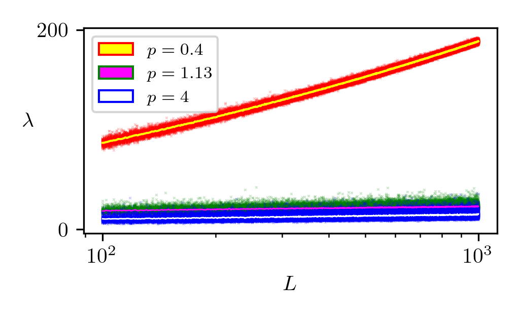
as previously defined in the main text (which again this choice tamed the semi-positiveness of $\rho$ ). This maps the spectrum of $\Gamma$ to the $[0,1]$ interval regardless of $p$ or $L$ . Thus, it is worth studying the behavior of $\lambda_{\text{max}}$ used for this definition of $\Gamma$ for different values of $p$ and $L$ , Figure 9. One finds that in the localized phase $\lambda_{\text{max}}$ remains roughly fixed at a constant value for all such $p$ and $L$ whereas in the thermal phase $\lambda_{\text{max}}$ grows as a power-law with $L$ .

5.2. Power-law decay of $\Gamma$ matrix elements

$\Gamma$ ’s matrix elements decay away from the diagonal as the distance to it, $d$ , is increased. This decay is intimately related to $p$ via

X_{jk}=\frac{x_{jk}}{(|j-k|+1)^{p}}.

(23)

As depicted in Figure 10, for large enough $d$ , the decay of the matrix elements of $\Gamma$ away from the diagonal is roughly given by

||\Gamma_{L/2,L/2+d}||\sim\frac{1}{d^{p}}\quad\text{for}\quad 1\ll d.

(24)

As $\Gamma$ is hermitian, this observation connects the localization transition of $\Gamma$ ’s eigenvectors to the already mentioned power-banded localized Hamiltonian models in the literature.

Figure 10: Log-log plot of the decay of the matrix elements of

\Gamma

as a distance

d

away from the diagonal. For large enough

d

, the decay is given by a power law with an exponent approximately equal to

p

. In the legend,

g

\log

, is the linear gradient of the black lines fitted to the log-log data. Note how

p\sim g

\log

, suggesting a power law decay with power

p

for large enough

d

5.3. Power-law decay of $\Gamma$ eigenvectors

Prior studies of PRBMs have observed power-law decay of eigenstates away from a central site, particularly closer to the transition within the localized phase. This is in contrast to eigenstates in short-range models exhibiting exponential decay. In Fig. 11 we present data suggesting our PRBM model exhibits the same phenomena, with small deviations from power-law behavior at lower values of $p$ .

Figure 11: (a-b) Five sample eigenstates with a maximum magnitude value within the middle 25th of the system at (a)

p=0.5

and (b)

p=1.1

. (c) Log-log plot of the averaged positional probability as a function of distance from the most probably site, for

p=[0.5,0.7,0.9,1.0,1.2,1.4,1.7,2.0]

. Averaged over eigenstates with most probable sites located in the middle 5th of the system, and averaged over

1000

disorder realizations. Linear fits of the probabilities for distances of

100

1000

are shown by the dashed lines. Inset: (solid) gradients of the linear fits are shown vs

p

, (dashed) the curve

y=p

6. Mutual information with boundaries

When we set to explore the mutual information behavior between two subsystems, one needs to choose whether or not to include the boundaries that separate these two subsystems. In the main text, we decided to exclude the boundaries between $A$ and $B$ so when $L\rightarrow\infty$ even if $A/L$ and $B/L$ are set constant the boundary $\partial_{AB}$ contribution to $\overline{\mathcal{I}}_{\infty}$ dies off as $\partial_{AB}$ grows. This is because it filters the very short-range entanglement contribution of $\partial_{AB}$ for sufficiently large $L$ . This can be seen in the area-law phase in Fig. 1 of the main text. Here we redo our analysis of the mutual information without removing $\partial_{AB}$ in Fig. 12. As expected, $p_{c}$ shifts into the area law phase as now the short-range entanglement is a more dominant contribution to $\overline{\mathcal{I}}_{\infty}$ . This also illustrates the strength of this contribution towards $\overline{\mathcal{I}}_{\infty}$ , which can be seen in this shift and the overall substantially larger magnitude of $\overline{\mathcal{I}}_{\infty}$ . Note that in contrast to the unusual $L_{A}$ dependence we observe in the case without boundary contributions, here we see a clear change from a sub-extensive power-law dependence at low $p$ to an area law dependence at high $p$ .

Figure 12: Steady state mutual information between

A

and

B

including their boundary term

\partial_{AB}

7. Numerical details

7.1. Disorder realizations

In Fig. 1 of the main text (b), disorder realizations are linearly decreased from $500$ at $L=100$ to $100$ at $L=1000$ . In (c), $20$ disorder realizations were used. Fig. 2 of the main text uses identical disorder realizations to Fig. 1. In Fig. 3 of the main text, from $L=400$ to $L=2000$ , disorder realizations were $[500,200,200,200,100]$ . The inset of Fig. 3 of the main text was done using identical numbers of disorder realizations.

Fig. 5 of the main text was computed by randomly generating $\Gamma$ at each $p$ , $10^{3}$ times, and from this obtaining the temperature distribution shown. The inset was computed at $L=[50,100,\cdots,1000]$ and averaged with disorder realizations $[2000,1900,\cdots,100]$ respectively for each value of $p$ .

Fig. 9 was computed by randomly sampling $X^{\dagger}X$ in the $L=[10^{2},10^{3}]$ interval $10^{5}$ times for each value of $p$ shown.

Fig. 10 was computed at $L=10^{3}$ and averaged over $10^{3}$ realizations.

7.2. Finite-size scaling

To perform a finite-size scaling analysis on the MI data, we optimize a standard loss function which measures the spread of the data, see e.g. Ref. Zabalo et al. 2020. Given our data possesses non-zero error bars from averaging over disorder realizations, we perform this analysis by sampling gaussian perturbations of our dataset, sampling noise for each data point with a standard deviation equal to the error in the mean for that data point. For each sample of a noise-perturbed dataset, we then optimize the loss to find a corresponding critical point and exponent. The expected value and variance of these resulting parameters are then calculated, using $1000$ noisy realizations of our dataset.