A generative model to synthetize spatio-temporal dynamics of biomolecules in cells

In order to mimic the dynamics of biomolecules, we consider a multitype birth-death-move process with mutations, denoted by $(\mathbf{X}_{t})_{t\geq 0}$.This process is a generalisation of birth-death-move processes, as introduced in [18]. In the following, to avoid misunderstanding we rather use the term “transformation” instead of “mutation”, as explained in Section 1. This section describes the spatio-temporal dynamics of $(\mathbf{X}_{t})_{t\geq 0}$ and introduces some notation.

At each time $t$, $\mathbf{X}_{t}$ is a collection of particles located in a bounded set $\Lambda$ of $\mathbb{R}^{d}$. Each particle is assigned a mark that represents a certain feature. We denote by $\mathbb{M}$ the collection of possible marks. Through time, the particles move (possibly depending on their associated mark and in interaction with each other) and three sudden changes may occur, that we call “jumps”:

1. 1.

   a “birth”: a new particle, assigned with a mark, may appear;

2. 2.

   a “death”: an existing particle may disappear;

3. 3.

   a “transformation”: the mark of an existing particle may change.

We denote by $n(\mathbf{X}_{t})$ the number of particles at time $t$. Each particle $x_{i}\in\mathbf{X}_{t}$, for $i=1,\dots,n(\mathbf{X}_{t})$, is decomposed as $x_{i}=(z_{i},m_{i})$ where $z_{i}\in\Lambda$ stands for its position while $m_{i}\in\mathbb{M}$ denotes its mark. Accordingly we have $\mathbf{X}_{t}\in(\Lambda\times\mathbb{M})^{n(\mathbf{X}_{t})}$. (Strictly speaking the ordering of particles in $\mathbf{X}_{t}$ does not matter, because any permutation of particles leads to the same collection of particles. We choose in this paper to bypass this nuance and use the same notation as if $\mathbf{X}_{t}$ was a vector a particles, even it is actually a set of particles.) Since the number of particles changes over time, the stochastic process $(\mathbf{X}_{t})_{t\geq 0}$ takes its values in the space

To stress the fact that $\mathbf{X}_{t}$ is not a simple value but encodes the positions and marks of a system of particles, we will say that this system at time $t$ is in configuration $\mathbf{X}_{t}$.

To fully specify the dynamics of $(\mathbf{X}_{t})_{t\geq 0}$, we need the following ingredients:

1. 1.

   A system of equations $(Move)$ that rules the way each particle of $\mathbf{X}_{t}$ moves continuously between two jumps. We will typically consider a system of stochastic differential equations acting on the position of each particle, possibly depending on their associated mark and in interaction with the other particles;

2. 2.

   Three continuous bounded functions $\beta$, $\delta$ and $\tau$ from $E$ to $[0,\infty)$, called birth, death and transformation intensity functions respectively, that govern the waiting times before a new birth, a new death and a new transformation. At each time $t$, we may interpret $\beta(\mathbf{X}_{t})dt$ as the probability that a birth occurs in the interval $[t,t+dt]$, given that the system of particles is in the configuration $\mathbf{X}_{t}$, and similarly for $\delta$ and $\tau$.

3. 3.

   Three transition probability functions that indicate how each jump occurs:

   • •

     $p^{\beta}((z,m)|\mathbf{x})$: probability density function that the birth occurs at the position $z$ with the mark $m$, given that there is a birth and that the system of particles is in configuration $\mathbf{x}$ at the birth time;

   • •

     $p^{\delta}(x_{i}|\mathbf{x})$, for $x_{i}\in\mathbf{x}$: probability that the death concerns the particle $x_{i}$ in $\mathbf{x}$, given that there is a death and that the system of particles is in configuration $\mathbf{x}$ at the death time;

   • •

     $p^{\tau}((z_{i},m_{i}),m|\mathbf{x})$, for $(z_{i},m_{i})\in\mathbf{x}$: probability that the particle $x_{i}=(z_{i},m_{i})$ in $\mathbf{x}$ changes its mark and that this transformation leads to the new mark $m\neq m_{i}$, given that there is a transformation and that the system of particles is in configuration $\mathbf{x}$ at the transformation time.

We provide in Section 2.3 some examples for the choice of these characteristics. Finally, we will denote by $T_{1},T_{2},\dots$ the jump times of the process and we agree that $T_{0}=0$.

Assume we are given the characteristics of the process $(\mathbf{X}_{t})_{t\geq 0}$ as introduced in the previous section, that are the system of equations $(Move)$, the intensity functions $\beta$, $\delta$, $\tau$, and the transition probability functions $p^{\beta}$, $p^{\delta}$, $p^{\tau}$. Then, starting from an initial configuration $\mathbf{X}_{0}$ at time $T_{0}=0$, we construct iteratively the process in the time interval $[0,T]$ as follows. Here we set $\alpha=\beta+\delta+\tau$ to be the total intensity of jumps.

1. 1.

   Generate $n(\mathbf{X}_{0})$ continuous trajectories as solutions of $(Move)$ in the interval $[0,T-T_{0}]$, given the initial conditions $\mathbf{X}_{0}$. Denote $(\mathbf{Y}_{t})_{t\in[0,T-T_{0}]}$ these trajectories.

2. 2.

   By flipping a coin, test whether the jump time $T_{1}$ occurs after $T$ (this is with probability $p$) or before $T$ (this is with probability $1-p$), where

   $$p=\exp\left(-\displaystyle\int_{0}^{T-T_{0}}\alpha(\mathbf{Y}_{u})du\right).$$

   • •

     If $T_{1}>T$, then $\mathbf{X}_{t}=\mathbf{Y}_{t-T_{0}}$ for all $t\in[T_{0},T]$, which completes the simulation.

   • •

     Otherwise, we continue by generating $T_{1}$ in $[T_{0},T]$ and the associated jump as in the following.

3. 3.

   Generate $T_{1}-T_{0}$, given that $T_{1}<T$, according to the probability distribution

   $$\mathbb{P}(T_{1}-T_{0}<t|T_{1}<T)=\frac{1}{1-p}\left(1-\exp\left(-\displaystyle\int_{0}^{t}\alpha(\mathbf{Y}_{u})du\right)\right),\quad 0<t<T-T_{0}.$$

   The process until the time $T_{1}$ is then given by the generated trajectories, i.e.

   $$(\mathbf{X}_{t})_{T_{0}\leq t<T_{1}}=(\mathbf{Y}_{t-T_{0}})_{T_{0}\leq t<T_{1}}.$$

4. 4.

   Draw which kind of jump occurs at $T_{1}$ (we denote by $\mathbf{X}_{T_{1}^{-}}$ the configuration of the process just before the jump, which is $\mathbf{Y}_{T_{1}-T_{0}}$ by continuity of $(\mathbf{Y}_{t})$):

   • •

     this is a birth with probability $\beta(\mathbf{X}_{T_{1}^{-}})/\alpha(\mathbf{X}_{T_{1}^{-}})$;

   • •

     this is a death with probability $\delta(\mathbf{X}_{T_{1}^{-}})/\alpha(\mathbf{X}_{T_{1}^{-}})$;

   • •

     this is a transformation with probability $\tau(\mathbf{X}_{T_{1}^{-}})/\alpha(\mathbf{X}_{T_{1}^{-}})$.

5. 5.

   Generate the jump at $t=T_{1}$ to get $\mathbf{X}_{T_{1}}$ as follows:

   • •

     if this is a birth, generate the new particle $x=(z,m)$ according to the probability density function $p^{\beta}((z,m)|\mathbf{X}_{T_{1}^{-}})$. Then set $\mathbf{X}_{T_{1}}=\mathbf{X}_{T_{1}^{-}}\cup(z,m)$;

   • •

     if this is a death, draw which particle $x_{i}\in\mathbf{X}_{T_{1}^{-}}$ to delete according to the probability $p^{\delta}(x_{i}|\mathbf{X}_{T_{1}^{-}})$, for $i=1,\dots,n(\mathbf{X}_{T_{1}^{-}})$. Then set $\mathbf{X}_{T_{1}}=\mathbf{X}_{T_{1}^{-}}\setminus x_{i}$;

   • •

     if this is a transformation, draw which particle $x_{i}=(z_{i},m_{i})\in\mathbf{X}_{T_{1}^{-}}$ is transformed and generate its transformation according to $p^{\tau}((z_{i},m_{i}),m|\mathbf{X}_{T_{1}^{-}})$, for $i=1,\dots,n(\mathbf{X}_{T_{1}^{-}})$. Then set $\mathbf{X}_{T_{1}}=(\mathbf{X}_{T_{1}^{-}}\setminus(z_{i},m_{i}))\cup(z_{i},m)$.

6. 6.

   Back to step 1 with $T_{0}\leftarrow T_{1}$ and $\mathbf{X}_{0}\leftarrow\mathbf{X}_{T_{1}}$ in order to generate the new trajectories starting from $\mathbf{X}_{T_{1}}$ and the next jump time $T_{2}$, and so on.

In the first step of the above construction, the trajectories are generated up to the final time $T$. It is however very likely that the next jump occurs much before $T$ so that it would be sufficient and computationally more efficient to generate these trajectories on a shorter time interval. We provide in Appendix a formal algorithm of simulation of $\mathbf{X}_{t}$ for $t\in[0,T]$, following the above construction and including the latter idea. This algorithm has been implemented in Python and is available in our GitHub repository.

From a theoretical side, note that the specific exponential form of the probability distribution of the inter-jump waiting time in step 3 is necessary to imply the interpretation of $\beta$, $\delta$ and $\tau$ explained in the previous section. This exponential form also implies that $(\mathbf{X}_{t})_{t\geq 0}$ is a Markov process, meaning that its future dynamics only depends on its present configuration. We refer to [18] for more details about these theoretical aspects.

The dataset we consider comes from the observation by a 3D multi-angle TIRF (total internal reflection fluorescence) microscopy technique of the intracellular trafficking of m-Cherry Langerin and GFP Rab11 proteins in a RPE1 living cell [3], specifically projected along the z-axis onto the 2D plane close to the plasma membrane. This provides a 2D image sequence of 1199 frames, each lasting 140 ms and showing the simultaneous locations of the two types of proteins. The two images at the top of Figure 2 depict the first frame of the raw sequence for the Langerin fluorescent channel and the Rab11 fluorescent channel, respectively, recorded simultaneously using a dual-view optical device. Note that the cell adheres on a fibronectin micropattern, which constrains intracellular constituents such as cytoskeleton elements and gives a reproducible shape, explaining the “umbrella” shape of the cell. These raw sequences are post-processed following [22; 21], then each bright spot is represented by a single point, and we apply the U-track algorithm [11] to estimate particle trajectories. The bottom images of Figure 2 show the resulting trajectories for the Langerin channel and the Rab11 channel, respectively. These trajectories have been further analysed by the method developed in [6] to classify them into three diffusion regimes: Brownian, superdiffusive and subdiffusive, which corresponds to the blue, red and green colors, respectively, in Figure 2.

To be more specific in the analysis of all trajectories, we fit three parametric models to each of them, following [6], depending on their regime:

1. 1.

   For a Brownian regime (in blue): a Brownian motion,

2. 2.

   for a superdiffusive regime (in red): a Brownian motion with constant drift,

3. 3.

   for a subdiffusive regime (in green): an Ornstein-Uhlenbeck process.

Each trajectory has its individual parameters (see Examples 2.3.1 and 2.3.1), estimated by maximum likelihood. Furthermore, some trajectories may change from one regime to another, which corresponds to a “transformation” in the BDM model that will be specified in the next section.

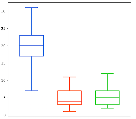
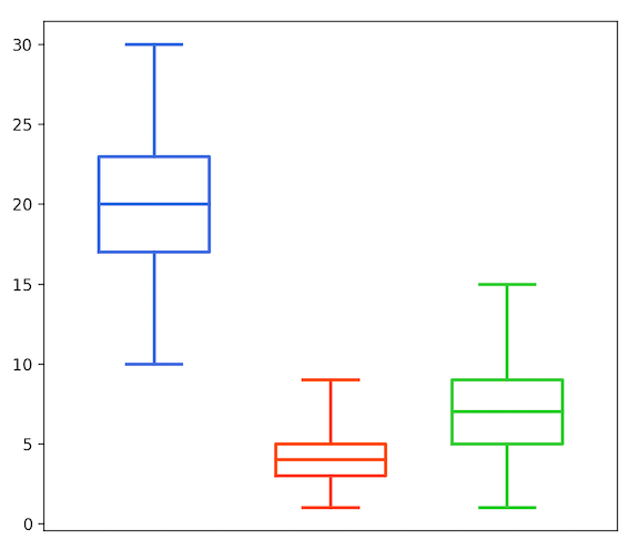
Figure 3 summarises different features of the obtained trajectories for the Langerin sequence (the same characteristics have been analysed for the Rab11 sequence, but are not detailed here). The histograms at the bottom display the duration of all trajectories (in frames), according to their regime. We can observe that the (blue) Brownian and (red) superdiffusive trajectories have quite a short lifetime in average, in comparison with the subdiffusive trajectories (in green). The top-right boxplots represent the distribution of the number of particles per frame, according to their regime: there is a majority of Brownian motions, followed by subdiffusive motions and a minority of superdiffusive motions. Finally, the top-left circular histogram aims at depicting the orientation of the drift vectors for the superdiffusive (red) trajectories. Specifically, for this plot, we have recorded the deviation of the drift angle (in degrees) with respect to the direction towards the center of the cell. For instance this deviation is $0^{\circ}$ if the drift goes towards the center, and $180^{\circ}$ if it goes in the opposite direction. It appears from this plot that most deviation angles are around $0^{\circ}$ or $180^{\circ}$, meaning that the red trajectories mainly move in a radial direction going to (or starting from) the center of the cell.

The above descriptors will be helpful to calibrate the parameters of the BDM model in the next section and they will also serve as benchmarks to evaluate the quality of our simulations. However it is important to keep in mind that they come with some approximations and errors induced by imperfect tracking algorithms. In particular, no trajectory can last less than 10 frames in the data, which is a minimal length of detection for our tracking method. It is also clear in the bottom plots of Figure 2, that some directed (superdiffusive) trajectories appear wrongly in blue, which can be explained by the multiple testing procedure of [6] that aims at minimizing the number of false positives (that are bad green or bad red trajectories) to the detriment of possibly too many false negatives (that are wrong blue trajectories).

Concerning the births and deaths of trajectories, we summarize in Table 1 their total numbers observed in the real-dataset, according to the type of proteins and motion regime. The number of regime transformations is in turn given in Table 2 for the Langerin proteins. For the Rab11 proteins, only one switching from a Brownian motion to a subdiffusive motion was observed during the sequence.

To address in detail these jumps dynamics, we leverage the study carried out for the same dataset in [18], where it has been concluded that for each type of proteins and motion regimes, the birth intensity is constant, like in Example 2.3.2, while the death intensity is proportional to the number of existing particles, like in Example 2.3.2. Given the small number of observed motion regime transformations, its intensity can also be considered as constant. Concerning the transition probability functions, the deaths occur uniformly over all existing particles, like in Example 2.3.3. As to the birth transition, there is no reason to choose another density than the uniform distribution over the cell for the Rab11 proteins (Example 2.3.3). But due to colocalization (as observed for this dataset in [19]), the birth density for the Langerin positive structures can be approximated by a mixture between a uniform distribution, for $93\%$ of the Langerin births, and a colocalized density around the existing Rab11 vesicles, like in Example 2.3.3, for $7\%$ of the Langerin births. These proportions, along with the other parameters, have been estimated by maximum likelihood.

References

- [1] Badoual, A., Arizono, M., Denizot, A., Ducros, M., Berry, H., Nägerl, U. V., and Kervrann, C. Simulation of astrocytic calcium dynamics in lattice light sheet microscopy images. In 2021 IEEE 18th International Symposium on Biomedical Imaging (ISBI) (2021), IEEE, pp. 135–139.
- [2] Bolte, S., and Cordelieres, F. A guided tour into subcellular colocalization analysis in light microscopy. J Microscopy 224 (2006), 213–232.
- [3] Boulanger, J., Gueudry, C., Munch, D., Cinquin, B., Paul-Gilloteaux, P., Bardin, S., Guérin, C., Senger, F., Blanchoin, L., and Salamero, J. Fast high-resolution 3D total internal reflection fluorescence microscopy by incidence angle scanning and azimuthal averaging. Proc Natl Acad Sci USA 111, 48 (2014), 17164–17169.
- [4] Boulanger, J., Kervrann, C., and Bouthemy, P. A simulation and estimation framework for intracellular dynamics and trafficking in video-microscopy and fluorescence imagery. Medical image analysis 13, 1 (2009), 132–142.
- [5] Bressloff, P. C., and Newby, J. M. Stochastic models of intracellular transport. Reviews of Modern Physics 85, 1 (2013), 135.
- [6] Briane, V., Kervrann, C., and Vimond, M. Statistical analysis of particle trajectories in living cells. Phys Rev E. 97, (6-1):062121 (2018).
- [7] Briane, V., Vimond, M., and Kervrann, C. An overview of diffusion models for intracellular dynamics analysis. Briefings in Bioinformatics (2019). bbz052.
- [8] Chenouard, N., Smal, I., De Chaumont, F., Maška, M., Sbalzarini, I. F., Gong, Y., Cardinale, J., Carthel, C., Coraluppi, S., Winter, M., et al. Objective comparison of particle tracking methods. Nature methods 11, 3 (2014), 281–289.
- [9] Costes, S., Daelemans, D., Cho, E., Dobbin, Z., Pavlakis, G., and Lockett, S. Automatic and quantitative measurement of protein-protein colocalization in live cells. Biophysical J 86, 6 (2004), 3993–4003.
- [10] Hozé, N., and Holcman, D. Statistical methods for large ensembles of super-resolution stochastic single particle trajectories in cell biology. Annual Review of Statistics and Its Application 4 (2017), 189–223.
- [11] Jaqaman, K., Loerke, D., Mettlen, M., Kuwata, H., Grinstein, S., Schmid, S. L., and Danuser, G. Robust single-particle tracking in live-cell time-lapse sequences. Nature methods 5, 8 (2008), 695.
- [12] Kervrann, C. Biomolecule trafficking and network tomography-based simulations. In Biomedical Image Synthesis and Simulation. Elsevier, 2022, pp. 543–569.
- [13] Kervrann, C., Sorzano, C. Ó. S., Acton, S. T., Olivo-Marin, J.-C., and Unser, M. A guided tour of selected image processing and analysis methods for fluorescence and electron microscopy. IEEE Journal of Selected Topics in Signal Processing 10, 1 (2015), 6–30.
- [14] Lagache, T., Dauty, E., and Holcman, D. Quantitative analysis of virus and plasmid trafficking in cells. Physical Review E 79, 1 (2009), 011921.
- [15] Lagache, T., Sauvonnet, N., Danglot, L., and Olivo-Marin, J.-C. Statistical analysis of molecule colocalization in bioimaging. Cytometry Part A 87, 6 (2015), 568–579.
- [16] Lagardère, M., Chamma, I., Bouilhol, E., Nikolski, M., and Thoumine, O. Fluosim: simulator of single molecule dynamics for fluorescence live-cell and super-resolution imaging of membrane proteins. Scientific Reports 10, 1 (2020), 1–14.
- [17] Lavancier, F., Le Guével, R., and Manent, E. Feller and ergodic properties of jump-move processes with applications to interacting particle systems. arXiv preprint arXiv:2204.02851 (2022).
- [18] Lavancier, F., and Le Guével, R. Spatial birth–death–move processes: basic properties and estimation of their intensity functions. Journal of the Royal Statistical Society: Series B (Statistical Methodology) 83, 4 (2021), 798–825.
- [19] Lavancier, F., Pécot, T., Zengzhen, L., and Kervrann, C. Testing independence between two random sets for the analysis of colocalization in bioimaging. Biometrics 76, 1 (2020), 36–46.
- [20] Øksendal, B. Stochastic differential equations: an introduction with applications. Springer Science & Business Media, 2013.
- [21] Pécot, T., Bouthemy, P., Boulanger, J., Chessel, A., Bardin, S., Salamero, J., and Kervrann, C. Background fluorescence estimation and vesicle segmentation in live cell imaging with conditional random fields. IEEE Transactions on Image Processing 24, 2 (2014), 667–680.
- [22] Pécot, T., Kervrann, C., Bardin, S., Goud, B., and Salamero, J. Patch-based markov models for event detection in fluorescence bioimaging. In International Conference on Medical Image Computing and Computer-Assisted Intervention (2008), Springer, pp. 95–103.
- [23] Pécot, T., Zengzhen, L., Boulanger, J., Salamero, J., and Kervrann, C. A quantitative approach for analyzing the spatio-temporal distribution of 3d intracellular events in fluorescence microscopy. eLife 7 (2018), e32311.
- [24] Roudot, P., Ding, L., Jaqaman, K., Kervrann, C., and Danuser, G. Piecewise-stationary motion modeling and iterative smoothing to track heterogeneous particle motions in dense environments. IEEE Transactions on Image Processing 26, 11 (2017), 5395–5410.