Transition behavior of the waiting time distribution in a jumping model with the internal state

Zhe Xue Affiliation: School of Mathematical Sciences and Institute of Natural Sciences, MOE-LSC, CMA-Shanghai, Shanghai Jiao Tong University, China Yuan Zhang Thanks: Corresponding author: zhang_probab@ruc.edu.cn Affiliation: Center for Applied Statistics and School of Statistics, Renmin University of China, China Affiliation: Pazhou Laboratory, Guangzhou 510330, China Zhennan Zhou Affiliation: Beijing International Center for Mathematical Research, Peking University, China Min Tang Thanks: Corresponding author: tangmin@sjtu.edu.cn Affiliation: School of Mathematical Sciences and Institute of Natural Sciences, MOE-LSC, CMA-Shanghai, Shanghai Jiao Tong University, China

Abstract

It has been noticed that when the waiting time distribution exhibits a transition from an intermediate time power law decay to a long-time exponential decay in the continuous time random walk model, a transition from anomalous diffusion to normal diffusion can be observed at the population level. However, the mechanism behind the transition of waiting time distribution is rarely studied. In this paper, we provide one possible mechanism to explain the origin of such transition. A jump model terminated by a state-dependent Poisson clock is studied by a formal asymptotic analysis for the time evolutionary equation of its probability density function. The waiting time behavior under a more relaxed setting can be rigorously characterized by probability tools. Both approaches show the transition phenomenon of the waiting time $T$ , which is further verified numerically by particle simulations. Our results indicate that a small drift and strong noise in the state equation and a stiff response in the Poisson rate are crucial to the transitional phenomena.

Keywords: power-law decay; exponential decay; waiting time; transitional phenomena

1 Introduction

Diffusion processes are continuous-time, continuous-state processes whose sample paths are everywhere continuous but nowhere differentiable [10, 11, 20]. One can classify the diffusion process into normal diffusion and anomalous diffusion depending on whether the Fick’s laws are obeyed [7]. Interestingly, a transition from anomalous diffusion to normal diffusion can be observed in many systems, for example, viscoelastic systems such as lipid bilayer membranes, systems of actively moving biological cells [12, 17] or particles adsorbed in the internal walls of porous deposits [21], etc.

The most popular model to study the diffusion processes is the continuous time random walk (CTRW) model which was originally introduced by Montroll and Weiss [18, 15]. The CTRW model considers a particle that starts at the origin and consecutively jumps to different positions. The particle waits for a trapping time $\Delta t$ at each position and then jumps to another position whose distance from the previous position is $\Delta x$ . Here, $\Delta t$ and $\Delta x$ are two random variables (r.v.’s) whose probability density distributions (PDF) are respectively $\Psi(\Delta t)$ and $\Phi(\Delta x)$ , and there is no bias in the jumping direction [9, 2, 16]. When the first moment of the waiting time and the variance of the jumping length are finite, the CTRW model gives normal diffusion. When the variance of the jumping length is finite but the waiting time distribution has a tail that decays according to the power law, i.e.

\Psi(\Delta t)\sim\frac{1}{\Delta t^{1+\alpha}},\quad\Delta t\to\infty,

(1.1)

with $0<\alpha<1$ , the CTRW model leads to sub-diffusion [6, 22]. When all moments of $\Psi(\Delta t)$ are finite and $\Phi(\Delta x)\simeq 1/|\Delta x|^{1+\alpha}$ with $0<\alpha<2$ , this will lead to a super-diffusion [13, 6].

The transition from anomalous diffusion to normal diffusion can be modeled by CTRW model as well. For example, the authors in [6] study a CTRW model with the jumping length being the absolute value of a normal distribution and the waiting time distribution $\Psi(\Delta t)$ being

\Psi(\Delta t)\propto\exp\left(-\frac{\Delta t}{t_{2}}\right)\left(1+\frac{\Delta t}{t_{1}}\right)^{-(1+\beta)},

(1.2)

where $t_{1}\ll t_{2}$ are two time scales and $0<\beta<2$ is a constant. When $t_{1}\ll\Delta t\ll t_{2}$ , $\Psi(\Delta t)$ has a power-law decay with respect to $\Delta t$ , i.e. $\Psi(\Delta t)\propto(\Delta t/t_{1})^{-(1+\beta)}$ , while when $t\gg t_{2}$ , $\Psi(\Delta t)$ decreases exponentially fast. As has been pointed out in [6], one can observe that $\Psi(\Delta t)$ as in (1.2) induces the transition from anomalous diffusion to normal diffusion at the population level, which indicates that the transition from intermediate-time power-law decay to long-time exponential decay in waiting time distribution is highly related to the transitions from anomalous diffusion to normal diffusion.

One natural question is why the waiting time distribution may transit from the intermediate-time power-law decay to the long-time exponential decay. Motivated by the model and simulations in [24] which studies the rotational directions of bacteria flagella, we propose a jump process controlled by the internal state and show that this transition can be induced by a small drift and a strong noise in the internal state. The construction of this model is also partially inspired by recent studies of the firing mechanism of neurons [26, 14]. We consider particles staying inside a potential well whose internal states $X_{t}$ evolve according to an Ornstein–Uhlenbeck (OU) process, where the strength of the drift is assumed to be of a lower order scale. The particles can jump outside of the potential well by a state-dependent Poisson process whose rate $\Lambda(x)$ equals to (or rapidly converges to) zero on one half of the $x$ -axis and is uniformly bounded away from zero on the other half. We find out that the waiting time distribution of the particles staying inside the well exhibits a transition from an intermediate-time power-law decay to a long-time exponential decay.

We explore the transitional phenomenon from two approaches: one is a formal asymptotic analysis for the partial differential equation (PDE) describing the time evolution of the probability density function of $X_{t}$ , and the other is a rigorous quantitative estimate by the probability tools. In the PDE approach, we can obtain the leading order behavior of the density distribution function in two different time regimes. The decay profile of the waiting time distribution in these two distinct regimes can be given analytically. However, this approach replies on explicit calculations that are only applicable to some special cases. The probability approach, on the other hand, applies to more general rate functions and similar results can be proved by estimating upper bounds and lower bounding for cumulative distribution of the stopping time.

The paper is organized as follows. In Section 2, we first review the two state model for the E.Coli flagella rotational direction in [24] and propose a simplified one state jump model controlled by the internal state, then the main results are summarized. The PDE that describes the time evolution of the probability density function is studied in Section 3. We use Laplace transform and formal asymptotics to get the leading order of the waiting time distribution. In Section 4, the main theorem is proved by using the probability tool. To verify the theoretical results, Section 5 is devoted to the numerical simulations of the jump process. Finally, we summarize the paper and discuss future directions in Section 6.

2 The model and the main results

2.1 The model

Each E.Coli cell has 6-8 flagella that can rotate either clockwise (CW) or counter-clockwise (CCW). The rotational directions of flagella control the movement of the E.Coli cells. When most of the motors rotate CCW, the flagella form a bundle and push the cell to run in a straight line. When one or more of the motors rotate CW, the cell tumbles without moving [25]. In [24], the authors model the switches between CW and CCW by a two state model, in which the switching rates are determined by the CheY-P concentration. CheY-P is an intracellular protein whose concentration evolves according to an Ornstein–Uhlenbeck (OU) process such that

dY(t)=-\frac{Y(t)-Y_{0}}{\tau}dt+dB(t),

(2.1)

where $Y(t)$ is the CheY-P concentration; $Y_{0}$ is a constant; $\tau$ is the CheY-P correlation time and $B(t)$ is the white noise. The switching rates from CCW to CW and CW to CCW are respectively

\Lambda_{0}(Y)\propto\exp\left(-\alpha_{0}\frac{Y(t)-Y_{0}}{Y_{0}}\right),\quad\Lambda_{1}(Y)\propto\exp\left(-\alpha_{1}\frac{Y(t)-Y_{0}}{Y_{0}}\right),

(2.2)

in which $\alpha_{0}$ and $\alpha_{1}$ are two constants. The authors find that when one uses large $\tau$ in (2.1) and large $\alpha_{0}$ in (2.2), the distribution of the CCW duration time decays according to a power-law.

In this paper, we focus on the CCW state and study a simplified one state model which is a jump process inside one potential well. The jump process is controlled by the internal state $X_{t}$ that satisfies an OU process:

dX_{t}=-\epsilon X_{t}dt+\sqrt{2}dB_{t}.

(2.3)

Here $\epsilon$ is a small drift corresponding to large $\tau$ in (2.1), $B_{t}$ is the white noise and $Y_{0}$ is chosen to be $0$ in (2.1). $X_{t}$ is terminated by a state-dependent Poisson clock with a jumping rate $\Lambda(X_{t})$ . We choose the jump rate $\Lambda(X_{t})$ to increase rapidly from zero to a positive number in line with (2.2). This will allow us to imitate the sharp transition when using large $\alpha_{0}$ in $\Lambda_{0}(Y)$ . More specifically, let $\Lambda(X_{t})$ be a nonnegative bounded measurable function supported on $[0,+\infty)$ such that

\Lambda(X_{t})\geq C_{+}>0,\quad\text{for $X_{t}\geq 0$},\qquad\Lambda(X_{t})=0,\quad\text{for $X_{t}<0$}.

(2.4)

Consider a stopping time $T$ :

T=\inf\left\{t:\int_{0}^{t}\Lambda(X_{s})ds>\Gamma\right\},

(2.5)

where $\Gamma\sim\exp(1)$ is an exponentially distributed random variable with rate $\lambda_{\Gamma}=1$ . $\Gamma$ is independent of $X_{t}$ . Let $\mathcal{F}_{t}$ be the $\sigma$ -algebra generated by $X_{s}$ : $s\leq t$ , one has

\mathbb{P}(T>t|\mathcal{F}_{t})=\mathbb{P}\left(\left.\int_{0}^{t}\Lambda(X_{s})ds\leq\Gamma\right|\mathcal{F}_{t}\right)=e^{-\int_{0}^{t}\Lambda(X_{s})ds}.

And given $\mathcal{F}_{t}$ , the conditional jumping rate at time $t$ is given by

\frac{\frac{d\mathbb{P}(T\leq t|\mathcal{F}_{t})}{dt}}{\mathbb{P}(T>t|\mathcal{F}_{t})}=\frac{\Lambda(X_{t})e^{-\int_{0}^{t}\Lambda(X_{s})ds}}{e^{-\int_{0}^{t}\Lambda(X_{s})ds}}=\Lambda(X_{t}).

At time $T$ , the OU process is terminated and $X_{t}$ is set to a frozen state say $-\infty$ afterward. In other words, the above dynamics can be equivalently seen as the OU process is killed at a state-dependent Poisson rate $\Lambda(X_{t})$ . The termination of the OU process can be considered as the switching from CCW to CW in the two-state model[24]. The killing time $T$ represents the CCW or CW duration time.

The PDE model.

Let $f(x,t)$ be the PDF of $X_{t}$ . By Dynkin’s formula [8], $f(x,t)$ satisfies the following Fokker-Planck equation

\begin{cases}\frac{\partial f}{\partial t}-\epsilon\frac{\partial}{\partial x}(xf)-\frac{\partial^{2}f}{\partial x^{2}}=-\Lambda(x)f,\\ f(x,0)=\delta(0),\end{cases}

(2.6)

where $\Lambda(x)$ is the same as in (2.4) after replacing $X_{t}$ by $x$ . The probability that the particle has not jumped up to time $t$ is

N(t)=\int_{-\infty}^{\infty}f(x,t)dx.

The PDF of the waiting time distribution is given by [5, 4, 3]

n(t)=-\frac{d}{dt}N(t)=-\int_{-\infty}^{\infty}\frac{\partial}{\partial t}f(x,t)dx.

From (2.6), one has

n(t)=\int_{-\infty}^{\infty}\Lambda(x)f(x,t)dx,

(2.7)

where $\Lambda(x)$ is defined as in (2.4).

2.2 Main results

We study the waiting time distribution from two different perspectives: an asymptotic analysis based on the Fokker-Planck equation (2.6) and a rigorous proof by the probability tools. The main results are listed below.

In the PDE approach, we focus on the case that $\Lambda(x)$ is the following piece-wise constant function:

\Lambda(x)=\begin{cases}1&\text{$x\geq 0$},\\ 0&\text{$x<0$},\end{cases}

(2.8)

and in this case the PDF of the waiting time distribution is further simplified to

n(t)=\int_{0}^{\infty}f(x,t)dx.

We have derived the leading order behavior of the waiting time PDF as follows.

Proposition 2.1.

Let $f(x,t)$ satisfy the Fokker-Planck equation (2.6) with the rate function given by (2.8). When $\epsilon\to 0^{+}$ , the waiting time distribution $n(t)$ as in (2.7) satisfies

(1)

In an intermediate time scale $t=O(1)$ and $t<O(\frac{1}{\epsilon})$ , the waiting time distribution $n(t)\sim t^{-\frac{3}{2}}$ .
(2)

In a long time scale $t=O(\frac{1}{\epsilon^{2}})$ , the waiting time distribution $n(t)\sim e^{-t}$ .

For more general rate functions $\Lambda(X_{t})$ as in (2.4), we have the following estimates for the waiting time in similar time regimes.

Theorem 2.1.

Let $X_{t}$ satisfy the process (2.3) and be terminated by the state dependent Poisson clock with intensity $\Lambda(X_{t})$ that satisfies (2.4). Then for the waiting time $T$ defined in (2.5), we have

(a)

For any $\alpha\in(0,\frac{1}{6})$ , there exits a positive constant $M=M(\alpha)<\infty$ depending only on $\alpha$ such that

$\mathbb{P}(T>t)\geq\frac{1}{2}t^{-\frac{1}{2}-\alpha},\quad\forall t\in[M,\epsilon^{-\frac{1}{2}}],$

for sufficiently small $\epsilon$ .
(b)

There exists a positive constant $c>0$ such that

$\mathbb{P}(T>t)\leq\exp(-ct),$

with $t\in(\frac{1}{\epsilon^{2}},+\infty)$ for sufficiently small $\epsilon$ .

It is worth noting that the proof of Theorem 2.1 relies on the following characteristics of rate function $\Lambda$ :

1)

$\Lambda$ equals to or converges to $0$ on a half of the $x$ -axis, which, combined with a sufficiently small drift term, provides an almost Brownian environment that generates the power law decay in the macroscopic scale;
2)

$\Lambda$ is uniformly bounded away from $0$ on the other half of the axis, which leads to a positive probability of triggering the stopping time for an excursion into this half. Thus the exponential decay in the long run follows by the gambler’s ruin.

Our analytical results indicate that when $\tau$ is infinity in (2.1), i.e. when the CheY-P concentration has infinite time correlation, the waiting time distribution has a power-law decay tail, while when $\tau\gg 1$ but not infinity, there exhibits a transition from an intermediate-time power-law to a long-time exponential decay, the transitional time is at least at the order of $\sqrt{\tau}$ . In fact, our numerical tests in Section 5 seem to suggest that the transition takes place around $O(\tau)$ time.

3 Asymptotic analysis of the PDE model

To understand the behavior of $n(t)$ at different time scales, we look at the Laplace transform of $n(t)$ . From the definition of the Laplace transform

\hat{n}(s)=\int_{0}^{\infty}n(t)e^{-ts}dt,

it is easy to find that $\hat{n}(\frac{s}{\alpha})=\alpha\int_{0}^{\infty}n(\alpha t)e^{-ts}dt$ , with $\alpha$ being a constant. This indicates that when $\alpha\sim O(1)$ , i.e. $\frac{s}{\alpha}\sim O(1)$ , we are considering the intermediate time scale $t\sim O(1)$ , while when $\alpha=\frac{1}{\epsilon^{2}}$ , i.e. $\frac{s}{\alpha}\sim O(\epsilon^{2})$ , we are considering the long time scale $t\sim O(\frac{1}{\epsilon^{2}})$ . Therefore in the subsequent part, we calculate the explicit expression of $\hat{n}(s)$ and find its asymptotic approximations when $s\sim O(1)$ and $s\sim O(\epsilon^{2})$ .

3.1 The explicit formula of $\hat{n}(s)$

Taking Laplace transform on both sides of (2.6) yields

\hat{f}^{{}^{\prime\prime}}+\epsilon x\hat{f}^{{}^{\prime}}+[\epsilon-s-\Lambda(x)]\hat{f}=-f(x,0)=\delta(0),

(3.1)

where $\hat{f}(x,s)$ is the Laplace transform of $f(x,t)$ and ^′ is the derivative with respect to $x$ .

Letting $\hat{f}_{+}(x)=\hat{f}(x)|_{x\in(0,+\infty)}$ and $\hat{f}_{-}(x)=\hat{f}(x)|_{x\in(-\infty,0)}$ , (3.1) can be rewritten into the following two equations:

	$\hat{f}_{+}^{{}^{\prime\prime}}+\epsilon x\hat{f}_{+}^{{}^{\prime}}+[\epsilon-(s+1)]\hat{f}_{+}=0,$		(3.2a)
	$\hat{f}_{-}^{{}^{\prime\prime}}+\epsilon x\hat{f}_{-}^{{}^{\prime}}+[\epsilon-s]\hat{f}_{-}=0.$		(3.2b)

$\hat{f}_{+}$ and $\hat{f}_{-}$ are connected at $x=0$ by

\lim_{x\to 0^{+}}\hat{f}_{+}(x)=\lim_{x\to 0^{-}}\hat{f}_{-}(x),\quad\lim_{x\to 0^{+}}\hat{f}_{+}^{{}^{\prime}}(x)-\lim_{x\to 0^{-}}\hat{f}_{-}^{{}^{\prime}}(x)=-1.

(3.3)

We solve $\hat{f}_{+}$ and $\hat{f}_{-}$ in the subsequent part.

Solve $\hat{f}_{+}(x,s)$ .

By introducing $y=\sqrt{\epsilon}x$ and $\hat{H}_{+}(y,s)=e^{\frac{\epsilon}{4}x^{2}}\hat{f}_{+}(x,s)$ , (3.2a) can be written into

\hat{H}_{+}^{{}^{\prime\prime}}-\left(\frac{y^{2}}{4}+\frac{s+1}{\epsilon}-\frac{1}{2}\right)\hat{H}_{+}=0.

(3.4)

(3.4) is of the form of parabolic cylinder function in (B.1). From Appendix B, (3.4) has two general solutions

\displaystyle\hat{H}_{+,1}(y)

\displaystyle={}U\left(\frac{s+1}{\epsilon}-\frac{1}{2},y\right)=\sqrt{\pi}2^{-\frac{s+1}{2\epsilon}}\left[\frac{h_{1}(y)}{\Gamma(\frac{s+1}{2\epsilon}+\frac{1}{2})}-\frac{\sqrt{2}h_{2}(y)}{\Gamma(\frac{s+1}{2\epsilon})}\right],

(3.5)

	$\displaystyle\hat{H}_{+,2}(y)$	$\displaystyle={}V\left(\frac{s+1}{\epsilon}-\frac{1}{2},y\right)=\frac{2^{-\frac{s+1}{2\epsilon}}}{\sqrt{\pi}\Gamma(1-\frac{s+1}{\epsilon})}\left[\sin(\frac{s+1}{2\epsilon}\pi)\Gamma(\frac{1}{2}-\frac{s+1}{2\epsilon})h_{1}(y)\right.$
		$\displaystyle+{}\left.\sqrt{2}\cos(\frac{s+1}{2\epsilon}\pi)\Gamma(1-\frac{s+1}{2\epsilon})h_{2}(y)\right].$		(3.6)

where

h_{1}(y)=e^{-\frac{\epsilon}{4}x^{2}}M\left(\frac{s+1}{2\epsilon},\frac{1}{2},\frac{y^{2}}{2}\right),\quad h_{2}(y)=ye^{-\frac{\epsilon}{4}x^{2}}M\left(\frac{1}{2}+\frac{s+1}{2\epsilon},\frac{3}{2},\frac{y^{2}}{2}\right).

Here $M(a,b,x)$ is the Kummer’s function, whose useful properties are listed in Appendix A; $U(a,y)$ , $V(a,y)$ are called the parabolic cylinder functions whose properties are listed in Appendix B.

By the properties of the parabolic cylinder functions as in (B.4) and (B.5), when $y\to\infty$ , one gets

U\left(\frac{s+1}{\epsilon}-\frac{1}{2},y\right)\sim e^{-\frac{y^{2}}{4}}y^{-\frac{s+1}{\epsilon}},\quad V\left(\frac{s+1}{\epsilon}-\frac{1}{2},y\right)\sim\sqrt{\frac{2}{\pi}}e^{\frac{y^{2}}{4}}y^{\frac{s+1}{\epsilon}-1}.

(3.7)

Let the two general solutions to the equation for $\hat{f}_{+}$ in (3.2a) be $\hat{f}_{+,1}(x)=e^{-\frac{\epsilon}{4}x^{2}}\hat{H}_{+,1}(y,s)$ and $\hat{f}_{+,2}(x)=e^{-\frac{\epsilon}{4}x^{2}}\hat{H}_{+,2}(y,s)$ . Due to (3.7), when $x\to+\infty$ ,

\displaystyle\hat{f}_{+,1}(x)\sim e^{-\frac{\epsilon}{2}x^{2}}(\sqrt{\epsilon}x)^{-\frac{s+1}{\epsilon}},\quad\hat{f}_{+,2}(x)\sim\sqrt{\frac{2}{\pi}}(\sqrt{\epsilon}x)^{\frac{s+1}{\epsilon}-1}.

It can be seen that $\hat{f}_{+,2}(x,s)$ goes to infinity when $x\to+\infty$ . Thus $\lim_{x\to+\infty}\hat{f}_{+}(x)=0$ yields

\hat{f}_{+}(x)=A(s)e^{-\frac{\epsilon}{4}x^{2}}\hat{H}_{+,1}(\sqrt{\epsilon}x)=A(s)e^{-\frac{\epsilon}{4}x^{2}}U\left(\frac{s+1}{\epsilon}-\frac{1}{2},\sqrt{\epsilon}x\right).

(3.8)

Moreover, we can get the expression for $\hat{f}_{+}^{{}^{\prime}}$ by using the property of $U(a,y)$ as in (B.7),

U^{{}^{\prime}}\left(\frac{s+1}{\epsilon}-\frac{1}{2},y\right)=\frac{y}{2}U\left(\frac{s+1}{\epsilon}-\frac{1}{2},y\right)-U\left(\frac{s+1}{\epsilon}-\frac{3}{2},y\right),

(3.9)

one has

	$\displaystyle\hat{f}_{+}^{{}^{\prime}}(x)$	$\displaystyle={}-\frac{\epsilon}{2}x\hat{f}_{+}(x)+A(s)\sqrt{\epsilon}e^{-\frac{\epsilon}{4}x^{2}}U^{{}^{\prime}}\left(\frac{s+1}{\epsilon}-\frac{1}{2},\sqrt{\epsilon}x\right)$
		$\displaystyle={}-A(s)\sqrt{\epsilon}e^{-\frac{\epsilon}{4}x^{2}}U\left(\frac{s+1}{\epsilon}-\frac{3}{2},\sqrt{\epsilon}x\right).$		(3.10)

Solve $\hat{f}_{-}$ .

Similar as for $\hat{f}_{+}$ , letting $y=-\sqrt{\epsilon}x$ , one can find the general solution to (3.2b) such that

\hat{f}_{-}(x)=B(s)e^{-\frac{\epsilon}{4}x^{2}}\hat{H}_{-,1}(-\sqrt{\epsilon}x)=B(s)e^{-\frac{\epsilon}{4}x^{2}}U\left(\frac{s}{\epsilon}-\frac{1}{2},-\sqrt{\epsilon}x\right),

(3.11)

where

\hat{H}_{-,1}(y)=U\left(\frac{s}{\epsilon}-\frac{1}{2},y\right)=\sqrt{\pi}2^{-\frac{s}{2\epsilon}}\left[\frac{h_{3}(y)}{\Gamma(\frac{s}{2\epsilon}+\frac{1}{2})}-\frac{\sqrt{2}h_{4}(y)}{\Gamma(\frac{s}{2\epsilon})}\right],

with

h_{3}(y)=e^{-\frac{\epsilon}{4}x^{2}}M\left(\frac{s}{2\epsilon},\frac{1}{2},\frac{y^{2}}{2}\right),\quad h_{4}(y)=ye^{-\frac{\epsilon}{4}x^{2}}M\left(\frac{1}{2}+\frac{s}{2\epsilon},\frac{3}{2},\frac{y^{2}}{2}\right).

Using the property of $U$ in (B.7) in Appendix B, one gets the expression for $\hat{f}_{-}^{{}^{\prime}}$

\hat{f}_{-}^{{}^{\prime}}(x)=B(s)\sqrt{\epsilon}e^{-\frac{\epsilon}{4}x^{2}}U\left(\frac{s}{\epsilon}-\frac{3}{2},-\sqrt{\epsilon}x\right).

(3.12)

Connecting $\hat{f}_{+}$ and $\hat{f}_{-}$ .

$A(s)$ , $B(s)$ can be determined by the connection conditions in (3.3). Letting $x\to 0+$ in (3.8) and (3.1), the properties of $U$ in (B.6) and (B.8) give

	$\displaystyle\hat{f}_{+}(0+)$	$\displaystyle={}\frac{A(s)2^{-\frac{s+1}{2\epsilon}}\pi^{\frac{1}{2}}}{\Gamma\left(\frac{1}{2}+\frac{s+1}{2\epsilon}\right)},$
	$\displaystyle\hat{f}_{+}^{{}^{\prime}}(0+)$	$\displaystyle={}-\frac{A(s)2^{\frac{1}{2}-\frac{s+1}{2\epsilon}}\pi^{\frac{1}{2}}\sqrt{\epsilon}}{\Gamma\left(\frac{s+1}{2\epsilon}\right)}.$

Similarly, when $x\to 0-$ , by (B.6) and (B.8) again, (3.11) and (3.12) give

	$\displaystyle\hat{f}_{-}(0-)$	$\displaystyle={}\frac{B(s)2^{-\frac{s}{2\epsilon}}\pi^{\frac{1}{2}}}{\Gamma\left(\frac{1}{2}+\frac{s}{2\epsilon}\right)},$
	$\displaystyle\hat{f}_{-}^{{}^{\prime}}(0-)$	$\displaystyle={}\frac{B(s)2^{\frac{1}{2}-\frac{s}{2\epsilon}}\pi^{\frac{1}{2}}\sqrt{\epsilon}}{\Gamma\left(\frac{s}{2\epsilon}\right).}$

Substituting the above four expressions into the connection conditions (3.3), we find

A(s)=\frac{\sqrt{\frac{\pi}{\epsilon}}2^{\frac{s+1}{2\epsilon}-\frac{1}{2}}}{\frac{\pi}{\Gamma(\frac{s+1}{2\epsilon})}+\frac{\pi\Gamma(\frac{1}{2}+\frac{s}{2\epsilon})}{\Gamma(\frac{s}{2\epsilon})\Gamma(\frac{1}{2}+\frac{s+1}{2\epsilon})}}.

In summary, we get the explicit solution $\hat{f}(x,s)$ to (3.2)-(3.3).

The explicit formula for $\hat{n}(s)$ .

Integrating (3.2a) from $0$ to $+\infty$ , one can get that

\int_{0}^{+\infty}\hat{f}_{+}^{{}^{\prime\prime}}dx+\epsilon\int_{0}^{+\infty}(x\hat{f}_{+}^{{}^{\prime}})dx-(s+1)\int_{0}^{+\infty}\hat{f}_{+}dx=0.

As a result, from (2.7)

	$\displaystyle\hat{n}(s)$	$\displaystyle={}\int_{0}^{+\infty}\hat{f}_{+}dx=\frac{1}{s+1}\left[\int_{0}^{+\infty}\hat{f}_{+}^{{}^{\prime\prime}}dx+\epsilon\int_{0}^{+\infty}(x\hat{f}_{+}^{{}^{\prime}})dx\right]$
		$\displaystyle={}\frac{1}{s+1}\left(\hat{f}_{+}^{{}^{\prime}}\|_{0}^{+\infty}+\epsilon x\hat{f}_{+}\|_{0}^{+\infty}\right).$		(3.13)

Therefore to get $\hat{n}(s)$ , one needs only $\hat{f}_{+}^{{}^{\prime}}(+\infty)$ , $\hat{f}_{+}^{{}^{\prime}}(0)$ , $\lim_{x\to 0+}\epsilon x\hat{f}_{+}(x)$ and $\lim_{x\to+\infty}\epsilon x\hat{f}_{+}(x)$ . From (3.8), (3.1) and the limiting behavior of $U$ in (B.6) and (B.4), we have

\lim_{x\to+\infty}\epsilon x\hat{f}_{+}(x)=0,\quad\lim_{x\to+\infty}\hat{f}_{+}^{{}^{\prime}}(x)=0.

(3.14)

and

\lim_{x\to 0+}\epsilon x\hat{f}_{+}(x)=0,\quad\lim_{x\to 0+}\hat{f}_{+}^{{}^{\prime}}(x)=-\frac{A(s)2^{\frac{1}{2}-\frac{s+1}{2\epsilon}}\pi^{\frac{1}{2}}\sqrt{\epsilon}}{\Gamma\left(\frac{s+1}{2\epsilon}\right)}.

(3.15)

Substituting (3.15), (3.14) into (3.1), we can get

	$\displaystyle\hat{n}(s)$	$\displaystyle={}-\frac{1}{s+1}\hat{f}_{+}^{{}^{\prime}}(0+)=\frac{1}{s+1}\frac{A(s)2^{\frac{1}{2}-\frac{s+1}{2\epsilon}}\pi^{\frac{1}{2}}\sqrt{\epsilon}}{\Gamma\left(\frac{s+1}{2\epsilon}\right)}$
		$\displaystyle={}\frac{1}{(s+1)[1+\digamma(s;\epsilon)]}.$		(3.16)

where

\digamma(s;\epsilon):=\frac{\Gamma\left(\frac{s+1}{2\epsilon}\right)\Gamma\left(\frac{1}{2}+\frac{s}{2\epsilon}\right)}{\Gamma\left(\frac{s}{2\epsilon}\right)\Gamma\left(\frac{1}{2}+\frac{s+1}{2\epsilon}\right)}.

(3.17)

3.2 The asymptotic approximation when $s\sim O(1)$

Considering the intermediate regime $s\sim O(1)$ , we need to find the leading order approximation of $\hat{n}(s)$ in (3.1) when $\epsilon\to 0$ . As $z\to+\infty$ , Stirling’s formula gives

\Gamma(z)\approx\sqrt{\frac{2\pi}{z}}\left(\frac{z}{e}\right)^{z}\left[1+O(\frac{1}{z})\right],\quad Re(z)>0.

When $\epsilon\ll 1$ , $s=O(1)$ , one has the following approximations to the Gamma function terms in (3.17) such that

	$\Gamma\left(\frac{s+1}{2\epsilon}\right)=e^{-\frac{s+1}{2\epsilon}}\sqrt{\frac{4\pi\epsilon}{s+1}}\left(\frac{s+1}{2\epsilon}\right)^{\frac{s+1}{2\epsilon}}\left[1+O(\frac{2\epsilon}{s+1})\right],$		(3.18a)
	$\Gamma\left(\frac{1}{2}+\frac{s}{2\epsilon}\right)=e^{-\frac{s+\epsilon}{2\epsilon}}\sqrt{\frac{4\pi\epsilon}{s+\epsilon}}\left(\frac{s+\epsilon}{2\epsilon}\right)^{\frac{s+\epsilon}{2\epsilon}}\left[1+O(\frac{2\epsilon}{s+\epsilon})\right],$		(3.18b)
	$\Gamma\left(\frac{s}{2\epsilon}\right)=e^{-\frac{s}{2\epsilon}}\sqrt{\frac{4\pi\epsilon}{s}}\left(\frac{s}{2\epsilon}\right)^{\frac{s}{2\epsilon}}\left[1+O(\frac{2\epsilon}{s})\right],$		(3.18c)
	$\Gamma\left(\frac{1}{2}+\frac{s+1}{2\epsilon}\right)=e^{-\frac{s+1+\epsilon}{2\epsilon}}\sqrt{\frac{4\pi\epsilon}{s+1+\epsilon}}\left(\frac{s+1+\epsilon}{2\epsilon}\right)^{\frac{s+1+\epsilon}{2\epsilon}}\left[1+O(\frac{2\epsilon}{s+1+\epsilon})\right].$		(3.18d)

Thus

	$\Gamma\left(\frac{s+1}{2\epsilon}\right)\Gamma\left(\frac{1}{2}+\frac{s}{2\epsilon}\right)=4\pi\epsilon(s+1)^{\frac{s+1}{2\epsilon}-\frac{1}{2}}(s+\epsilon)^{\frac{s}{2\epsilon}}\left(\frac{e}{2\epsilon}\right)^{\frac{2s+1+\epsilon}{2\epsilon}}\left[1+O(\epsilon)\right],$	(3.19a)
and
	$\Gamma\left(\frac{s}{2\epsilon}\right)\Gamma\left(\frac{1}{2}+\frac{s+1}{2\epsilon}\right)=4\pi\epsilon s^{\frac{s}{2\epsilon}-\frac{1}{2}}(s+1+\epsilon)^{\frac{s+1}{2\epsilon}}\left(\frac{e}{2\epsilon}\right)^{\frac{2s+1+\epsilon}{2\epsilon}}\left[1+O(\epsilon)\right].$	(3.19b)

From (3.19a) and (3.19b), one has

$\displaystyle\digamma(s;\epsilon)$	$\displaystyle={}\frac{4\pi\epsilon(s+\epsilon)^{\frac{s}{2\epsilon}}(s+1)^{\frac{s+1}{2\epsilon}-\frac{1}{2}}(\frac{e}{2\epsilon})^{\frac{2s+1+\epsilon}{2\epsilon}}[1+O(\epsilon)]}{4\pi\epsilon s^{\frac{s}{2\epsilon}-\frac{1}{2}}(s+1+\epsilon)^{\frac{s+1}{2\epsilon}}(\frac{e}{2\epsilon})^{\frac{2s+1+\epsilon}{2\epsilon}}[1+O(\epsilon)]}$
	$\displaystyle={}\frac{\sqrt{s}}{\sqrt{s+1}}\frac{(1+\frac{\epsilon}{s})^{\frac{s}{2\epsilon}}}{(1+\frac{\epsilon}{s+1})^{\frac{s+1}{2\epsilon}}}[1+O(\epsilon)]=\frac{\sqrt{s}}{\sqrt{s+1}}\frac{e^{\frac{s}{2\epsilon}\log(1+\frac{\epsilon}{s})}}{e^{\frac{s+1}{2\epsilon}\log(1+\frac{\epsilon}{s+1})}}[1+O(\epsilon)]$
	$\displaystyle={}\frac{\sqrt{s}}{\sqrt{s+1}}\frac{e^{\frac{1}{2}+\frac{\epsilon}{4s}+O(\epsilon^{2})}}{e^{\frac{1}{2}+\frac{\epsilon}{4s+4}+O(\epsilon^{2})}}[1+O(\epsilon)]=\frac{\sqrt{s}}{\sqrt{s+1}}e^{\frac{\epsilon}{4(s+1)}+O(\epsilon^{2})}[1+O(\epsilon)]$
	$\displaystyle={}\frac{\sqrt{s}}{\sqrt{s+1}}[1+\frac{\epsilon}{4(s+1)}+O(\epsilon^{2})][1+O(\epsilon)]=\frac{\sqrt{s}}{\sqrt{s+1}}+O(\epsilon).$	(3.20)

Therefore for $\hat{n}(s)$ , we have the following approximation

	$\displaystyle\hat{n}(s)$	$\displaystyle={}\frac{1}{(s+1)\left[1+\frac{\sqrt{s}}{\sqrt{s+1}}+O(\epsilon)\right]}=\frac{1}{(s+1)\left[1+\frac{\sqrt{s}}{\sqrt{s+1}}\right]}\frac{1}{1+O(\epsilon)}$
		$\displaystyle={}\left(1-\sqrt{\frac{s}{s+1}}\right)(1+O(\epsilon)).$

Define

\hat{n}_{0}(s):=1-\sqrt{\frac{s}{s+1}}.

$\hat{n}_{0}(s)$ is the leading order term of $\hat{n}(s)$ . Taking inverse Laplace transform yields

n_{0}(t)=\mathscr{L}^{-1}[\hat{n}_{0}(s)]=e^{-\frac{t}{2}}[I_{0}(\frac{t}{2})-I_{1}(\frac{t}{2})]\sim C_{p}t^{-\frac{3}{2}},

(3.21)

where $I_{0}(t)$ and $I_{1}(t)$ are the first modified Bessel functions[19] and $C_{p}$ is a constant.

When $s$ is at $O(\epsilon)$ , the two terms $\Gamma(\frac{s}{2\epsilon})$ and $\Gamma(\frac{s}{2\epsilon}+\frac{1}{2})$ can no longer be approximated as in (3.18). As a result, the power law decay in (3.21) is no longer valid when $t$ is larger than $O(\frac{1}{\epsilon})$ .

3.3 The asymptotic approximation when $s=O(\epsilon^{2})$

We then consider $s=O(\epsilon^{2})$ and let $\tilde{s}=\epsilon^{-2}s$ . Then $\tilde{s}=O(1)$ and $\hat{n}(s)$ becomes

\hat{n}(\tilde{s})=\frac{1}{\epsilon^{2}\tilde{s}+1}\frac{1}{1+\frac{\Gamma(\frac{\epsilon^{2}\tilde{s}+1}{2\epsilon})\Gamma(\frac{1}{2}+\frac{\tilde{s}}{2}\epsilon)}{\Gamma(\frac{\tilde{s}}{2}\epsilon)\Gamma(\frac{1}{2}+\frac{\epsilon^{2}\tilde{s}+1}{2\epsilon})}}=\frac{1}{(\epsilon^{2}\tilde{s}+1)(1+\tilde{\digamma}(\tilde{s};\epsilon))}.

(3.22)

where

\tilde{\digamma}(\tilde{s};\epsilon):=\frac{\Gamma(\frac{\epsilon^{2}\tilde{s}+1}{2\epsilon})\Gamma(\frac{1}{2}+\frac{\tilde{s}}{2}\epsilon)}{\Gamma(\frac{\tilde{s}}{2}\epsilon)\Gamma(\frac{1}{2}+\frac{\epsilon^{2}\tilde{s}+1}{2\epsilon})}.

When $\epsilon\to 0^{+}$ , both $\frac{\epsilon^{2}\tilde{s}+1}{2\epsilon}$ and $\frac{1}{2}+\frac{\epsilon^{2}\tilde{s}+1}{2\epsilon}$ will tend to $+\infty$ . By Stirling’s formula, one has

	$\displaystyle\frac{\Gamma\left(\frac{\epsilon^{2}\tilde{s}+1}{2\epsilon}\right)}{\Gamma\left(\frac{1}{2}+\frac{\epsilon^{2}\tilde{s}+1}{2\epsilon}\right)}$	$\displaystyle={}e^{\frac{1}{2}}(1+\frac{\epsilon}{\epsilon^{2}\tilde{s}+1})^{-\frac{\epsilon^{2}\tilde{s}+1}{2\epsilon}}\frac{\sqrt{\epsilon^{2}\tilde{s}+1+\epsilon}}{\sqrt{\epsilon^{2}\tilde{s}+1}}\left[1+O(\epsilon)\right]$
		$\displaystyle={}e^{\frac{\epsilon}{4(\epsilon^{2}\tilde{s}+1)}+O(\epsilon^{2})}\frac{\sqrt{\epsilon^{2}\tilde{s}+1+\epsilon}}{\sqrt{\epsilon^{2}\tilde{s}+1}}\left[1+O(\epsilon)\right]$
		$\displaystyle={}\frac{\sqrt{\epsilon^{2}\tilde{s}+1+\epsilon}}{\sqrt{\epsilon^{2}\tilde{s}+1}}\left[1+O(\epsilon)\right].$

On the other hand, by Euler’s reflection formula, for a real and non integer $z$ ,

\Gamma(z)\Gamma(1-z)=\frac{\pi}{\sin{\pi z}},\quad z\notin\mathbb{Z}.

(3.23)

which indicates that $\frac{1}{\Gamma(\frac{\tilde{s}}{2}\epsilon)}=\frac{\sin(\frac{\tilde{s}}{2}\epsilon\pi)\Gamma(1-\frac{\tilde{s}}{2}\epsilon)}{\pi}$ . Hence,

	$\displaystyle\frac{\Gamma(\frac{1}{2}+\frac{\tilde{s}}{2}\epsilon)}{\Gamma(\frac{\tilde{s}}{2}\epsilon)}$	$\displaystyle={}\pi^{-1}\Gamma(\frac{1}{2}+\frac{\tilde{s}}{2}\epsilon)\Gamma(1-\frac{\tilde{s}}{2}\epsilon)\sin(\frac{\tilde{s}}{2}\epsilon\pi)$
		$\displaystyle={}\pi^{-1}\Gamma(\frac{1}{2})\Gamma(1)[1+O(\epsilon)][\frac{\tilde{s}}{2}\epsilon\pi+O(\epsilon^{2})]$
		$\displaystyle={}\frac{\sqrt{\pi}}{2}\tilde{s}\epsilon+O(\epsilon^{2}),$

where we have used the Taylor expansions of $\Gamma(z)$ and $\sin(z)$ .

Therefore, $\tilde{\digamma}(\tilde{s};\epsilon)$ can be approximated by

	$\displaystyle\tilde{\digamma}(\tilde{s};\epsilon)$	$\displaystyle=\left\{\frac{\sqrt{\epsilon^{2}\tilde{s}+1+\epsilon}}{\sqrt{\epsilon^{2}\tilde{s}+1}}\left[1+O(\epsilon)\right]\right\}\left[\frac{\sqrt{\pi}}{2}\tilde{s}\epsilon+O(\epsilon^{2})\right]$
		$\displaystyle=\epsilon\frac{\sqrt{\pi}}{2}\tilde{s}\sqrt{1+\frac{\epsilon}{\epsilon^{2}\tilde{s}+1}}+O(\epsilon^{2}).$

and $\hat{n}(\tilde{s})$ becomes

\hat{n}(\tilde{s})=\frac{1}{\epsilon^{2}\tilde{s}+1}\times\frac{1}{1+\epsilon\frac{\sqrt{\pi}}{2}\tilde{s}\sqrt{1+\frac{\epsilon}{\epsilon^{2}\tilde{s}+1}}+O(\epsilon^{2})}=\frac{1}{\epsilon^{2}\tilde{s}+1}\left(1+O(\epsilon)\right)

(3.24)

Let

\hat{n}_{0}(\tilde{s}):=\frac{1}{\epsilon^{2}\tilde{s}+1},

n_{0}(\tilde{t})=\mathscr{L}^{-1}[\hat{n}_{0}(\tilde{s})]=e^{-\frac{\tilde{t}}{\epsilon^{2}}}.

(3.25)

So that when $t\sim\frac{1}{\epsilon^{2}}$ , $n_{0}(t)$ exhibits exponential decay.

Based on the formal calculations, we can infer that the waiting time PDF $n(t)$ behave power law decay in the middle and exponential decay when $t$ is large enough.

4 The proof of Theorem 2.1

In this section, our main results of the waiting time $T$ will be rigorously proved with the probability tool. First, we will rewrite Theorem 2.1 into two propositions which will be proved separately in the following subsections.

4.1 Exponential decay in the macroscopic time scale

Proposition 4.1.

For $T$ defined in (2.5), there is a constant $c>0$ such that

P\left(T>t\right)\leq\exp(-ct),

(4.1)

when $t\to\infty$ .

In order to show (4.1), it is equivalent to prove that $T$ is exponentially integrable, i.e. $\exists\ c>0$ , such that $\mathbb{E}\left[\exp(cT)\right]<\infty$ . Then (4.1) is an immediate result of Markov inequality as

\mathbb{P}\left(T>t\right)=\mathbb{P}\left(\exp(cT)>\exp(ct)\right)\leq\dfrac{\mathbb{E}\left[\exp(cT)\right]}{\exp(ct)}.

So in the rest of this subsection, we will concentrate on proving $T$ is exponentially integrable.

Now we present preliminary results that can be useful for our subsequent discussions.

Lemma 4.1.

For independent r.v.’s $X$ and $Y$ , suppose they are both exponentially integrable. So does the sum $Z=X+Y$ .

Proof.

This simply follows from the fact that

\mathbb{E}\left[\exp(cZ)\right]=\mathbb{E}\left[\exp(cX)exp(cY)\right]=\mathbb{E}\left[\exp(cX)\right]\mathbb{E}\left[\exp(cY)\right],

(4.2)

$\exists\ c>0$ such that $\mathbb{E}\left[\exp(cZ)\right]<\infty$ . Since $X$ and $Y$ are independent of each other.
∎

Remark 4.1.

Lemma 4.1 clearly holds true for all fixed finite summations.

Lemma 4.2.

Let $\{X_{n}\},n=1,2,\dots$ , $X_{n}\geq 0$ , be an independent and identically distributed(i.i.d.) sequence of exponentially integrable random variables, $N\sim G(p)$ is independent to $\{X_{n}\}_{n=1}^{\infty}$ , then we have

Y=\sum_{n=1}^{N}X_{n}

to be exponentially integrable. Here $G(p)$ is a geometric distribution with parameter $p$ .

Proof.

Note that $\exists\ c>0$ , s.t. $\mathbb{E}\left[\exp(cX_{1})\right]<\infty$ . Then by dominated convergence theorem,

\lim_{\lambda\rightarrow 0^{+}}\mathbb{E}\left[\exp(\lambda X_{1})\right]=1,

and thus there exists a $\lambda_{0}>0$ such that $\mathbb{E}\left[\exp(\lambda_{0}X_{1})\right]\in\left[1,(1+\frac{1}{1-p})/2\right]$ .

Thus

	$\displaystyle\mathbb{E}\left[\exp(\lambda_{0}Y)\right]$	$\displaystyle={}\sum_{n=1}^{\infty}\left(\mathbb{E}\left[\exp(\lambda_{0}X_{1})\right]\right)^{n}\left(1-p\right)^{n-1}p,$
		$\displaystyle\leq{}\sum_{n=1}^{\infty}\frac{(1+\frac{1}{1-p})^{n}}{2^{n}}\left(1-p\right)^{n-1}p,$
		$\displaystyle={}\sum_{n=1}^{\infty}p(1-\frac{p}{2})^{n}<\infty.$

So that $Y$ is exponentially integrable. ∎

We say a family of r.v.’s $\{X_{i}\}_{i\in I}$ are uniformly exponentially integrable if $\exists\ c>0,\ c_{0}<\infty$ ,

\mathbb{E}\left[\exp(cX_{i})\right]\leq c_{0},\quad\forall i\in I.

The following lemma shows that uniformly exponentially integrable leads to

\lim_{\lambda\to 0^{+}}\mathbb{E}\left[\exp(\lambda X_{i})\right]=1,

uniformly for $i$ .

Lemma 4.3.

For r.v. $X\geq 0$ , $c_{0}=\mathbb{E}\left[cX\right]<\infty$ for some $c>0$ , and any $\eta>0$ , $\exists\ \delta=\delta(\eta,c,c_{0})$ ,

\mathbb{E}\left[\exp(\delta X)\right]<1+\eta.

Proof.

Recalling $\mathbb{E}\left[(\exp(cX))\right]=c_{0}<\infty$ , then by Markov inequality one can get

\mathbb{P}\left(X>t\right)\leq c_{0}\exp(-ct),\quad\forall t>0.

Then for all integer $M>0$ , and $\delta<c/2$ ,

$\displaystyle\mathbb{E}\left[\exp(\delta X)\mathbf{1}_{\{X\geq M\}}\right]$	$\displaystyle\leq{}\sum_{k=M}^{\infty}\exp(\delta\cdot(k+1))\mathbb{P}\left(k\leq X\leq k+1\right),$
	$\displaystyle\leq{}\sum_{k=M}^{\infty}\exp(\delta\cdot(k+1))\mathbb{P}\left(X\geq k\right),$
	$\displaystyle\leq{}\sum_{k=M}^{\infty}\exp(\frac{c}{2}k+\frac{c}{2}))c_{0}\ \exp(-ck),$
	$\displaystyle\leq{}c_{0}\exp\left(\frac{c}{2}\right)\sum_{k=M}^{\infty}\exp(-ck/2)\equiv I(M).$	(4.3)

Thus $\exists\ M<\infty$ that depends on $c$ and $c_{0}$ , such that $I(M)<\eta/2$ . Then for this finite $M$ , $\exists\ \delta<c/2$ , s.t.

\exp(\delta M)<1+\eta/2.

Thus we can get

	$\displaystyle 1\leq\mathbb{E}\left[exp(\delta X)\right]={}$	$\displaystyle\mathbb{E}\left[exp(\delta X)\mathbb{I}_{\{X<M\}}\right]+\mathbb{E}\left[exp(\delta X)\mathbb{I}_{\{X\geq M\}}\right],$
	$\displaystyle<{}$	$\displaystyle 1+\eta/2+\eta/2=1+\eta,$

where $\mathbb{I}$ represents the indicative function. ∎

Combining Lemma 4.1 and 4.3, we can extend Lemma 4.2 to uniformly exponentially integrable and independent, but not necessarily identically distributed r.v.’s

Corollary 4.1.

Let $\{X_{n}\}_{n=1}^{\infty}$ be an independent sequence of r.v.’s that are uniformly exponentially integrable. $N\sim G(p)$ independent to $\{X_{n}\}_{n=1}^{\infty}$ . Then $Y=\sum_{n=1}^{N}X_{n}$ is also exponentially integrable.

Proof.

From Lemma 4.3, we have that

\lim_{\delta\to 0^{+}}\mathbb{E}\left[exp(\delta X_{n})\right]=1,

(4.4)

uniformly for every $n$ as $\delta\to 0^{+}$ .

As a result, $\exists\ \delta_{0}$ s.t. $\mathbb{E}\left[\exp(\delta_{0}X_{n})\right]\in[1,(1+\frac{1}{1+p})/2]$ uniformly for every $n$ . Thus

$\displaystyle\mathbb{E}\left[\exp(\delta_{0}Y)\right]$	$\displaystyle={}\sum_{n=1}^{\infty}\left(\mathbb{E}\left[\exp(\delta_{0}X_{1})\right]\right)^{n}\left(1-p\right)^{n-1}p,$	(4.5)
	$\displaystyle\leq{}\sum_{n=1}^{\infty}\frac{(1+\frac{1}{1-p})^{n}}{2^{n}}\left(1-p\right)^{n-1}p,$	(4.6)
	$\displaystyle={}\sum_{n=1}^{\infty}p(1-\frac{p}{2})^{n}<\infty.$	(4.7)

So we have proved the corollary. ∎

For all $y\in\mathbb{R}$ , let $B_{t}^{y}$ be the standard Brownian Motion starting from $y$ and $X_{t}^{y}$ be the OU Process in (2.3) starting from $y$ . Moreover, we define the following stopping times:

\tau_{es}^{y}=\inf\{t\geq 0,|X_{t}^{y}|\geq 2\},

which means the first time $X_{t}^{y}$ escapes interval $(-2,2)$

\tau_{r,+}^{y}=\inf\{t\geq 0,X_{t}^{y}=1\},

\tau_{r,-}^{y}=\inf\{t\geq 0,X_{t}^{y}=-1\},

which means the first time $X_{t}^{y}$ return to $1$ and $-1$ . For these stopping times, one has the following lemmas.

Lemma 4.4.

$\tau_{r,+}^{2},\tau_{r,-}^{-2}$ are both exponentially integrable.

Proof.

By definition of the OU Process

X_{t}^{2}=2-\epsilon\int_{0}^{t}X_{s}^{2}ds+\sqrt{2}B_{t}.

Thus given the event $\tau_{r,+}^{2}>t$ , $X_{s}^{2}>1$ for all $s\leq t$ , and

1<X_{t}^{2}=2-\epsilon\int_{0}^{t}X_{s}^{2}ds+\sqrt{2}B_{t}\leq 2-\epsilon t+\sqrt{2}B_{t},

which implies that

\mathbb{P}\left(\tau_{r,+}^{2}>t\right)\leq\mathbb{P}\left(\sqrt{2}B_{t}\geq\epsilon t-1\right)\leq\mathbb{P}\left(B_{t}\geq\frac{\sqrt{2}}{4}\epsilon t\right),

for $t=O(\frac{1}{\epsilon})$ . At the same time, one has

	$\displaystyle\mathbb{P}\left(B_{t}\geq\frac{\sqrt{2}}{4}\epsilon t\right)$	$\displaystyle={}\int_{\frac{\sqrt{2}}{4}\epsilon t}^{+\infty}\frac{1}{\sqrt{2\pi t}}e^{-\frac{x^{2}}{2t}}dx=\int_{\frac{\epsilon}{4}\sqrt{t}}^{+\infty}\frac{1}{\sqrt{\pi}}e^{-y^{2}}dy=\frac{1}{\sqrt{\pi}}\int_{\frac{\epsilon}{4}\sqrt{t}}^{+\infty}e^{\frac{-y^{2}}{2}}e^{\frac{-y^{2}}{2}}dy$
		$\displaystyle\leq{}\frac{1}{\sqrt{\pi}}\exp(-\frac{\epsilon^{2}}{32}t)\int_{\frac{\epsilon}{4}\sqrt{t}}^{+\infty}e^{\frac{-y^{2}}{2}}dy\leq\tilde{C}\exp(-\frac{\epsilon^{2}}{32}t).$

The same result holds for $\tau_{r,-}^{-2}$ as it is identically distributed as $\tau_{r,+}^{2}$ by symmetry. ∎

Lemma 4.5.

For the family of r.v.’s $\{\tau_{es}^{y}\}_{y\in[-2,2]}$ , they are uniformly exponential integrable with respect to(w.r.t.) $y$ .

Proof.

Recalling the transition property of OU Process, for any $|y_{0}|\leq 2$

X_{1}^{y_{0}}\sim N\left(e^{-\epsilon}y_{0},\frac{1-e^{-2\epsilon}}{\epsilon}\right).

Noting that $\epsilon$ is sufficiently small, one gets $2-y_{0}e^{-\epsilon}<4$ . Thus we have

\mathbb{P}\left(\tau_{es}^{y_{0}}<1\right)\geq{}\mathbb{P}\left(|X_{1}^{y_{0}}|>2\right)\geq\mathbb{P}\left(N(0,1)>\frac{2-y_{0}e^{-\epsilon}}{\sqrt{\frac{1}{\epsilon}(1-e^{-2\epsilon})}}\right)=P_{0}>0.

(4.8)

Note that the right hand side(RHS) of (4.8) does not depend on $y_{0}$ . By Markov Property[23] of OU Process, for any integer $n$ , we have

\mathbb{P}\left(\tau_{es}^{y_{0}}>n\right)\leq\left[\sup_{|y_{0}|\leq 2}\mathbb{P}\left(\tau_{es}^{y_{0}}\geq 1\right)\right]^{n}\leq\left(1-P_{0}\right)^{n}.

∎

On the other hand, for any OU Process starting from $[-1,1]$ , it will with strictly positive probability stay within $[0,2]$ for at least a fixed positive time before existing $[-2,2]$ . To be specific,

Lemma 4.6.

$\exists\ P_{0}>0$ , s.t. $\forall\ |y|\leq 1$

\mathbb{P}\left(\tau_{es}^{y}>3,\quad\int_{0}^{3}\mathbb{I}_{\{X_{t}^{y}\in[0,2]\}}dt\geq 1\right)\geq P_{0}.

(4.9)

Proof.

By symmetry, one may without loss of generality assume $y<0$ , we further define a stopping time $\tau_{0}^{y}=\inf\{t\geq 0,X_{t}^{y}=0\}$ . Then by strong Markov property, as $X_{t}^{y}=0$ , we can consider a new OU process starting from $0$ . As a result, we have the following inequality

\mathbb{P}\left(\tau_{es}^{y}>3,\int_{0}^{3}\mathbb{I}_{\{X_{t}^{y}\in[0,2]\}}dt\geq 1\right)\geq A_{1}A_{2},

(4.10)

where we set

A_{1}=\mathbb{P}\left(\tau_{0}^{y}<\tau_{es}^{y}\wedge 1\right)=\mathbb{P}\left(\{\tau_{0}^{y}<\tau_{es}^{y}\}\cap\{\tau_{0}^{y}<1\}\right),

and

A_{2}=\min_{t\in[2,3]}\mathbb{P}\left(\tau_{es}^{0}>t,\int_{0}^{t}\mathbb{I}_{\{X_{s}^{0}\in[0,2]\}}ds\geq t/2\right).

Note that the event in RHS of (4.10) is contained in the event of left hand side (LHS). First, consider the stopping time $\tau_{0}^{y}$ less than $\tau_{es}^{y}$ and $1$ . Then as $X_{t}^{y}=0$ , we take the consideration of the new process starting from $0$ . So we take account of a new stopping time $\tau_{es}^{0}$ . And it should be larger than $2$ because of $\tau_{es}^{y}>3$ .

For $A_{1}$ , since $y<0$ , and

X_{t}^{y}=-\epsilon\int_{0}^{t}X_{s}^{y}ds+\sqrt{2}B_{t}^{y},

one may define two stopping times

\bar{\tau}_{0}^{y}=\inf\{t:\sqrt{2}B_{t}^{y}=0\},\quad\bar{\tau}_{-2}^{y}=\inf\{t:\sqrt{2}B_{t}^{y}=-2\}.

Similar as before, in the event ${\tau_{0}^{y}>t}$ , one has

\sqrt{2}B_{s}^{y}=X_{s}^{y}+\epsilon\int_{0}^{s}X_{h}^{y}dh<0,\quad\forall s\leq t,

(4.11)

which implies $\bar{\tau}_{0}^{y}>t$ .

Moreover, for the event $\{\tau_{es}^{y}<\tau_{0}^{y}\}$ , continuity of the OU Process allows us to write the following decomposition:

\{\tau_{es}^{y}<\tau_{0}^{y}\}=\bigcup_{q\in\mathbb{Q}^{+}}\{X_{q}^{y}<-2,\tau_{0}^{y}>q\}.

Now for each rational $q$ , given $\{X_{q}^{y}<-2,\tau_{0}^{y}>q\}$ , by (4.11) one has $\bar{\tau}_{0}^{y}>q$ , so that

\sqrt{2}B_{q}^{y}=X_{q}^{y}+\epsilon\int_{0}^{s}X_{h}^{y}dh<X_{q}^{y}<-2

which implies that $\bar{\tau}_{-2}^{y}<q$ . Thus

\{X_{q}^{y}<-2,\tau_{0}^{y}>q\}\subset\{\sqrt{2}B_{q}^{y}<-2,\bar{\tau}_{0}^{y}>q\},

and

\{\tau_{es}^{y}<\tau_{0}^{y}\}\subset\{\bar{\tau}_{-2}^{y}<\bar{\tau}_{0}^{y}\}.

(4.12)

By (4.11) and (4.12), one can bound $A_{1}$ from below by

\mathbb{P}\left(\bar{\tau}_{0}^{y}<\bar{\tau}_{-2}^{y}\wedge 1\right)\geq\mathbb{P}\left(\bar{\tau}_{0}^{-1}<\bar{\tau}_{-2}^{-1}\wedge 1\right)\geq\frac{1}{2}\mathbb{P}\left(|N(0,2)|>1\right)>0.

(4.13)

Now for

A_{2}=\min_{t\in[2,3]}\mathbb{P}\left(\tau_{es}^{0}>t,\int_{0}^{t}\mathbb{I}_{\{X_{s}^{0}\in[0,2]\}}ds\geq\frac{t}{2}\right),

by symmetry we have

\mathbb{P}\left(\tau_{es}^{0}>t,\int_{0}^{t}\mathbb{I}_{\{X_{s}^{0}\in[0,2]\}}ds\geq\frac{t}{2}\right)\geq\frac{1}{2}\mathbb{P}\left(\tau_{es}^{0}>t\right)\geq\frac{1}{2}\mathbb{P}\left(\tau_{es}^{0}>3\right).

(4.14)

Now we note that $X_{t}^{0}=\sqrt{2}e^{-\epsilon t}\int_{0}^{t}e^{\epsilon s}dB_{s}$ . So for any t,

\mathbb{P}\left(\tau_{r,+}^{0}\wedge\tau_{r,-}^{0}>t\right)\geq\mathbb{P}\left(\max_{s\leq t}|\sqrt{2}\int_{0}^{s}e^{\epsilon h}dB_{h}|<1\right).

(4.15)

Note that $\int_{0}^{s}e^{\epsilon h}dB_{h}$ is a martingale. By Doob’s Maximum Theorem, there exists a $t_{0}$ , s.t. the RHS of (4.15) is greater than $1/2$ . By (4.12), one has

\mathbb{P}\left(\tau_{0}^{1}\leq\tau_{2}^{1}\right)\geq\mathbb{P}\left(\bar{\tau}_{0}^{1}\leq\bar{\tau}_{2}^{1}\right)=\frac{1}{2}.

(4.16)

Thus by (4.15), (4.16) and strong Markov property,

\mathbb{P}\left(\tau_{es}^{0}>3\right)\geq(\frac{1}{4})^{[\frac{3}{t_{0}}]+1}>0.

(4.17)

Note that (4.13) and (4.17) do not depend on $y$ . Let

P_{0}=\frac{1}{2}\mathbb{P}\left(|N(0,2)|>1\right)(\frac{1}{4})^{[\frac{3}{t_{0}}]+1}>0.

The proof of Lemma 4.6 is complete. ∎

Now we have all the tools in place and now conclude the proof of Proposition 4.1.

Proof.

Firstly, we define three kinds of non-decreasing sequence of stopping times. Let $\Gamma_{0}^{1}=\Gamma_{0}^{2}=\Gamma_{0}^{3}=0$ , for any integer $n\geq 1$ , define

\Gamma_{n}^{1}=\inf\{t\geq\Gamma_{n-1}^{3},\quad X_{t}=\pm 1\},

which means the first time t such that $X_{t}$ reach $1$ or $-1$ after $\Gamma_{n-1}^{3}$ .

\Gamma_{n}^{2}=\Gamma_{n}^{1}+3\wedge\inf\{t\geq\Gamma_{n}^{1},\quad X_{t}=\pm 2\},

where $\wedge$ means choosing the smaller one.

\Gamma_{n}^{3}=\inf\{t\geq\Gamma_{n}^{2},\quad X_{t}=\pm 2\}.

Then we define a a sequence of Bernoulli r.v. as follows

Id(n)=\mathbb{I}_{\{\Gamma_{n}^{2}=\Gamma_{n}^{1}+3,\int_{\Gamma_{n}^{1}}^{\Gamma_{n}^{2}}\textbf{1}_{\{X_{t}\in[0,2]\}}dt>1\}}.

Finally, let $N(0)=0$ , and for all $k\geq 1$ ,

N(k)=\inf\{n:\sum_{m=1}^{n}Id(m)=k\}.

By Lemma 4.4-4.6 and strong Markov property, all the stopping times above are with probability $1$ finite. Besides, $Id(n)$ ( $n=1,2,...$ ) forms an i.i.d. sequence. Thus $N(1)\sim G(p)$ for some $p\geq P_{0}$ , and

\begin{matrix}N(1),&N(2)-N(1),&\ldots,&N(k)-N(k-1),&\ldots,\\ \Gamma_{N(1)}^{3},&\Gamma_{N(2)}^{3}-\Gamma_{N(1)}^{3},&\ldots,&\Gamma_{N(k)}^{3}-\Gamma_{N(k-1)}^{3},&\ldots.\end{matrix}

both form i.i.d. sequences.

For $\Gamma_{N(1)}^{2}$ , given $N(1)=m$ , again by strong Markov property,

\Gamma_{1}^{3},\ \Gamma_{2}^{3}-\Gamma_{1}^{3},\ \ldots,\ \Gamma_{m-1}^{3}-\Gamma_{m-2}^{3},\ \Gamma_{m}^{3}-\Gamma_{m-1}^{3}

are independent and uniformly exp integrable by Lemma 4.4 and Lemma 4.5 which indicates $\exists\ c_{0}<\infty$ , s.t.

\mathbb{E}\left[\exp(\epsilon_{2}\left(\Gamma_{k}^{3}-\Gamma_{k-1}^{3}\right)\right]\leq c_{0},

where $\epsilon_{2}=\min\{\frac{\epsilon_{1}}{2},\frac{1}{2}\log(\frac{1}{1-P_{0}})\}$ ( $\epsilon_{1}$ is in Lemma 4.4, $P_{0}$ is from Lemma 4.5). Thus by the same argument as Corollary 4.1, $\Gamma_{N(1)}^{3}$ is exponentially integrable.

Define $\Gamma^{{}^{\prime}}=\frac{1}{C_{+}}\Gamma$ . Recall that $\Gamma\sim\exp(1)$ , we have $[\Gamma^{{}^{\prime}}]+1$ is a geometric r.v. By definition

\Gamma_{N([\Gamma^{{}^{\prime}}]+1)}^{3}=\sum_{n=1}^{[\Gamma^{{}^{\prime}}]+1}\left(\Gamma_{N(n)}^{3}-\Gamma_{N(n-1)}^{3}\right)>T.

(4.18)

(4.18) holds since for each $n\geq 1$ , $\int_{0}^{t}\mathbf{1}_{\{X_{s}\in[0,2]\}}ds$ will increase at least $1$ between $\Gamma_{N(n-1)}^{3}$ and $\Gamma_{N(n)}^{3}$ . Thus the whole proof of Proposition 4.1 is concluded by Lemma 4.2. ∎

4.2 Power law decay in the mesoscopic time scale

In Proposition 4.1 we have shown that the distribution of $T$ will eventually have an exponential decay as its asymptotic. For an OU process $X_{t}$ in (2.3) with $X_{0}=-2$ where $\epsilon\ll 1$ . we will show that $P(T>t)$ is at least of order $O(\frac{1}{t^{1/2}})$ in a appropriate intermediate time scale which is polynomial with respect to $\epsilon$ . That is

Proposition 4.2.

For any $\alpha\in(0,\frac{1}{6})$ there is a $M=M(\alpha)<\epsilon^{-\frac{1}{2}}$ depending only on $\alpha$ such that

\mathbb{P}\left(T>t\right)\geq\frac{1}{2t^{\frac{1}{2}+\alpha}},\quad\forall t\in[M,{\epsilon}^{-\frac{1}{2}}],

(4.19)

for all sufficiently small $\epsilon\ll 1$ .

To prove this theorem, we firstly define $\hat{T}=\inf\{t\geq 0,X_{t}\geq 0\}$ , which is smaller than $T$ by definition. Thus it suffices to prove (4.19) for $\hat{T}$ . Define that

\bar{\tau}_{x}^{-2}=\inf\{t\geq 0,\sqrt{2}B_{t}^{-2}=x\}.

The following lemma is crucial for our proof:

Lemma 4.7.

For all $2<x<\epsilon^{-\frac{1}{3}}$ and $0<t\leq\epsilon^{-\frac{1}{2}}$ we have

\mathbb{P}\left(\bar{\tau}_{-1}^{-2}>\bar{\tau}_{-x}^{-2}>t,\hat{T}<t\right)=0,

(4.20)

for all sufficiently small $\epsilon\ll 1$ .

Proof.

Let $\bar{T}=\inf\{t:X_{t}<-x\}$ . Then

\mathbb{P}\left(\bar{\tau}_{-1}^{-2}>\bar{\tau}_{-x}^{-2}>t,\hat{T}<t\right)=I_{1}+I_{2}.

We denote

I_{1}=\mathbb{P}\left(\bar{\tau}_{-1}^{-2}>\bar{\tau}_{-x}^{-2}>t,\hat{T}<t,\bar{T}>\hat{T}\right),\quad I_{2}=\mathbb{P}\left(\bar{\tau}_{-1}^{-2}>\bar{\tau}_{-x}^{-2}>t,\hat{T}<t,\bar{T}<\hat{T}\right).

For $I_{1}$ , we have

\left\{\bar{\tau}_{-1}^{-2}>\bar{\tau}_{-x}^{-2}>t,\hat{T}<t,\bar{T}>\hat{T}\right\}=\bigcup_{\begin{subarray}{c}q\in\mathbb{Q}^{+}q<t\end{subarray}}\left\{X_{q}>0,\bar{T}>q,\bar{\tau}_{-1}^{-2}>\bar{\tau}_{-x}^{-2}>t\right\}.

However, since we almost surely (a.s.) have

X_{q}=\sqrt{2}B_{q}^{-2}-\epsilon\int_{0}^{q}X_{s}ds.

So in event $A_{q}^{1}=\{X_{q}>0,\bar{T}>q,\bar{\tau}_{-1}^{-2}>\bar{\tau}_{-x}^{-2}>t\}$ , a.s. we have

	$\displaystyle X_{q}$	$\displaystyle={}\sqrt{2}B_{q}^{-2}-\epsilon\int_{0}^{q}X_{s}ds\leq-1-\epsilon\int_{0}^{q}X_{s}ds\leq{}-1+\epsilon\int_{0}^{t}-X_{s}ds$
		$\displaystyle\leq{}-1+{\epsilon}^{-\frac{1}{6}}<0,$

which contradicts with its definition $X_{q}>0$ and implies $\mathbb{P}(A_{q}^{1})\equiv 0$ and thus $I_{1}=0$ .

As for $I_{2}$ , similarly

\{\bar{\tau}_{-1}^{-2}>\bar{\tau}_{-x}^{-2}>t,\hat{T}<t,\bar{T}<\hat{T}\}=\bigcup_{\begin{subarray}{c}q\in\mathbb{Q}^{+}q<t\end{subarray}}\left\{X_{q}<-x,\hat{T}>q,\bar{\tau}_{-1}^{-2}>\bar{\tau}_{-x}^{-2}>t\right\}.

In the event $A_{q}^{2}=\{X_{q}<-x,\hat{T}>q,\bar{\tau}_{-1}^{-2}>\bar{\tau}_{-x}^{-2}>t\}$ , we know that $\bar{\tau}_{-x}^{-2}>t$ and $q<t$ . As a result, we have $\sqrt{2}B_{q}^{-2}>-x$ . So we a.s. have

X_{q}=\sqrt{2}B_{q}^{-2}-\epsilon\int_{0}^{q}X_{s}ds\geq-x-\epsilon\int_{0}^{q}X_{s}ds>-x,

which contradict with its own definition and implies $\mathbb{P}(A_{q}^{2})\equiv 0$ and thus $I_{2}=0$ . Together we conclude the proof of Lemma 4.7. ∎

Proof of Proposition 4.2: For $2^{\frac{1}{\frac{1}{2}+\alpha}}<t<{\epsilon}^{-\frac{1}{2}}$ , we let $x=t^{\frac{1}{2}+\alpha}$ which satisfies $2<x<{\epsilon}^{-\frac{1}{3}}$ . So that with the help of Lemma 4.7 we could get a lower bound of $\mathbb{P}(\hat{T}>t)$ , which is

\mathbb{P}\left(\hat{T}>t\right)\geq\mathbb{P}\left(\bar{\tau}_{-1}^{-2}>\bar{\tau}_{-x}^{-2}>t\right).

Besides from the fact that $\mathbb{P}(\bar{\tau}_{-1}^{-2}>\bar{\tau}_{-x}^{-2})=\mathbb{P}(\bar{\tau}_{-1}^{-2}>\bar{\tau}_{-x}^{-2}>t)+\mathbb{P}(\bar{\tau}_{-1}^{-2}>\bar{\tau}_{-x}^{-2}\leq t)$ , we have the following inequality

\mathbb{P}\left(\bar{\tau}_{-1}^{-2}>\bar{\tau}_{-x}^{-2}>t\right)\geq\mathbb{P}\left(\bar{\tau}_{-1}^{-2}>\bar{\tau}_{-x}^{-2}\right)-\mathbb{P}\left(\bar{\tau}_{-x}^{-2}\leq t\right)=J_{1}-J_{2}.

Then $J_{1}=\frac{1}{x-1}$ by Optional Stopping Theorem. And again, by reflection principle

\mathbb{P}\left(\bar{\tau}_{-x}^{-2}\leq t\right)=\mathbb{P}\left(\bar{\tau}_{x-2}^{0}\leq t\right)=2\mathbb{P}\left(\sqrt{2}B_{t}>t^{\frac{1}{2}+\alpha}-2\right)\leq\exp(-t^{2\alpha}).

Let $M<\infty$ s.t. $\exp(-t^{2\alpha})<\frac{1}{2}t^{-\frac{1}{2}-\alpha}\quad\forall t\geq M$ . We conclude the proof of Theorem 4.2.

5 Numerical simulations

Several numerical tests are presented to verify the main results, and a few numerical explorations are carried out with more general rate functions. The algorithm is shown in subsection 5.1 and the case when $\epsilon=0$ is considered in subsection 5.2. Then the transitional phenomena with nonzero $\epsilon$ are shown in subsection 5.3 and 5.4, for $\Lambda$ being respectively a piece-wise constant function and smooth functions with a fast transition at $0$ .

5.1 The algorithm

Each sample is represented by its position $X^{n}$ and the run time $\tau^{n}$ , where the superscript $n$ is the index of the sample. For each time step, $X^{n}$ is updated by the Euler-Maruyama method. In all simulations in the subsequent part, $10^{5}$ samples are tracked and each sample evolves by the algorithm in Section 5.1 with $\Delta t=10^{-3}$ . We denote the numerical approximations of $X^{n}(k\Delta t)$ and $I^{n}(k\Delta t)$ by $X_{k}^{n}$ and $I_{k}^{n}$ , respectively. Here we show the details of the algorithm.

Initialization. The initial values $X^{n}$ , $\tau^{n}$ and $I^{n}$ for all samples are $0$ . Set the value of $\epsilon$ in (2.3) and the function $\Lambda$ . We generate a series of independent random numbers $\Gamma\sim\exp(1)$ and a null matrix $D$ to store the waiting time of all samples.

Time evolution. For each time step $k$ (=1 initially), we perform the following calculations repeatedly until the termination condition is satisfied:

1)

Update sample position. Generate a random number denoted by $\Delta B_{t}$ using the normal distribution $N(0,\Delta t)$ . Use the Euler-Maruyama method to update $X^{n}$

$X_{k+1}^{n}=X_{k}^{n}-\epsilon X_{k}^{n}\Delta t+\sqrt{2}\Delta B_{t}.$
2)

Update $I^{n}$ . Update the value of $I^{n}$ by

$I_{k+1}^{n}=I_{k}^{n}+\Lambda(X_{k+1}^{n})\Delta t.$
3)

Update $\tau^{n}$ . Set $\tau^{n}_{k+1}=\tau^{n}_{k}+\Delta t$ .
4)

If $I_{k}^{n}\geq\Gamma$ , store the waiting time for particle $n$ by setting $D=[D,\tau^{n}_{k+1}]$ and terminate the loop. Otherwise, set $k\leftarrow k+1$ , and go back to Step 1).

5.2 The case when $\epsilon=0$ .

In this case, $X_{t}=B_{t}$ is a Brownian motion. The rate function $\Lambda$ is chosen to be the piece-wise constant function as in (2.8). We evolve each sample by the algorithm in Section 5.1.

After getting the $10^{5}$ waiting times $\{\tau^{n}\}_{n=1}^{10^{5}}$ stored in $D$ , letting $T_{t}=\max_{n=1,\cdots,10^{5}}\{\tau^{n}\}$ , we divide $[0,T_{t}]$ into $N_{t}$ intervals of the same size $100$ and count the number of $\tau^{n}$ that fall in each interval. The number of $\tau^{n}$ in the $i$ -th interval is denoted by $N_{i}$ . For $i=1,\cdots,N_{t}$ , we plot $(\log[100(i-1)+1],\log[N_{i}/10^{5}])$ in Fig. 1 which is the PDF of the waiting time distribution in a log-log scale. The black dashed line in Fig.1 is a straight line whose slope is $-1.5$ , it fits well with the PDF of $\tau$ in the interval $[4,7]$ which is consistent with the theoretical prediction that $n(t)$ decays as $t^{-1.5}$ when $t$ is large enough.

Refer to caption — Figure 1: PDF of the waiting time distribution (squares). We take $\Lambda$ in (2.8) and run $10^{5}$ samples. The slope of the straight line is $-1.5$ .

5.3 The case when $\epsilon\neq 0$ and $\Lambda$ being piece-wise constant

Let the rate function $\Lambda$ be a piece-wise function as in (2.8), then $I^{n}$ is the duration time when $X^{n}$ is greater than $0$ . We take different values of $\epsilon$ such that $\epsilon=4.0000\times 10^{-3},1.0000\times 10^{-3},\,2.5000\times 10^{-4},\,6.2500\times 10^{-5},\,1.5625\times 10^{-5}$ and get $10^{5}$ waiting times $\{\tau^{n}\}_{n=1}^{10^{5}}$ for every $\epsilon$ .

Similar to the test in the previous subsection, we obtain $\{\tau^{n}\}_{n=1}^{10^{5}}$ and $\{N_{i}\}_{i=1}^{N_{t}}$ for each $\epsilon$ . Then $S_{Ni}=\sum_{j=i}^{N_{t}}N_{j}$ is the number of $\tau^{n}$ ’s that fall in the interval $[100(i-1),T_{t}]$ ( $i=1,...,N_{t}$ ). In Fig.2, we plot $(\log[100(i-1)+1],\log[S_{Ni}/10^{5}])$ which is the cumulative density function (CDF) of the waiting time distribution in a log-log scale. We can observe from Fig.2 that all waiting time distributions exhibit transitions from a power law decay to a fast damping tail. We observe that as $\epsilon$ decreases, the regimes that exhibit power-law decay in the waiting time extend in size accordingly.

To examine the tail distribution in more detail, we visualize the waiting time distribution in a linear-log scale as shown in Fig.3. We can observe that for all $\epsilon$ , the tail parts can be fitted by straight lines, which indicates that the CDFs decay exponentially fast at the tail parts. The slopes and transition points are listed in Table 1. As can be seen in the Table 1, the absolute values of the slopes are the same as $\epsilon$ . Besides, the transition points are in the same order as $\epsilon^{-1}$ for all five $\epsilon$ , which are larger than $\epsilon^{-\frac{1}{2}}$ . This numerical observation suggests that the time interval of the power law decay given in part (a) of Theorem 2.1 is not optimal.

Table 1: The slopes and transition points for different

\epsilon

$\epsilon$	slope	$\epsilon^{-\frac{1}{2}}$	$\epsilon^{-1}$	transition point
$1.5625\times 10^{-5}$	$-1.5625\times 10^{-5}$	$2.5298\times 10^{2}$	$6.4000\times 10^{4}$	$3.3000\times 10^{4}$
$6.2500\times 10^{-5}$	$-6.2500\times 10^{-5}$	$1.2649\times 10^{2}$	$1.6000\times 10^{4}$	$9.6000\times 10^{3}$
$2.5000\times 10^{-4}$	$-2.5000\times 10^{-4}$	$6.3246\times 10^{1}$	$4.0000\times 10^{3}$	$2.2000\times 10^{3}$
$1.0000\times 10^{-3}$	$-1.0000\times 10^{-3}$	$3.1622\times 10^{1}$	$1.0000\times 10^{3}$	$7.0000\times 10^{2}$
$4.0000\times 10^{-3}$	$-4.0000\times 10^{-3}$	$1.5811\times 10^{1}$	$2.5000\times 10^{2}$	$1.0000\times 10^{2}$

5.4 Different $\epsilon$ for $\Lambda$ being an inverse tangent function

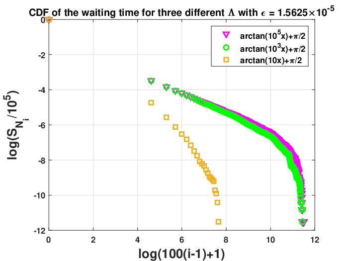
In this subsection, we test with three rate functions $\Lambda(x)$ which are inverse tangent functions with different stiffness. The three rate functions are

\Lambda_{1}(x)=\arctan(10^{5}x)+\frac{\pi}{2},\quad\Lambda_{2}(x)=\arctan(10^{3}x)+\frac{\pi}{2},\quad\Lambda_{3}(x)=\arctan(10x)+\frac{\pi}{2},

which are plotted in Fig.4. Clearly, $\Lambda_{1}$ has the sharpest transition from $0$ to $\pi$ , while $\Lambda_{2}$ increases less sharply and $\Lambda_{3}$ has the mildest transition. Besides, there is a positive lower bound $\frac{\pi}{2}$ when $x>0$ for all these three cases. However, we notice that these rate functions do not satisfy (2.4) since they do not strictly take $0$ value when $x<0$ , and their properties are beyond our theoretical analysis. But these rate functions ’morally’ satisfy the modeling principle as they are almost $0$ for $x<0$ up to a removal of a small neighborhood around $x=0$ . Thus, it is worth testing if these models also exhibit similar transitional behavior in terms of the waiting time distribution.

We take $\epsilon=1.5625\times 10^{-5}$ and run $10^{5}$ samples for the three different $\Lambda(x)$ . Similar as in subsection 5.3, $10^{5}$ waiting times $\{\tau^{n}\}_{n=1}^{10^{5}}$ as well as $\{N_{i}\}_{i=1}^{N_{t}}$ and $\{S_{N_{i}}\}_{i=1}^{N_{t}}$ are obtained for each $\Lambda(x)$ . We plot ( $\log(100(i-1)+1)$ , $\log[S_{N_{i}}/10^{5}]$ ) in Fig. 5 which is the CDF of the waiting time distribution in a log-log scale. As shown in Fig.5, the transition from a power-law decay to a more rapid decay is obvious when using $\Lambda_{1}(x)$ or $\Lambda_{2}(x)$ , but is less clear when using $\Lambda_{3}(x)$ . These results seem to suggest that (2.4) is not a necessary condition for the transitional behavior and a more comprehensive characterization calls for future studies.

6 Conclusion and discussions

In this work, we have explored the transitional behavior of the waiting time distribution of a state-dependent jump model, which may be interpreted as an underlying principle for the transitory anomalous diffusion at the macroscopic level.

The two approaches we have presented naturally complement each other. The asymptotic analysis leads to a fully specified description of the leading order behavior but its application is limited to a few cases. The probability method works for more generic parameter settings, but it only provides estimates in terms of the cumulative density functions, and there is no obvious way to justify the optimality of the derived bounds just by themselves. It is worth pointing out that, for simplicity of analysis, we have focused on the rate model (2.4) only to demonstrate the key components of the internal state causing the transitional phenomenon, but a series of rate models beyond Assumption (2.4) have been tested in our numerical experiments as well. And it is interesting to investigate in a more quantitative way how the transition rate affects the waiting time distribution and whether possible phase transitions exist.

This work also establishes a theoretical platform and a practical modeling methodology for incorporating transitional behavior in more complicated physical or biological systems. For example, we may study moving agents which have switching models with transitional waiting times in the future.

Acknowledgment

Z. X. and M. T are partially supported by NSFC 11871340, NSFC12031013, Shanghai pilot innovation project 21JC1403500. Y.Z. was supported by NSFC Tianyuan Fund for Mathematics grant, Project Number 12026606. Z.Z. has received support from the National Key R&D Program of China, Project Number 2021YFA1001200, 2020YFA0712000, and the NSFC grant, Project Number 12031013, 12171013.

Appendix A The introduction of the Kummer’s function

Kummer’s function of the first kind $M(a,b,z)$ is a solution of the confluent hyper-geometric differential equation

z\frac{d^{2}w}{dz^{2}}+(b-z)\frac{dw}{dz}-aw=0,

where $a$ , $b$ are two constant.

$M(a,b,z)$ has a hyper-geometric series given by

M(a,b,z)=1+\frac{a}{b}z+\frac{a(a+1)}{b(b+1)2!}z^{2}+...

(A.1)

We have

M(a,b,z)\to 1,\quad z\to 0.

(A.2)

When $z\to\infty$ , one gets

M(a,b,z)\sim e^{z}z^{a-b}\frac{\Gamma(b)}{\Gamma(a)},\quad|\mathbf{ph}z|<\frac{1}{2}\pi,

(A.3)

where $\mathbf{ph}z$ is the principle value of $a$ , $-\pi<\mathbf{ph}z<\pi$ and $a\neq 0,-1,-2...$ .

Appendix B The introduction of the parabolic cylinder functions

Parabolic cylinder functions are solutions of the differential equation

\frac{d^{2}y}{dx^{2}}+(a_{0}x^{2}+b_{0}x+c_{0})x=0,

which can be converted into the following form

\frac{d^{2}y}{dx^{2}}-(\frac{1}{4}x^{2}+a)y=0.

(B.1)

(B.1) has two standard solutions [1, 19]

	$\displaystyle U(a,x)$	$\displaystyle={}\frac{\sqrt{\pi}}{2^{\frac{a}{2}+\frac{1}{4}}\Gamma(\frac{3}{4}+\frac{a}{2})}e^{-\frac{\epsilon}{4}x^{2}}M\left(\frac{a}{2}+\frac{1}{4},\frac{1}{2},\frac{1}{2}x^{2}\right)$
		$\displaystyle-{}\frac{\sqrt{\pi}}{2^{\frac{a}{2}-\frac{1}{4}}\Gamma(\frac{1}{4}+\frac{a}{2})}xe^{-\frac{\epsilon}{4}x^{2}}M\left(\frac{a}{2}+\frac{3}{4},\frac{3}{2},\frac{1}{2}x^{2}\right).$		(B.2)

V(a,x)=\frac{\sin\left[\pi(\frac{1}{4}+\frac{a}{2})\right]Y_{1}+\cos\left[\pi(\frac{1}{4}+\frac{a}{2})\right]Y_{2}}{\Gamma(\frac{1}{2}-a)},

(B.3)

where

	$\displaystyle Y_{1}$	$\displaystyle={}\frac{1}{\sqrt{\pi}}\frac{\Gamma(\frac{1}{4}-\frac{a}{2})}{2^{\frac{a}{2}+\frac{1}{4}}}e^{-\frac{\epsilon}{4}x^{2}}M\left(\frac{a}{2}+\frac{1}{4},\frac{1}{2},\frac{1}{2}x^{2}\right),$
	$\displaystyle Y_{2}$	$\displaystyle={}\frac{1}{\sqrt{\pi}}\frac{\Gamma(\frac{3}{4}-\frac{a}{2})}{2^{\frac{a}{2}-\frac{1}{4}}}xe^{-\frac{\epsilon}{4}x^{2}}M\left(\frac{a}{2}+\frac{3}{4},\frac{3}{2},\frac{1}{2}x^{2}\right).$

Here, $M$ is the Kummer’s function in (A.1).

We have

U(a,x)\sim e^{-\frac{1}{4}x^{2}}x^{-a-\frac{1}{2}}\left[1+O(\frac{1}{x^{2}})\right],\quad x\to\infty,

(B.4)

V(a,x)\sim\sqrt{\frac{2}{\pi}}e^{\frac{1}{4}x^{2}}x^{a-\frac{1}{2}}\left[1+O(\frac{1}{x^{2}})\right],\quad x\to\infty.

(B.5)

and

\lim_{x\to 0+}U(a,x)=\frac{\sqrt{\pi}}{2^{\frac{a}{2}+\frac{1}{4}}\Gamma(\frac{3}{4}+\frac{a}{2})}.

(B.6)

For the derivative of $U(a,x)$ , one has[19]

U^{{}^{\prime}}(a,x)=\frac{1}{2}xU(a,x)-U(a-1,x),

(B.7)

and

\lim_{x\to 0+}U^{{}^{\prime}}(a,0+)=-\frac{\sqrt{\pi}}{2^{\frac{a}{2}-\frac{1}{4}}\Gamma(\frac{a}{2}+\frac{1}{4})}.

(B.8)

References

[1] M. Abramowitz, Handbook of mathematical functions, US Department of Commerce, 10 (1972).
[2] J.-P. Bouchaud and A. Georges, Anomalous diffusion in disordered media: statistical mechanisms, models and physical applications, Phys. Rep., 195 (1990), pp. 127–293.
[3] D. R. Cox, Renewal theory, methuen & co. ltd, 1962.
[4] E. Daly and A. Porporato, State-dependent fire models and related renewal processes, Phys. Rev. E, 74 (2006), p. 041112.
[5] E. Daly and A. Porporato, Intertime jump statistics of state-dependent poisson processes, Phys. Rev. E, 75 (2007), p. 011119.
[6] M. Dentz, A. Cortis, H. Scher, and B. Berkowitz, Time behavior of solute transport in heterogeneous media: transition from anomalous to normal transport, Advances in Water Resources, 27 (2004), pp. 155–173.
[7] A. Fick, Ueber diffusion, Annalen der Physik, 170 (1855), pp. 59–86, \urlhttps://doi.org/https://doi.org/10.1002/andp.18551700105, \urlhttps://onlinelibrary.wiley.com/doi/abs/10.1002/andp.18551700105.
[8] F. B. Hanson, Applied Stochastic Processes and Control for Jump-Diffusions: Modeling, Analysis and Computation, Society for Industrial and Applied Mathematics, Philadelphia, PA, 2007, \urlhttps://doi.org/10.1137/1.9780898718638, \urlhttps://epubs.siam.org/doi/abs/10.1137/1.9780898718638.
[9] J. W. Haus and K. W. Kehr, Diffusion in regular and disordered lattices, Phys. Rep., 150 (1987), pp. 263–406.
[10] O. Ibe, Markov processes for stochastic modeling, Newnes, 2013.
[11] N. Ikeda and S. Watanabe, Stochastic differential equations and diffusion processes, Elsevier, 2014.
[12] J.-H. Jeon, E. Barkai, and R. Metzler, Noisy continuous time random walks, The Journal of Chemical Physics, 139 (2013), p. 09B616_1.
[13] J. Klafter and G. Zumofen, Lévy statistics in a hamiltonian system, Phys. Rev. E, 49 (1994), pp. 4873–4877, \urlhttps://doi.org/10.1103/PhysRevE.49.4873, \urlhttps://link.aps.org/doi/10.1103/PhysRevE.49.4873.
[14] J.-G. Liu, Z. Wang, Y. Zhang, and Z. Zhou, Rigorous justification of the fokker–planck equations of neural networks based on an iteration perspective, SIAM J. Math. Anal., 54 (2022), pp. 1270–1312.
[15] R. Metzler, J.-H. Jeon, A. G. Cherstvy, and E. Barkai, Anomalous diffusion models and their properties: non-stationarity, non-ergodicity, and ageing at the centenary of single particle tracking, Phys. Chem. Chem. Phys., 16 (2014), pp. 24128–24164, \urlhttps://doi.org/10.1039/C4CP03465A, \urlhttp://dx.doi.org/10.1039/C4CP03465A.
[16] R. Metzler and J. Klafter, The random walk’s guide to anomalous diffusion: a fractional dynamics approach, Phys. Rep., 339 (2000), pp. 1–77.
[17] D. Molina-Garcia, T. Sandev, H. Safdari, G. Pagnini, A. Chechkin, and R. Metzler, Crossover from anomalous to normal diffusion: truncated power-law noise correlations and applications to dynamics in lipid bilayers, New J. Phys., 20 (2018), p. 103027.
[18] E. W. Montroll and G. H. Weiss, Random walks on lattices. ii, J. Math. Phys., 6 (1965), pp. 167–181.
[19] F. W. J. Olver, A. B. O. Daalhuis, D. W. Lozier, B. I. Schneider, R. F. Boisvert, C. W. Clark, B. R. Miller, B. V. Saunders, H. S. Cohl, and M. A. McClain, nist digital library of mathematical functions, \urlhttps://dlmf.nist.gov/.
[20] G. A. Pavliotis, Stochastic processes and applications: diffusion processes, the Fokker-Planck and Langevin equations, vol. 60, Springer, 2014.
[21] F. A. Reis and D. D. Caprio, Crossover from anomalous to normal diffusion in porous media, Phys. Rev. E, 89 (2014), p. 062126.
[22] H. Scher and E. W. Montroll, Anomalous transit-time dispersion in amorphous solids, Phys. Rev. B, 12 (1975), pp. 2455–2477, \urlhttps://doi.org/10.1103/PhysRevB.12.2455, \urlhttps://link.aps.org/doi/10.1103/PhysRevB.12.2455.
[23] J. R. Shoenfield, Markov a. a.. theory of algorithms, J. Symb. Log., 27 (1962), pp. 244–244, \urlhttps://doi.org/10.2307/2964158.
[24] Y. Tu and G. Grinstein, How white noise generates power-law switching in bacterial flagellar motors, Phys. Rev. Lett., 94 (2005), p. 208101.
[25] X. Xue, C. Xue, and M. Tang, The role of intracellular signaling in the stripe formation in engineered escherichia coli populations, PLoS computational biology, 14 (2018), p. e1006178.
[26] Z. Zhou, Y. Zhang, Y. Xie, Z. Wang, and J.-G. Liu, Investigating the integrate and fire model as the limit of a random discharge model: a stochastic analysis perspective, Mathematical Neuroscience and Applications, 1 (2021).

Transition behavior of the waiting time distribution in a jumping model with the internal state

Abstract

1 Introduction

2 The model and the main results

2.1 The model

The PDE model.

2.2 Main results

Proposition 2.1.

Theorem 2.1.

3 Asymptotic analysis of the PDE model

3.1 The explicit formula of n^​(s)\hat{n}(s)

Solve f^+​(x,s)\hat{f}_{+}(x,s).

Solve f^−\hat{f}_{-}.

Connecting f^+\hat{f}_{+} and f^−\hat{f}_{-}.

The explicit formula for n^​(s)\hat{n}(s).

3.2 The asymptotic approximation when s∼O⁡(1)s\sim O(1)

3.3 The asymptotic approximation when s=O⁡(ϵ2)s=O(\epsilon^{2})

4 The proof of Theorem 2.1

4.1 Exponential decay in the macroscopic time scale

Proposition 4.1.

Lemma 4.1.

Proof.

Remark 4.1.

Lemma 4.2.

Proof.

Lemma 4.3.

Proof.

Corollary 4.1.

Proof.

Lemma 4.4.

Proof.

Lemma 4.5.

Proof.

Lemma 4.6.

Proof.

Proof.

4.2 Power law decay in the mesoscopic time scale

Proposition 4.2.

Lemma 4.7.

Proof.

5 Numerical simulations

5.1 The algorithm

5.2 The case when ϵ=0\epsilon=0.

5.3 The case when ϵ≠0\epsilon\neq 0 and Λ\Lambda being piece-wise constant

5.4 Different ϵ\epsilon for Λ\Lambda being an inverse tangent function

6 Conclusion and discussions

Acknowledgment

Appendix A The introduction of the Kummer’s function

Appendix B The introduction of the parabolic cylinder functions

References

3.1 The explicit formula of $\hat{n}(s)$

Solve $\hat{f}_{+}(x,s)$ .

Solve $\hat{f}_{-}$ .

Connecting $\hat{f}_{+}$ and $\hat{f}_{-}$ .

The explicit formula for $\hat{n}(s)$ .

3.2 The asymptotic approximation when $s\sim O(1)$

3.3 The asymptotic approximation when $s=O(\epsilon^{2})$

5.2 The case when $\epsilon=0$ .

5.3 The case when $\epsilon\neq 0$ and $\Lambda$ being piece-wise constant

5.4 Different $\epsilon$ for $\Lambda$ being an inverse tangent function