跳到论文正文
W Papers独立论文阅读器 arXiv:2303.06778 论文正文 计算阅读时间 · 0%
引用这篇论文根据当前论文元数据生成,正式投稿前建议核对。


License: arXiv.org perpetual non-exclusive license
arXiv:2303.06778v2 [math.OC] 20 Jan 2024

Sublevel Set Approximation in The Hausdorff and Volume Metric with Application to Path Planning and Obstacle Avoidance

Morgan Jones Thanks: M. Jones is with the Department of Automatic Control and Systems Engineering, The University of Sheffield, Amy Johnson Building, Mappin Street, Sheffield, S1 3JD. e-mail: morgan.jones@sheffield.ac.uk
Abstract

Under what circumstances does the “closeness” of two functions imply the “closeness” of their respective sublevel sets? In this paper, we answer this question by showing that if a sequence of functions converges strictly from above/below to a function, VV, in the L∞L^{\infty} (or L1L^{1}) norm then these functions yield a sequence sublevel sets that converge to the sublevel set of VV with respect to the Hausdorff metric (or volume metric). Based on these theoretical results we propose Sum-of-Squares (SOS) numerical schemes for the optimal outer/inner polynomial sublevel set approximation of various sets, including intersections and unions of semialgebraic sets, Minkowski sums, Pontryagin differences and discrete points. We present several numerical examples demonstrating the usefulness of our proposed algorithm including approximating sets of discrete points to solve machine learning one-class classification problems and approximating Minkowski sums to construct C-spaces for computing optimal collision-free paths for Dubin’s car.

I Introduction

The notion of a set is a fundamental object of the modern mathematical toolkit, simply defined as a collection of elements. Sets are ubiquitous throughout control theory and are the language we use to represent frequently encountered concepts such as uncertainty [1, 2], regions of attraction [3, 4], reachable states [5, 6], invariant sets [7], attractors [8, 9], admissible inputs [10], feasible states [11], etc. Even for simple, low-dimensional problems, such sets can contain vast complexities and be numerically challenging to manipulate and analyze. As modern engineering systems become increasingly complex, we can expect that this problem will be exacerbated as the sets we encounter become ever more unwieldy. In this context, we present several fundamental results for the approximation of sets, along with associated implementable numerical schemes based on Sum-of-Squares (SOS) programming.

For some given set X⊂ℝnX\subset\mathbb{R}^{n}, the goal of this paper is to find an outer or inner set approximation of XX. Specifically, we would like to compute another set Y⊂ℝnY\subset\mathbb{R}^{n} such that X⊆YX\subseteq Y (outer approximation) or Y⊆XY\subseteq X (inner approximation) and Y≈XY\approx X, where the approximation is defined with respect to some set metric.

Previous attempts at solving this set approximation problem were based on the fact that the volume of an ellipsoid, {x∈ℝn:x⊤​A​x<0}\{x\in\mathbb{R}^{n}:x^{\top}Ax<0\}, is proportional to det(A−1)\det(A^{-1}). Then an equivalent optimization problem can be constructed for computing outer ellipsoid approximations by minimizing the convex objective function −logdet(A)-\log\det(A) [12]. This approach of determinant maximization has been heuristically generalized to the problem of computing outer SOS polynomial sublevel approximations [13, 14]. Alternative heuristic matrix trace maximization schemes have also been proposed [15]. The seminal work of [16] solved the related problem of approximating an integral over a semialgebraic set using the moment approach, showing that the dual to this problem can give outer semialgebraic set approximations.

More recently, in the special case of star convex semialgebraic sets, a heuristic approach based on sublevel set scaling has been proposed in [17], demonstrating impressive numerical set approximation results based on SOS programming. An approach based on L1L^{1} maximization, similar to some of the schemes proposed in this paper, has been proposed in [18, 19]. However, the work of [18] only considers the specific problem of approximating Pontryagin differences and lacks convergence guarantees and [19] only considers the specific problem of approximating semialgebraic in the volume metric. In [20] sets defined by quantifiers are approximated in the volume metric to arbitrary accuracy. In this paper we extend [20] to the volume metric approximation of more general sets, represented as sublevel sets of integrable functions. Moreover, we propose a new fundamental result for the approximation sets in the Hausdorff metric. Other works that have dealt with the problem of set approximation in the Hausdorff metric include the excellent work of [21] that considered the problem of mollifying feasible constraints and helped to inspire the proof of the Hausdorff set approximations in this paper.

The main contributions of this paper is to show that when X⊂ℝnX\subset\mathbb{R}^{n} can be written as a sublevel set of some function VV over a compact set (or only finite Lebesgue measurable in the case of volume approximation) Λ⊂ℝn\Lambda\subset\mathbb{R}^{n}. the following holds:

  • •

    Approximating VV in the L∞L^{\infty} norm from above by some function JJ yields a sublevel set Y={x∈Λ:J⁡(x)<γ}Y=\{x\in\Lambda:J(x)<\gamma\} that provides an arbitrarily accurate inner approximation of XX in the Hausdorff metric.

  • •

    Approximating VV in the L1L^{1} norm from above by some function JJ yields a sublevel set Y={x∈Λ:J⁡(x)<γ}Y=\{x\in\Lambda:J(x)<\gamma\} that provides an arbitrarily accurate inner approximation of XX in the volume metric.

The above sublevel set approximation results provide us with guiding principles for the design of numerical procedures for set approximation. Firstly, given a set, XX, we must write XX as a sublevel set of some function VV. Fortunately, this requirement is not difficult to satisfy for many of the sets encountered in control theory and in this work we demonstrate this by presenting VV explicitly for intersections and unions of semialgebraic sets, Minkowski sums, Pontryagin differences and discrete points. Although not considered in this work, our framework can still be applied when VV is not known explicitly, rather it is implicitly defined such as when VV is a Lyapunov function [3] or value function [6]. After finding VV, we must find a function JJ that minimizes ‖V−J‖||V-J|| such that V⁡(x)≤J⁡(x)V(x)\leq J(x), where ||⋅||||\cdot|| is the L1L^{1} or L∞L^{\infty} norm. By introducing auxiliary variables we show that this optimization problem can be lifted to a convex optimization problem and solved by tightening the inequality constraints to SOS constraints for many set approximation problems with Volume/Hausdorff metric convergence guarantees.

To summarize our contribution, to the best of the authors knowledge, only the works of [19, 20] provide numerical schemes with volume metric convergence guarantees for the approximation semialgebraic sets and sets defined by quantifiers respectively. In contrast our work expands on these ideas and provides numerical schemes with convergence guarantees in both the Hausdorff and volume metric for a larger class of sets such as unions of semialgebraic sets, Minkowski sums, Pontryagin differences and discrete points. Moreover, the main results of the paper, stated in Theorems 1 and 2, are independent of SOS programming, allowing exploration of alternative numerical schemes such as those found in [22].

I-A Application to Path Planning and Obstacle Avoidance

The path planning of autonomous systems is the computational problem of finding the sequence of inputs that moves a given object from an initial condition to a target set while avoiding obstacles. Computing optimal paths is a well researched subject, with a broad range of practical uses ranging from the navigation of UAVs [23] to the precise movements of robotic manipulators [24].

Many popular algorithms for solving the path planning problem, such as A∗A^{*} or Dijkstra, do not inherently account for the size and shape of the object that travels along the path. A common method for overcoming this problem is to transform the workspace of the problem to a Configuration-space (C-space), where in C-space the object is represented by a single point and obstacles are enlarged to account for the loss of size and shape of the object. The enlarged obstacles in C-space are given by the Minkowski sum of the sets representing the object and obstacles. In special convex cases the Minkowski sum can be found as a closed form solution [25], however, unfortunately there is no analytical expression for the Minkowski sum of two general sets. In the absence of an analytical expression for Minkowski sums we rely on numerical approximations. Numerical schemes have previously been proposed for the case of ellipsoid objects and convex objects [26] and also for more general sets using SOS and logdet\log\det heuristics [27]. In this paper we apply our proposed SOS based numerical scheme for set approximation, with convergence guarantees, to the problem of approximating Minkowski sums in order to construct C-spaces.

II Notation

For A⊂ℝnA\subset\mathbb{R}^{n} we denote the indicator function by 𝟙A:ℝn→ℝ\mathds{1}_{A}:\mathbb{R}^{n}\to\mathbb{R} that is defined as 𝟙A​(x)={1​ if ​x∈A0​ otherwise.\mathds{1}_{A}(x)=\begin{cases}&1\text{ if }x\in A\\ &0\text{ otherwise.}\end{cases} For B⊆ℝnB\subseteq\mathbb{R}^{n}, μ⁡(B):=∫ℝn𝟙B​(x)​𝑑x\mu(B):=\int_{\mathbb{R}^{n}}\mathds{1}_{B}(x)dx is the Lebesgue measure of BB. We denote the Hausdorff metric (given in Eq. (3)) by DHD_{H} and the volume metric (given in Eq. (8)) by DVD_{V}. For two sets A,B∈ℝnA,B\in\mathbb{R}^{n} we denote A/B={x∈A:x∉B}A/B=\{x\in A:x\notin B\}. For x∈ℝnx\in\mathbb{R}^{n} we denote ‖x‖p=(∑i=1nxip)1p||x||_{p}=\left(\sum_{i=1}^{n}x_{i}^{p}\right)^{\frac{1}{p}}. For η>0\eta>0 and y∈ℝny\in\mathbb{R}^{n} we denote the set Bη​(y)={x∈ℝn:‖x−y‖2<η}B_{\eta}(y)=\{x\in\mathbb{R}^{n}:||x-y||_{2}<\eta\}. We say f:Ω→ℝf:\Omega\to\mathbb{R} is such that f∈L1​(Ω,ℝ)f\in L^{1}(\Omega,\mathbb{R}) if ‖f‖L1​(Ω,ℝ):=∫Ω|f⁡(x)|​𝑑x<∞||f||_{L^{1}(\Omega,\mathbb{R})}:=\int_{\Omega}|f(x)|dx<\infty. We define the L∞L^{\infty} norm as ‖f‖L∞​(Ω,ℝ):=supx∈Ω|f⁡(x)|||f||_{L^{\infty}(\Omega,\mathbb{R})}:=\sup_{x\in\Omega}|f(x)|. We denote the space of polynomials p:ℝn→ℝp:\mathbb{R}^{n}\to\mathbb{R} by ℝ⁡[x]\mathbb{R}[x] and polynomials with degree at most d∈ℕd\in\mathbb{N} by ℝd​[x]\mathbb{R}_{d}[x]. We say p∈ℝ2​d​[x]p\in\mathbb{R}_{2d}[x] is Sum-of-Squares (SOS) if there exists pi∈ℝd​[x]p_{i}\in\mathbb{R}_{d}[x] such that p⁡(x)=∑i=1k(pi​(x))2p(x)=\sum_{i=1}^{k}(p_{i}(x))^{2}. We denote ∑S​O​Sd\sum_{SOS}^{d} to be the set of SOS polynomials of at most degree d∈ℕd\in\mathbb{N} and the set of all SOS polynomials as ∑S​O​S\sum_{SOS}. For two sets A,B⊂ℝnA,B\subset\mathbb{R}^{n} we denote the Minkowski sum by A⊕BA\oplus B (defined in Eq. (29)) and Pontryagin difference by A⊖BA\ominus B (defined in Eq. (34)). If MM is a subspace of a vector space XX we denote equivalence relation ∼M\sim_{M} for x,y∈Xx,y\in X by x∼Myx\sim_{M}y if x−y∈Mx-y\in M. We denote quotient space by X(modM):={{y∈X:y∼Mx}:x∈X}X\pmod{M}:=\{\{y\in X:y\sim_{M}x\}:x\in X\}.

III Sublevel Set Approximation

Given a set X⊂ℝnX\subset\mathbb{R}^{n}, the goal of this paper is to solve he following problem,

Y∗∈arginfY∈𝒞DS(X,Y),\displaystyle Y^{*}\in\arg\inf_{Y\in\mathcal{C}}D_{S}(X,Y), (1)

where DSD_{S} is some set metric providing a notion of how close set Y∗Y^{*} is to XX and 𝒞\mathcal{C} is some set of feasible sets.

The decision variables in Opt. (1) are sets, which are uncountable objects. This poses a challenge as it is difficult to search and hence optimize over sets effectively. To make such set optimization problems tractable, we need to find ways to parameterize our decision variables. The approach we take to overcome this problem is to consider problems where both our target set, XX, and our decision variable, YY, are sublevel sets of functions, taking the following forms X={x∈Λ:V⁡(x)<γ}X=\{x\in\Lambda:V(x)<\gamma\} and Y={x∈Λ:J⁡(x)<γ}Y=\{x\in\Lambda:J(x)<\gamma\}, where Λ⊂ℝn\Lambda\subset\mathbb{R}^{n} and γ∈ℝ\gamma\in\mathbb{R}. Then, rather than attempting to directly solve the “geometric” set optimiziation problem in Eq (1), we consider the following associated “algebriac” optimization problem,

J∗∈arginfJ∈ℱDF(V,J),\displaystyle J^{*}\in\arg\inf_{J\in\mathcal{F}}D_{F}(V,J), (2)

where DFD_{F} is some function metric providing a notion of the distance between the functions VV and JJ and ℱ\mathcal{F} is some finite dimensional function space.

The decision variables of Opt. (2) are functions and hence can be easily optimized over by parametrizing the decision variables using basis functions. We next turn our attention to the question of when does solving Opt. (2) yield a close solution to Opt. (1)? More specifically, if X={x∈Λ:V⁡(x)<γ}X=\{x\in\Lambda:V(x)<\gamma\}, Y={x∈Λ:J⁡(x)<γ}Y=\{x\in\Lambda:J(x)<\gamma\} and J≈VJ\approx V when is it true that X≈YX\approx Y? In the following subsections we answer this question by showing that, for a given function, V:ℝn→ℝV:\mathbb{R}^{n}\to\mathbb{R}, a compact set, Λ⊂ℝn\Lambda\subset\mathbb{R}^{n}, and a sequence of functions, {Jd}d∈ℕ\{J_{d}\}_{d\in\mathbb{N}}, the following hold:

  1. (A)

    If Jd​(x)≥V⁡(x)J_{d}(x)\geq V(x) for all x∈Λx\in\Lambda and Jd→VJ_{d}\to V as d→∞d\to\infty in the L∞​(Λ,ℝn)L^{\infty}(\Lambda,\mathbb{R}^{n}) norm then for any γ>0\gamma>0 we have that {x∈Λ:Jd​(x)<γ}→{x∈Λ:V⁡(x)<γ}\{x\in\Lambda:J_{d}(x)<\gamma\}\to\{x\in\Lambda:V(x)<\gamma\} with respect to the Hausdorff metric (defined in Eq. (3)).

  2. (B)

    If V​(x)≤Jd​(x)V(x)\leq J_{d}(x) for all x∈Λx\in\Lambda and Jd→VJ_{d}\to V as d→∞d\to\infty in the L1​(Λ,ℝn)L^{1}(\Lambda,\mathbb{R}^{n}) norm then for any γ>0\gamma>0 we have that {x∈Λ:Jd​(x)<γ}→{x∈Λ:V⁡(x)<γ}\{x\in\Lambda:J_{d}(x)<\gamma\}\to\{x\in\Lambda:V(x)<\gamma\} in the volume metric (defined in Eq. (8)).

III-A Sublevel Set Approximation In The Hausdorff Metric

For sets A,B⊂ℝnA,B\subset\mathbb{R}^{n}, we denote the Hausdorff metric as DH​(A,B)D_{H}(A,B), defining

DH​(A,B):=max⁡{H⁡(A,B),H⁡(B,A)},\qquad\qquad D_{H}(A,B):=\max\{H(A,B),H(B,A)\}, (3)

where H⁡(A,B):=supx∈AD⁡(x,B)H(A,B):=\sup_{x\in A}D(x,B) and D⁡(x,B):=infy∈B{∥x−y∥2}D(x,B):=\inf_{y\in B}\{\lVert{x-y}\rVert_{2}\}.

We now show that uniform convergence of functions yields sublevel approximation in the Hausdorff metric.

Theorem 1.

Consider a compact set Λ⊂ℝn\Lambda\subset\mathbb{R}^{n}, a function V:Λ→ℝV:\Lambda\to\mathbb{R}, and a family of functions {Jd}d∈ℕ\{J_{d}\}_{d\in\mathbb{N}} that satisfies the following properties:

  1. 1.

    For any d∈ℕd\in\mathbb{N} we have V​(x)≤Jd​(x)V(x)\leq J_{d}(x) for all x∈Λx\in\Lambda.

  2. 2.

    limd→∞supx∈Λ|V⁡(x)−Jd​(x)|=0\lim_{d\to\infty}\sup_{x\in\Lambda}|V(x)-J_{d}(x)|=0.

Then for all γ∈ℝ\gamma\in\mathbb{R} we have that,

limd→∞DH​({x∈Λ:Jd​(x)<γ},{x∈Λ:V⁡(x)<γ})=0.\displaystyle\lim_{d\to\infty}D_{H}\bigg(\{x\in\Lambda:J_{d}(x)<\gamma\},\{x\in\Lambda:V(x)<\gamma\}\bigg)=0. (4)
Proof.

Throughout this proof we use the following notation Xd:={x∈Λ:Jd​(x)<γ}X_{d}:=\{x\in\Lambda:J_{d}(x)<\gamma\} and X∗:={x∈Λ:V⁡(x)<γ}X^{*}:=\{x\in\Lambda:V(x)<\gamma\}.

Now, recall from Eq. (3) that the Hausdorff metric for two sets Xd,X∗⊂ℝnX_{d},X^{*}\subset\mathbb{R}^{n} is defined as the maximum of two terms, DH​(Xd,X∗):=max⁡{H⁡(Xd,X∗),H⁡(X∗,Xd)}D_{H}(X_{d},X^{*}):=\max\{H(X_{d},X^{*}),H(X^{*},X_{d})\}, where H⁡(Xd,X∗):=supx∈XdD⁡(x,X∗)H(X_{d},X^{*}):=\sup_{x\in X_{d}}D(x,X^{*}) and D⁡(x,X∗):=infy∈X∗{∥x−y∥2}D(x,X^{*}):=\inf_{y\in X^{*}}\{\lVert{x-y}\rVert_{2}\}. This naturally leads us to split the remainder of the proof into two parts. In Part 1 of the proof we show that the first term is such that H⁡(Xd,X∗)=0H(X_{d},X^{*})=0 for all d∈ℕd\in\mathbb{N}. In Part 2 of the proof we show that for all ε>0\varepsilon>0 there exists N∈ℕN\in\mathbb{N} such that for all d>Nd>N the second term is such that H⁡(X∗,Xd)<εH(X^{*},X_{d})<\varepsilon. Then Parts 1 and 2 of the proof can be used together to show Eq. (4), completing the proof.

Part 1 of proof: In this part of the proof we show H⁡(Xd,X∗)=0H(X_{d},X^{*})=0 for all d∈ℕd\in\mathbb{N}. Since V​(x)≤Jd​(x)V(x)\leq J_{d}(x) for all x∈Λx\in\Lambda it follows that Xd⊆X∗X_{d}\subseteq X^{*} for any d∈ℕd\in\mathbb{N}. Thus for all d∈ℕd\in\mathbb{N} and x∈Xdx\in X_{d} we have that D⁡(x,X∗)=0D(x,X^{*})=0. Therefore it clearly follows H⁡(Xd,X∗)=supx∈XdD⁡(x,X∗)=0H(X_{d},X^{*})=\sup_{x\in X_{d}}D(x,X^{*})=0 for all d∈ℕd\in\mathbb{N}.

Part 2 of proof: In this part of the proof we show that for all ε>0\varepsilon>0 there exists N∈ℕN\in\mathbb{N} such that for all d>Nd>N we have H⁡(X∗,Xd)<εH(X^{*},X_{d})<\varepsilon. For contradiction suppose the negation, that there exists δ>0\delta>0 such that

H⁡(X∗,Xd)>δ​ for all ​d∈ℕ.\displaystyle H(X^{*},X_{d})>\delta\text{ for all }d\in\mathbb{N}.

Then for each d∈ℕd\in\mathbb{N} there exists xd∈X∗x_{d}\in X^{*} such that

D⁡(xd,Xd)≥δ​ for all ​d∈ℕ.\displaystyle D(x_{d},X_{d})\geq\delta\text{ for all }d\in\mathbb{N}. (5)

Now, Xd⊆ΛX_{d}\subseteq\Lambda and Λ\Lambda is compact. Therefore the sequence {xd}d∈ℕ⊆Λ\{x_{d}\}_{d\in\mathbb{N}}\subseteq\Lambda is bounded. Thus, by the Bolzano Weierstrass Theorem (Thm. 7 found in Appendix VIII-D), there exists a convergent subsequence {yn}n∈ℕ⊆{xd}d∈ℕ\{y_{n}\}_{n\in\mathbb{N}}\subseteq\{x_{d}\}_{d\in\mathbb{N}}. Let us denote the limit point of {yn}n∈ℕ\{y_{n}\}_{n\in\mathbb{N}} by y∗∈Λy^{*}\in\Lambda.

Since {xd}d∈ℕ\{x_{d}\}_{d\in\mathbb{N}} satisfies Eq. (5) and {yn}n∈ℕ⊆{xd}d∈ℕ\{y_{n}\}_{n\in\mathbb{N}}\subseteq\{x_{d}\}_{d\in\mathbb{N}} it follows

D⁡(yn,Xn)≥δ​ for all ​n∈ℕ.\displaystyle D(y_{n},X_{n})\geq\delta\text{ for all }n\in\mathbb{N}. (6)

Moreover, because xd∈X∗x_{d}\in X^{*} for all d∈ℕd\in\mathbb{N} and {yn}n∈ℕ⊆{xd}d∈ℕ\{y_{n}\}_{n\in\mathbb{N}}\subseteq\{x_{d}\}_{d\in\mathbb{N}} it follows yn∈X∗y_{n}\in X^{*} for all n∈ℕn\in\mathbb{N}. Hence, εn:=γ−V⁡(yn)>0\varepsilon_{n}:=\gamma-V(y_{n})>0 for all n∈ℕn\in\mathbb{N}.

On the other hand, since limd→∞supx∈Λ|V⁡(x)−Jd​(x)|=0\lim_{d\to\infty}\sup_{x\in\Lambda}|V(x)-J_{d}(x)|=0 it follows for each n∈ℕn\in\mathbb{N} there exists Nn∈ℕN_{n}\in\mathbb{N} such that

Jd​(yn)−V⁡(yn)<εn​ for all ​d>Nn.\displaystyle J_{d}(y_{n})-V(y_{n})<\varepsilon_{n}\text{ for all }d>N_{n}. (7)

Since εn:=γ−V⁡(yn)>0\varepsilon_{n}:=\gamma-V(y_{n})>0, it follows by Eq. (7) that

Jd​(yn)<γ​ for all ​d>Nn,\displaystyle J_{d}(y_{n})<\gamma\text{ for all }d>N_{n},

which implies yn∈Xdy_{n}\in X_{d} for all d>Nnd>N_{n}.

Now, since yn→y∗y_{n}\to y^{*} there exists N∈ℕN\in\mathbb{N} such that ‖yn−y∗‖2<δ/4||y_{n}-y^{*}||_{2}<\delta/4 for all n>Nn>N. Fixing n>Nn>N and selecting d>max⁡{N,Nn}d>\max\{N,N_{n}\} (as in Eq. (7) so yn∈Xdy_{n}\in X_{d} for d>Nnd>N_{n}) we have that

D⁡(yd,Xd)=infx∈Xd‖yd−x‖2\displaystyle D(y_{d},X_{d})=\inf_{x\in X_{d}}||y_{d}-x||_{2}
≤‖yd−yn‖2≤||yd−y∗||2+‖yn−y∗‖2≤δ/2,\displaystyle\qquad\leq||y_{d}-y_{n}||_{2}\leq||y_{d}-y^{*}||_{2}+||y_{n}-y^{*}||_{2}\leq\delta/2,

contradicting Eq. (6). Thus it follows that for all ε>0\varepsilon>0 there exists N∈ℕN\hskip-1.42271pt\in\hskip-1.42271pt\mathbb{N} such that for all d>Nd>N we have H⁡(X∗,Xd)<εH(X^{*},X_{d})<\varepsilon. ∎

Remark 1.

The conditions that Λ\Lambda is compact, sublevel sets are strictly defined, V​(x)≤Jd​(x)V(x)\leq J_{d}(x) and limd→∞supx∈Λ|V⁡(x)−Jd​(x)|=0\lim_{d\to\infty}\sup_{x\in\Lambda}|V(x)-J_{d}(x)|=0 in Thm. 1 cannot be relaxed. In Section VIII-B we have presented several counterexamples showing that if any of these conditions are relaxed then it is not necessarily true that the sublevel sets of JdJ_{d} converge to the sublevel set of VV in the Hausdorff metric.

III-B Sublevel Set Approximation in The Volume Metric

For Lebesgue measurable sets A,B⊂ℝnA,B\subset\mathbb{R}^{n}, we denote the volume metric as DV​(A,B)D_{V}(A,B), where

DV​(A,B):=μ⁡((A/B)∪(B/A)),\qquad\qquad D_{V}(A,B):=\mu\bigg((A/B)\cup(B/A)\bigg), (8)

recalling from Sec. II that we denote μ⁡(A)\mu(A) as the Lebesgue measure of the set A⊂ℝnA\subset\mathbb{R}^{n}.

Theorem 2.

Consider a Lebesgue measurable set Λ⊂ℝn\Lambda\subset\mathbb{R}^{n} with finite Lebesgue measure, a function V∈L1​(Λ,ℝ)V\in L^{1}(\Lambda,\mathbb{R}), and a family of functions {Jd∈L1​(Λ,ℝ):d∈ℕ}\{J_{d}\in L^{1}(\Lambda,\mathbb{R}):d\in\mathbb{N}\} that satisfies the following properties:

  1. 1.

    For any d∈ℕd\in\mathbb{N} we have V​(x)≤Jd​(x)V(x)\leq J_{d}(x) for all x∈Λx\in\Lambda.

  2. 2.

    limd→∞‖V−Jd‖L1​(Λ,ℝ)=0\lim_{d\to\infty}||V-J_{d}||_{L^{1}(\Lambda,\mathbb{R})}=0.

Then for all γ∈ℝ\gamma\in\mathbb{R} we have that

limd→∞DV​({x∈Λ:Jd​(x)<γ},{x∈Λ:V⁡(x)<γ})=0.\displaystyle\lim_{d\to\infty}D_{V}\bigg(\{x\in\Lambda:J_{d}(x)<\gamma\},\{x\in\Lambda:V(x)<\gamma\}\bigg)=0. (9)
Proof.

Let us denote V~​(x)=−V​(x)\tilde{V}(x)=-V(x) and J~d​(x)=−Jd​(x)\tilde{J}_{d}(x)=-J_{d}(x). It follows that J~d​(x)≤V~​(x)\tilde{J}_{d}(x)\leq\tilde{V}(x) for all x∈Λx\in\Lambda and limd→∞‖V~−J~d‖L1​(Λ,ℝ)=0\lim_{d\to\infty}||\tilde{V}-\tilde{J}_{d}||_{L^{1}(\Lambda,\mathbb{R})}=0. Therefore, by Prop. 1 (found in the appendix) it follows that for any γ∈ℝ\gamma\in\mathbb{R} we have that,

limd→∞DV​({x∈Λ:V~​(x)≤γ},{x∈Λ:J~d​(x)≤γ})=0.\displaystyle\lim_{d\to\infty}D_{V}\bigg(\{x\in\Lambda:\tilde{V}(x)\leq\gamma\},\{x\in\Lambda:\tilde{J}_{d}(x)\leq\gamma\}\bigg)=0. (10)

Now, Λ={x∈Λ:V⁡(x)<γ}∪{x∈Λ:V⁡(x)≥γ}={x∈Λ:V⁡(x)<γ}∪{x∈Λ:V~​(x)≤−γ}\Lambda=\{x\in\Lambda:V(x)<\gamma\}\cup\{x\in\Lambda:V(x)\geq\gamma\}=\{x\in\Lambda:V(x)<\gamma\}\cup\{x\in\Lambda:\tilde{V}(x)\leq-\gamma\}. Therefore

{x∈Λ:V~​(x)≤−γ}=Λ/{x∈Λ:V⁡(x)<γ},\displaystyle\{x\in\Lambda:\tilde{V}(x)\leq-\gamma\}=\Lambda/\{x\in\Lambda:V(x)<\gamma\}, (11)

and by a similar argument

{x∈Λ:J~d​(x)≤−γ}=Λ/{x∈Λ:Jd​(x)<γ}.\displaystyle\{x\in\Lambda:\tilde{J}_{d}(x)\leq-\gamma\}=\Lambda/\{x\in\Lambda:J_{d}(x)<\gamma\}. (12)

Moreover, V​(x)≤Jd​(x)V(x)\leq J_{d}(x) it follows

{x∈Λ:V⁡(x)<γ}⊆{x∈Λ:Jd​(x)<γ},\displaystyle\{x\in\Lambda:V(x)<\gamma\}\subseteq\{x\in\Lambda:J_{d}(x)<\gamma\}, (13)

and hence

Λ/{x∈Λ:Jd​(x)<γ}⊆Λ/{x∈Λ:V⁡(x)<γ},\displaystyle\Lambda/\{x\in\Lambda:J_{d}(x)<\gamma\}\subseteq\Lambda/\{x\in\Lambda:V(x)<\gamma\}, (14)

Thus, by Lem. 7 (found in the appendix) and Eqs (11) (12) (13) (14) , we have that

DV​({x∈Λ:V⁡(x)<γ},{x∈Λ:Jd​(x)<γ})\displaystyle D_{V}\bigg(\{x\in\Lambda:V(x)<\gamma\},\{x\in\Lambda:J_{d}(x)<\gamma\}\bigg) (15)
=μ⁡({x∈Λ:V⁡(x)<γ})−μ⁡({x∈Λ:Jd​(x)<γ})\displaystyle=\mu(\{x\in\Lambda:V(x)<\gamma\})-\mu(\{x\in\Lambda:J_{d}(x)<\gamma\})
=(μ⁡(Λ)−μ⁡({x∈Λ:Jd​(x)<γ}))\displaystyle=\bigg(\mu(\Lambda)-\mu(\{x\in\Lambda:J_{d}(x)<\gamma\})\bigg)
−(μ⁡(Λ)−μ⁡({x∈Λ:V⁡(x)<γ}))\displaystyle\qquad-\bigg(\mu(\Lambda)-\mu(\{x\in\Lambda:V(x)<\gamma\})\bigg)
=μ⁡(Λ/{x∈Λ:Jd​(x)<γ})−μ⁡(Λ/{x∈Λ:V⁡(x)<γ})\displaystyle=\mu(\Lambda/\{x\in\Lambda:{J}_{d}(x)<\gamma\})-\mu(\Lambda/\{x\in\Lambda:{V}(x)<\gamma\})
=DV​(Λ/{x∈Λ:V⁡(x)<γ},Λ/{x∈Λ:Jd​(x)<γ})\displaystyle=D_{V}\bigg(\Lambda/\{x\in\Lambda:{V}(x)<\gamma\},\Lambda/\{x\in\Lambda:{J}_{d}(x)<\gamma\}\bigg)
=DV​({x∈Λ:V~​(x)≤−γ},{x∈Λ:J~d​(x)≤−γ}).\displaystyle=D_{V}\bigg(\{x\in\Lambda:\tilde{V}(x)\leq-\gamma\},\{x\in\Lambda:\tilde{J}_{d}(x)\leq-\gamma\}\bigg).

Now by Eqs (10) and (15) it follows that Eq. (9) holds. ∎

IV Numerical Sublevel Set Approximation

Given some set X⊂ℝnX\subset\mathbb{R}^{n} we would like to approximate, Theorems 1 and 2 illuminate the following steps we must take:

  1. 1.

    Write the set XX as a sublevel set of some function VV.

  2. 2.

    Approximate the function VV by a uniformly bounding function in the L∞L^{\infty} norm or L1L^{1} norm (depending on whether or not the set approximation is required to be with respect to the Hausdorff or volume metric).

Step 1 is always viable since by Prop. 4 (found in the appendix), it follows that for any compact set X⊂ℝnX\subset\mathbb{R}^{n} there always exists a smooth function VV such that X={x∈ℝn:V⁡(x)≤0}X=\{x\in\mathbb{R}^{n}:V(x)\leq 0\}. Sometimes it is possible to complete Step 2 when VV is not known analytically, such as for value functions [6] or Lyapunov functions [3]. However, for numerical implementation in this work we will only consider cases where VV is known explicitly. Later, in the following subsections, we will present several analytical expressions of VV for various classes of sets including intersections and unions of semialgebraic sets, Minkowski sums, Pontryagin differences and discrete points. Before proceeding to these subsections we next briefly discuss the general approach we take to solving Step 2, approximating VV by a uniformly bounding function in either the L∞L^{\infty} or L1L^{1} norm.

An optimization problem for L∞L^{\infty} approximation

For a given function VV let us consider the problem of approximating VV uniformly from above in the L∞L^{\infty} norm,

Jd∗∈\displaystyle J_{d}^{*}\in arginfJd∈ℝd​[x]supx∈Λ|V(x)−Jd(x)|\displaystyle\arg\inf_{J_{d}\in\mathbb{R}_{d}[x]}\sup_{x\in\Lambda}|V(x)-J_{d}(x)| (16)
such that ​V​(x)≤Jd​(x)​ for all ​x∈Λ.\displaystyle\text{such that }V(x)\leq J_{d}(x)\text{ for all }x\in\Lambda.

Unfortunately, Opt. (16) is a bi-level optimization problem, having a nested supremum inside the objective function. This makes the problem challenging to solve as our numerical implementation is based on SOS programming (although alternatives to SOS exist [22]) that requires the coefficients of the polynomial decision variable, Jd∈ℝd​[x]J_{d}\in\mathbb{R}_{d}[x], to appear linearly in the objective function. Fortunately, it is possible to lift the problem to a convex problem, where all unknown coefficients appear linearly in the constraints and objective function, by introducing extra decision variables in the following way,

Jd∗∈\displaystyle J_{d}^{*}\in arginfJd∈ℝd​[x],Pd∈ℝd​[x],γ∈ℝγ\displaystyle\arg\inf_{J_{d}\in\mathbb{R}_{d}[x],P_{d}\in\mathbb{R}_{d}[x],\gamma\in\mathbb{R}}\gamma (17)
such that ​Pd​(x)≤V⁡(x)≤Jd​(x)​ for all ​x∈Λ,\displaystyle\text{such that }P_{d}(x)\leq V(x)\leq J_{d}(x)\text{ for all }x\in\Lambda,
Jd​(x)−Pd​(x)<γ​ for all ​x∈Λ.\displaystyle\hskip 42.67912ptJ_{d}(x)-P_{d}(x)<\gamma\text{ for all }x\in\Lambda.

An optimization problem for L1L^{1} approximation

For a given function VV let us consider the problem of approximating VV uniformly from above in the L1L^{1} norm,

Jd∗∈\displaystyle J_{d}^{*}\in argsupJd∈ℝd​[x]∫Λ|Jd(x)−V(x)|dx\displaystyle\arg\sup_{J_{d}\in\mathbb{R}_{d}[x]}\int_{\Lambda}|J_{d}(x)-V(x)|dx (18)
such that ​V​(x)≤Jd​(x)​ for all ​x∈Λ.\displaystyle\text{such that }V(x)\leq J_{d}(x)\text{ for all }x\in\Lambda.

Since the constraints of Opt. (18) enforce V​(x)≤Jd​(x)V(x)\leq J_{d}(x) it follows that ∫Λ|Jd​(x)−V⁡(x)|𝑑x=∫ΛJd​(x)​𝑑x−∫ΛV⁡(x)​𝑑x\int_{\Lambda}|J_{d}(x)-V(x)|dx=\int_{\Lambda}J_{d}(x)dx-\int_{\Lambda}V(x)dx. Since ∫ΛV⁡(x)​𝑑x\int_{\Lambda}V(x)dx is a constant it is equivalent to minimize ∫ΛJd​(x)​𝑑x\int_{\Lambda}J_{d}(x)dx as it is to minimize ∫Λ|Jd​(x)−V⁡(x)|​𝑑x\int_{\Lambda}|J_{d}(x)-V(x)|dx. Hence, rather than solving Opt. (18) we solve,

Jd∗∈\displaystyle J_{d}^{*}\in arginfJd∈ℝd​[x]∫ΛJd(x)dx\displaystyle\arg\inf_{J_{d}\in\mathbb{R}_{d}[x]}\int_{\Lambda}J_{d}(x)dx (19)
such that ​V​(x)≤Jd​(x)​ for all ​x∈Λ.\displaystyle\text{such that }V(x)\leq J_{d}(x)\text{ for all }x\in\Lambda.

Interestingly, Opt. (19) shares some similarities to the dual problem in [16] for the approximation of integrals over sets.

It is also useful to consider a similar optimization problem to Opt. (19) that yields outer sublevel set approximations

Jd∗∈\displaystyle J_{d}^{*}\in argsupJd∈ℝd​[x]∫ΛJ(x)dx\displaystyle\arg\sup_{J_{d}\in\mathbb{R}_{d}[x]}\int_{\Lambda}J(x)dx (20)
such that ​Jd​(x)≤V⁡(x)​ for all ​x∈Λ.\displaystyle\text{such that }J_{d}(x)\leq V(x)\text{ for all }x\in\Lambda.

SOS implementation of L∞L^{\infty} and L1L^{1} approximation

To solve Opts (17) (19) and (20) we tighten the problem by replacing all inequality constraints by SOS constraints.This tightening results in a SOS optimization problem that yields a single polynomial sublevel set approximation of several types of sets. Unfortunately, it is non-trivial to tighten Opts (17) (19) and (20) because, as we will see, for many set approximation problems the associated VV is non-polynomial and hence we cannot directly constrain V​(x)≤Jd​(x)V(x)\leq J_{d}(x) or Pd​(x)≤V​(x)P_{d}(x)\leq V(x) using SOS. In the subsequent subsections we consider the following cases,

  • •

    V⁡(x)=max1≤i≤m⁡gi​(x)V(x)=\max_{1\leq i\leq m}g_{i}(x) associated with semialgebraic sets (see Lemma 1).

  • •

    V⁡(x):=min1≤i≤m⁡gi​(x)V(x):=\min_{1\leq i\leq m}g_{i}(x) associated with unions of semialgebraic sets (see Lemma 2).

  • •

    V(x):=infw∈{z∈Λ:g2​(z)≤0}g1(x−w)V(x):=\inf_{w\in\{z\in\Lambda:g_{2}(z)\leq 0\}}g_{1}(x-w) associated with Minkowski sums (see Lemma 3).

  • •

    V(x):=supw∈{z∈Λ:g2​(z)≤0}g1(x+w)V(x):=\sup_{w\in\{z\in\Lambda:g_{2}(z)\leq 0\}}g_{1}(x+w) associated with Pontryagin differences (see Lemma 4).

  • •

    V⁡(x):=1−𝟙{xi}i=1N​(x)V(x):=1-\mathds{1}_{\{x_{i}\}_{i=1}^{N}}(x) associated with discrete points (see Lemma 5).

For brevity we next only discuss the case of using SOS to constrain V​(x)≤Jd​(x)V(x)\leq J_{d}(x) or Pd​(x)≤V​(x)P_{d}(x)\leq V(x) when V⁡(x)=max1≤i≤m⁡gi​(x)V(x)=\max_{1\leq i\leq m}g_{i}(x) and gi∈ℝ⁡[x]g_{i}\in\mathbb{R}[x] for each 1≤i≤m1\leq i\leq m. Other forms of VV can also be constrained using a similar approach since, with the exception of discrete points, each VV involves max/min operators.

For V⁡(x)=max1≤i≤m⁡gi​(x)V(x)=\max_{1\leq i\leq m}g_{i}(x) it is straightforward to constrain V​(x)≤Jd​(x)V(x)\leq J_{d}(x) by enforcing gi​(x)≤Jd​(x)g_{i}(x)\leq J_{d}(x) for 1≤i≤m1\leq i\leq m which tightens to the SOS constraint Jd−gi∈∑S​O​SJ_{d}-g_{i}\in\sum_{SOS} for 1≤i≤m1\leq i\leq m. On the other hand it is slightly more difficult to constrain Pd​(x)≤V​(x)P_{d}(x)\leq V(x). This is because if we set Pd​(x)≤gi​(x)P_{d}(x)\leq g_{i}(x) for all 1≤i≤m1\leq i\leq m then Pd​(x)≤min1≤i≤m⁡gi​(x)<max1≤i≤m⁡gi​(x)=V⁡(x)P_{d}(x)\leq\min_{1\leq i\leq m}g_{i}(x)<\max_{1\leq i\leq m}g_{i}(x)=V(x) implying that PdP_{d} cannot be made arbitrarily close to VV since |V⁡(x)−Pd​(x)|≥max1≤i≤m⁡gi​(x)−min1≤i≤m⁡gi​(x)>0|V(x)-P_{d}(x)|\geq\max_{1\leq i\leq m}g_{i}(x)-\min_{1\leq i\leq m}g_{i}(x)>0. To enforce Pd​(x)≤V​(x)P_{d}(x)\leq V(x) in a non-conservative manner we enforce

Pd​(x)≤gi​(x)​ for ​x∈{y∈Λ:gi​(y)≥gj​(y)​ for all ​i≠j}.\displaystyle P_{d}(x)\leq g_{i}(x)\text{ for }x\in\{y\in\Lambda:g_{i}(y)\geq g_{j}(y)\text{ for all }i\neq j\}. (21)

This constraint is now a polynomial inequality over a semialgebraic set and therefore can be readily tightened to an SOS constraint.

IV-A Approximation of Semialgebraic Sets

In this subsection we solve the problem of approximating semialgebraic sets, sets of the form X={x∈ℝn:gi​(x)<0​ for all ​1≤i≤m}X=\{x\in\mathbb{R}^{n}:g_{i}(x)<0\text{ for all }1\leq i\leq m\}, where gi∈ℝ⁡[x]g_{i}\in\mathbb{R}[x] for 1≤i≤m1\leq i\leq m. Throughout this section we will assume X⊂ℝnX\subset\mathbb{R}^{n} is a compact set and hence WLOG we assume

X={x∈Λ:gi​(x)<0​ for all ​1≤i≤m},\displaystyle X=\{x\in\Lambda:g_{i}(x)<0\text{ for all }1\leq i\leq m\}, (22)

where Λ⊂ℝn\Lambda\subset\mathbb{R}^{n} is some sufficiently large compact set and gi∈ℝ⁡[x]g_{i}\in\mathbb{R}[x] for 1≤i≤m1\leq i\leq m.

In the following Lemma we show that semialgebraic sets can be written as a sublevel set of a single function.

Lemma 1 (Semialgebraic sets can be written as a single sublevel set).

Consider X={x∈Λ:gi​(x)<0​ for all ​1≤i≤m}X=\{x\in\Lambda:g_{i}(x)<0\text{ for all }1\leq i\leq m\} then

X={x∈Λ:V⁡(x)<0},\displaystyle X=\{x\in\Lambda:V(x)<0\},

where V⁡(x):=max1≤i≤m⁡gi​(x)V(x):=\max_{1\leq i\leq m}g_{i}(x).

Proof.

Suppose y∈Xy\in X then gi​(y)<0​ for all ​1≤i≤mg_{i}(y)<0\text{ for all }1\leq i\leq m and hence V⁡(y)=max1≤i≤m⁡gi​(y)<0V(y)=\max_{1\leq i\leq m}g_{i}(y)<0. Hence, y∈{x∈Λ:V⁡(x)<0}y\in\{x\in\Lambda:V(x)<0\} implying that X⊆{x∈Λ:V⁡(x)<0}X\subseteq\{x\in\Lambda:V(x)<0\}. On the other hand suppose y∈{x∈Λ:V⁡(x)<0}y\in\{x\in\Lambda:V(x)<0\}. Then V⁡(y)=max1≤i≤m⁡gi​(y)<0V(y)=\max_{1\leq i\leq m}g_{i}(y)<0 implying gi​(y)<0​ for all ​1≤i≤mg_{i}(y)<0\text{ for all }1\leq i\leq m and hence y∈Xy\in X. Therefore {x∈Λ:V⁡(x)<0}⊆X\{x\in\Lambda:V(x)<0\}\subseteq X. Hence {x∈Λ:V⁡(x)<0}=X\{x\in\Lambda:V(x)<0\}=X. ∎

It is now clear from Lemma 1 and Theorems 1 and 2 that in order to approximate the set in Eq. (22) we must solve Opt. (17) or Opt. (19) for V⁡(x)=max1≤i≤m⁡gi​(x)V(x)=\max_{1\leq i\leq m}g_{i}(x).

WLOG we assume Λ⊂ℝn\Lambda\subset\mathbb{R}^{n} is a ball with sufficiently large radius, that is Λ={x∈ℝn:‖x‖2<r}\Lambda=\{x\in\mathbb{R}^{n}:||x||_{2}<r\}. We now propose the following SOS tightening of Opt. (17) for V⁡(x):=max1≤i≤m⁡gi​(x)V(x):=\max_{1\leq i\leq m}g_{i}(x),

(Jd∗,Pd∗,γd∗)∈arginfJd∈ℝd​[x],Pd∈ℝd​[x],γ∈ℝγ such that\displaystyle(J_{d}^{*},P_{d}^{*},\gamma_{d}^{*})\in\arg\inf_{J_{d}\in\mathbb{R}_{d}[x],P_{d}\in\mathbb{R}_{d}[x],\gamma\in\mathbb{R}}\gamma\qquad\text{ such that } (23)
(gi​(x)−Pd​(x))−si,1​(x)​(r2−‖x‖22)\displaystyle(g_{i}(x)\hskip-1.42271pt-\hskip-1.42271ptP_{d}(x))\hskip-1.42271pt-\hskip-1.42271pts_{i,1}(x)(r^{2}\hskip-1.42271pt-\hskip-1.42271pt||x||_{2}^{2})\hskip-1.42271pt
−∑j=1msi,j,2(x)(gi(x)−gj(x))∈∑S​O​Sd for all 1≤i≤m,\displaystyle\hskip 28.45274pt-\hskip-1.42271pt\sum_{j=1}^{m}\hskip-1.42271pts_{i,j,2}(x)(g_{i}(x)\hskip-1.42271pt-\hskip-1.42271ptg_{j}(x))\hskip-1.42271pt\in\hskip-1.42271pt\sum_{SOS}^{d}\text{ for all }1\leq i\leq m,
Jd​(x)−gi​(x)−si,3​(x)​(r2−‖x‖22)∈∑S​O​Sd for all ​1≤i≤m,\displaystyle J_{d}(x)-g_{i}(x)-s_{i,3}(x)(r^{2}-||x||_{2}^{2})\in\sum_{SOS}^{d}\text{ for all }1\leq i\leq m,
γ−(Jd(x)−Pd(x))−s4(x)(r2−||x||22)∈∑S​O​Sd,\displaystyle\gamma-(J_{d}(x)-P_{d}(x))-s_{4}(x)(r^{2}-||x||_{2}^{2})\in\sum_{SOS}^{d},
si,1(x)∈∑S​O​Sd, si,j,2(x)∈∑S​O​Sd, si,3(x)∈∑S​O​Sd,\displaystyle s_{i,1}(x)\hskip-1.42271pt\in\hskip-1.42271pt\sum_{SOS}^{d},\text{ }s_{i,j,2}(x)\hskip-1.42271pt\in\hskip-1.42271pt\sum_{SOS}^{d},\text{ }s_{i,3}(x)\hskip-1.42271pt\in\hskip-1.42271pt\sum_{SOS}^{d},
s4​(x)∈∑S​O​Sdfor all ​i,j∈{1,…,m}.\displaystyle\hskip 85.35826pts_{4}(x)\hskip-1.42271pt\in\hskip-1.42271pt\sum_{SOS}^{d}\text{for all }i,j\hskip-1.42271pt\in\hskip-1.42271pt\{1,...,m\}.

In a similar way to how we tightened Opt. (17) to get Opt. (23) we next tighten Opt. (19) for V⁡(x):=max1≤i≤m⁡gi​(x)V(x):=\max_{1\leq i\leq m}g_{i}(x) and some Λ⊆{x∈ℝn:‖x‖2<r}\Lambda\subseteq\{x\in\mathbb{R}^{n}:||x||_{2}<r\} to get,

Jd∗∈\displaystyle J_{d}^{*}\in arginfJd∈ℝd​[x]∫ΛJd(x)dx such that\displaystyle\arg\inf_{J_{d}\in\mathbb{R}_{d}[x]}\int_{\Lambda}J_{d}(x)dx\qquad\text{ such that } (24)
Jd​(x)−gi​(x)−si​(x)​(r2−‖x‖22)∈∑S​O​Sd for ​1≤i≤m,\displaystyle J_{d}(x)-g_{i}(x)-s_{i}(x)(r^{2}-||x||_{2}^{2})\in\sum_{SOS}^{d}\text{ for }1\leq i\leq m,
si​(x)∈∑S​O​Sd for ​1≤i≤m.\displaystyle s_{i}(x)\in\sum_{SOS}^{d}\text{ for }1\leq i\leq m.

IV-B Approximation of Unions of Semialgebraic Sets

In this subsection we solve the problem of approximating the union of semialgebraic sets,

X=∪i=1m1{x∈Λ:gi,j(x)<0 for all 1≤j≤m2},\displaystyle X=\cup_{i=1}^{m_{1}}\{x\in\Lambda:g_{i,j}(x)<0\text{ for all }1\leq j\leq m_{2}\}, (25)

where gi,j∈ℝ⁡[x]g_{i,j}\in\mathbb{R}[x] for 1≤i≤m11\leq i\leq m_{1} and 1≤j≤m21\leq j\leq m_{2}. For simplicity we will only consider the case m2=1m_{2}=1.

In the following lemma we show that unions of semialgebraic sets can be written as a sublevel set of a single function.

Lemma 2 (Unions of sublevel sets in single sublevel set form).

Consider X=∪i=1m{x∈Λ:gi(x)<0}X=\cup_{i=1}^{m}\{x\in\Lambda:g_{i}(x)<0\} then

X={x∈Λ:V⁡(x)<0},\displaystyle X=\{x\in\Lambda:V(x)<0\},

where V⁡(x):=min1≤i≤m⁡gi​(x)V(x):=\min_{1\leq i\leq m}g_{i}(x).

Proof.

Follows by a similar argument as Lem. 1. ∎

To approximate sets of the form given in Eq. (25) we now propose the following SOS tightening of Opt. (17) for Λ={x∈ℝn:‖x‖2<r}\Lambda=\{x\in\mathbb{R}^{n}:||x||_{2}<r\} and V⁡(x):=min1≤i≤m⁡gi​(x)V(x):=\min_{1\leq i\leq m}g_{i}(x),

(Jd∗,Pd∗,γd∗)∈arginfJd∈ℝd​[x],Pd∈ℝd​[x],γ∈ℝγ such that\displaystyle(J_{d}^{*},P_{d}^{*},\gamma_{d}^{*})\in\arg\inf_{J_{d}\in\mathbb{R}_{d}[x],P_{d}\in\mathbb{R}_{d}[x],\gamma\in\mathbb{R}}\gamma\qquad\text{ such that } (26)
(gi​(x)−Pd​(x))−si,1​(x)​(r2−‖x‖22)∈∑S​O​Sd for all ​1≤i≤m,\displaystyle(g_{i}(x)\hskip-1.42271pt-\hskip-1.42271ptP_{d}(x))\hskip-1.42271pt-\hskip-1.42271pts_{i,1}(x)(r^{2}\hskip-1.42271pt-\hskip-1.42271pt||x||_{2}^{2})\in\hskip-1.42271pt\sum_{SOS}^{d}\text{ for all }1\leq i\leq m,
(Jd​(x)−gi​(x))−si,2​(x)​(r2−‖x‖22)\displaystyle(J_{d}(x)-g_{i}(x))-s_{i,2}(x)(r^{2}-||x||_{2}^{2})\hskip-1.42271pt
−∑j=1msi,j,3(x)(gj(x)−gi(x))∈∑S​O​Sd for all 1≤i≤m,\displaystyle\hskip 28.45274pt-\hskip-1.42271pt\sum_{j=1}^{m}\hskip-1.42271pts_{i,j,3}(x)(g_{j}(x)\hskip-1.42271pt-\hskip-1.42271ptg_{i}(x))\hskip-1.42271pt\in\sum_{SOS}^{d}\text{ for all }1\leq i\leq m,
γ−(Jd(x)−Pd(x))−s4(x)(r2−||x||22)∈∑S​O​Sd,\displaystyle\gamma-(J_{d}(x)-P_{d}(x))-s_{4}(x)(r^{2}-||x||_{2}^{2})\in\sum_{SOS}^{d},
si,1(x)∈∑S​O​Sd, si,2(x)∈∑S​O​Sd, si,j,3(x)∈∑S​O​Sd, ,\displaystyle s_{i,1}(x)\hskip-1.42271pt\in\hskip-1.42271pt\sum_{SOS}^{d},\text{ }s_{i,2}(x)\hskip-1.42271pt\in\hskip-1.42271pt\sum_{SOS}^{d},\text{ }s_{i,j,3}(x)\hskip-1.42271pt\in\hskip-1.42271pt\sum_{SOS}^{d},\text{ },
s4​(x)∈∑S​O​Sdfor all ​i,j∈{1,…,m}.\displaystyle\hskip 85.35826pts_{4}(x)\in\hskip-1.42271pt\sum_{SOS}^{d}\text{for all }i,j\hskip-1.42271pt\in\hskip-1.42271pt\{1,...,m\}.

We next propose the following SOS tightening of Opt. (20) for V⁡(x):=min1≤i≤m⁡gi​(x)V(x):=\min_{1\leq i\leq m}g_{i}(x) and some Λ⊆{x∈ℝn:‖x‖2<r}\Lambda\subseteq\{x\in\mathbb{R}^{n}:||x||_{2}<r\},

Jd∗∈\displaystyle J_{d}^{*}\in argsupJd∈ℝd​[x]∫ΛJd(x)dx such that\displaystyle\arg\sup_{J_{d}\in\mathbb{R}_{d}[x]}\int_{\Lambda}J_{d}(x)dx\qquad\text{ such that } (27)
gi​(x)−Jd​(x)−si​(x)​(r2−‖x‖22)∈∑S​O​Sd for ​1≤i≤m,\displaystyle g_{i}(x)-J_{d}(x)-s_{i}(x)(r^{2}-||x||_{2}^{2})\in\sum_{SOS}^{d}\text{ for }1\leq i\leq m,
si​(x)∈∑S​O​Sd for ​1≤i≤m.\displaystyle s_{i}(x)\in\sum_{SOS}^{d}\text{ for }1\leq i\leq m.

Note, solving Opt. (26) results in both a lower (PdP_{d}) and upper (JdJ_{d}) approximation of V⁡(x):=min1≤i≤m⁡gi​(x)V(x):=\min_{1\leq i\leq m}g_{i}(x), whereas, solving Opt. (27) only results in a lower approximation. Unfortunately, Theorems 1 and 2 only apply for upper function approximations and hence we are unable to use these theorems to show Opt. (27) yields an arbitrary accurate sublevel set approximation of the set given in Eq. (25). We could construct a similar SOS problem to Opt. (27) that results in a upper approximation in a non-conservative way using a similar argument as in Eq. (21) but this would result in more SOS decision variables. Alternatively, we will later show that Opt. (27) yields a sublevel approximation to the non-strict/relaxed version the set given of Eq. (25). That is, Opt. (27) can be used to approximate the following set,

X=∪i=1m{x∈Λ:gi(x)≤0},\displaystyle X=\cup_{i=1}^{m}\{x\in\Lambda:g_{i}(x)\leq 0\}, (28)

where gi∈ℝ⁡[x]g_{i}\in\mathbb{R}[x] for 1≤i≤m1\leq i\leq m.

IV-C Approximation of Minkowski Sums

Definition 1 (Minkowski Sum).

Given two sets A,B⊂ℝnA,B\subset\mathbb{R}^{n} their Minkowski sum is defined as

A⊕B={a+b∈ℝn:a∈A​ and ​b∈B}.A\oplus B=\{a+b\in\mathbb{R}^{n}:a\in A\text{ and }b\in B\}. (29)

We next consider the problem of approximating the set X=A⊕BX=A\oplus B, where A,B⊂ℝnA,B\subset\mathbb{R}^{n} can be written as sublevel sets. That is we consider the problem of approximating the following,

X={x∈Λ:g1​(x)≤0}⊕{x∈Λ:g2​(x)≤0},\displaystyle X=\{x\in\Lambda:g_{1}(x)\leq 0\}\oplus\{x\in\Lambda:g_{2}(x)\leq 0\}, (30)

where g1,g2∈C∞g_{1},g_{2}\in C^{\infty}. This is non-restrictive since Prop. 4 (found in the appendix) shows any compact set can be written as a sublevel set and Lemmas 1 and 2 give this sublevel set in an analytical form for intersections or unions of semialgebraic sets.

In the following lemma we show sets satisfying Eq. (30) can be written as the sublevel set of a single function.

Lemma 3 (Minkowski sums in sublevel set form).

Consider X:={x∈Λ:g1​(x)≤0}⊕{x∈Λ:g2​(x)≤0}X:=\{x\in\Lambda:g_{1}(x)\leq 0\}\oplus\{x\in\Lambda:g_{2}(x)\leq 0\}, where Λ⊂ℝn\Lambda\subset\mathbb{R}^{n} is a compact set and g1,g2∈C⁡(Λ,ℝ)g_{1},g_{2}\in C(\Lambda,\mathbb{R}), then

X={x∈Λ:V⁡(x)≤0},\displaystyle X=\{x\in\Lambda:V(x)\leq 0\},

where V(x):=infw∈{z∈Λ:g2​(z)≤0}g1(x−w)V(x):=\inf_{w\in\{z\in\Lambda:g_{2}(z)\leq 0\}}g_{1}(x-w).

Proof.

Suppose x∈Xx\in X then there exists z1∈{x∈Λ:g1​(x)≤0}z_{1}\in\{x\in\Lambda:g_{1}(x)\leq 0\} and z2∈{x∈Λ:g2​(x)≤0}z_{2}\in\{x\in\Lambda:g_{2}(x)\leq 0\} such that x=z1+z2x=z_{1}+z_{2}. Hence,

V(x)=infw∈{z∈Λ:g2​(z)≤0}g1(x−w)≤g1(x−z2)=g1(z1)≤0,\displaystyle V(x)=\inf_{w\in\{z\in\Lambda:g_{2}(z)\leq 0\}}g_{1}(x-w)\leq g_{1}(x-z_{2})=g_{1}(z_{1})\leq 0,

since z1∈{x∈Λ:g1​(x)≤0}z_{1}\in\{x\in\Lambda:g_{1}(x)\leq 0\}. Therefore, x∈{y∈Λ:V⁡(y)≤0}x\in\{y\in\Lambda:V(y)\leq 0\} implying X⊆{x∈Λ:V⁡(x)≤0}X\subseteq\{x\in\Lambda:V(x)\leq 0\}.

On the other hand suppose x∈{y∈Λ:V⁡(y)≤0}x\in\{y\in\Lambda:V(y)\leq 0\}. Note that by Lem. 10 (found in the appendix) it follows that {z∈Λ:g2​(z)≤0}\{z\in\Lambda:g_{2}(z)\leq 0\} is compact. Now, by the extreme value theorem, continuous functions attain their extreme values over compact sets implying that there exists z2∈arginfw∈{z∈Λ:g2​(z)≤0}g1(x−w)z_{2}\in\arg\inf_{w\in\{z\in\Lambda:g_{2}(z)\leq 0\}}g_{1}(x-w) such that g1​(x−z2)=V⁡(x)g_{1}(x-z_{2})=V(x). Let z1=x−z2z_{1}=x-z_{2}. Because V⁡(x)≤0V(x)\leq 0 it follows that g1​(z1)=g1​(x−z2)=V⁡(x)≤0g_{1}(z_{1})=g_{1}(x-z_{2})=V(x)\leq 0. Hence, z1∈{x∈Λ:g1​(x)≤0}z_{1}\in\{x\in\Lambda:g_{1}(x)\leq 0\}. Therefore it follows that x∈Xx\in X and hence X⊂{y∈Λ:V⁡(y)≤0}X\subset\{y\in\Lambda:V(y)\leq 0\}. Thus X={x∈Λ:V⁡(x)≤0}X=\{x\in\Lambda:V(x)\leq 0\}. ∎

For simplicity we next consider the special case of approximating A⊕BA\oplus B where AA is a union of sublevel sets and BB is a semialgebraic set. That is we consider the problem of approximating the following set,

X:=\displaystyle X:= ∪i=1m1{x∈Λ:g1,i(x)≤0}\displaystyle\cup_{i=1}^{m_{1}}\{x\in\Lambda:g_{1,i}(x)\leq 0\} (31)
⊕{x∈Λ:g2,j​(x)≤0​ for ​1≤j≤m2},\displaystyle\qquad\qquad\oplus\{x\in\Lambda:g_{2,j}(x)\leq 0\text{ for }1\leq j\leq m_{2}\},

where g1,i,g2,j∈ℝ⁡[x]g_{1,i},g_{2,j}\in\mathbb{R}[x] for all 1≤i≤m11\leq i\leq m_{1} and 1≤j≤m21\leq j\leq m_{2}. Other cases where one or both of AA or BB is a union or intersection of semialgebraic sets can be handled by a similar methodology. Now, by similar arguments to Lemmas 1 and 2 and the use of Lemma 3 it is clear that XX, given in Eq. (31), is such that X={x∈Λ:V⁡(x)≤0}X=\{x\in\Lambda:V(x)\leq 0\} where

V(x)=infw∈{z∈Λ:max1≤j≤m2⁡g2,j​(z)≤0}min1≤i≤m1g1,i(x−w).\displaystyle V(x)=\inf_{w\in\{z\in\Lambda:\max_{1\leq j\leq m_{2}}g_{2,j}(z)\leq 0\}}\min_{1\leq i\leq m_{1}}g_{1,i}(x-w). (32)

Unlike in Subsections IV-A and IV-B, in this subsection we do not provide a SOS tightening of Opt. (17) due to the complexity of using SOS to enforce the constraint V​(x)≤Jd​(x)V(x)\leq J_{d}(x) when VV is given in Eq. (32) Indeed, we could increase the problems dimension and enforce,

Jd​(x)−g1,i​(x−w)−si,0​(x,u,w)​(g1,i​(x−u)−g1,i​(x−w))\displaystyle J_{d}(x)-g_{1,i}(x-w)-s_{i,0}(x,u,w)(g_{1,i}(x-u)-g_{1,i}(x-w))
−∑j=1m2si,j,1(x,w,u)(g1,j(x−w)−g1,i(x−w))\displaystyle-\sum_{j=1}^{m_{2}}s_{i,j,1}(x,w,u)(g_{1,j}(x-w)-g_{1,i}(x-w))
+∑j=1m2si,j,2(x,w,u)g2,j(w)+∑j=1m2si,j,3(x,w,u)g2,j(u)\displaystyle+\sum_{j=1}^{m_{2}}s_{i,j,2}(x,w,u)g_{2,j}(w)+\sum_{j=1}^{m_{2}}s_{i,j,3}(x,w,u)g_{2,j}(u)
−si,4​(x,w,u)​(r2−‖(x,u,w)‖22)∈∑S​O​S for ​1≤i≤m1,\displaystyle-s_{i,4}(x,w,u)(r^{2}-||(x,u,w)||_{2}^{2})\in\sum_{SOS}\text{ for }1\leq i\leq m_{1},
si,0,si,j,1,si,j,2,si,j,3,si,4∈∑S​O​S for ​1≤i≤m1​ & ​1≤j≤m2\displaystyle s_{i,0},s_{i,j,1},s_{i,j,2},s_{i,j,3},s_{i,4}\in\sum_{SOS}\text{ for }1\leq i\leq m_{1}\text{ \& }1\leq j\leq m_{2}

However, this approach results in a very large SOS optimization problem.Fortunately, it is relatively easy to enforce the constraint Jd​(x)≤V​(x)J_{d}(x)\leq V(x). This is the only constraint that is required to be tightened in Opt. (20). Thus, to approximate sets of the form given in Eq. (31) we now propose the following SOS tightening of Opt. (20) for V(x):=infw∈{z∈Λ:max1≤j≤m2⁡g2,j​(z)≤0}min1≤i≤m1g1,i(x−w)V(x):=\inf_{w\in\{z\in\Lambda:\max_{1\leq j\leq m_{2}}g_{2,j}(z)\leq 0\}}\min_{1\leq i\leq m_{1}}g_{1,i}(x-w) and some Λ⊆{x∈ℝn:‖x‖2<r}\Lambda\subseteq\{x\in\mathbb{R}^{n}:||x||_{2}<r\},

Jd∗∈\displaystyle J_{d}^{*}\in argsupJd∈ℝd​[x]∫ΛJd(x)dx such that\displaystyle\arg\sup_{J_{d}\in\mathbb{R}_{d}[x]}\int_{\Lambda}J_{d}(x)dx\qquad\text{ such that } (33)
g1,i​(x−w)−Jd​(x)−si,1​(x,w)​(r2−‖(x,w)‖22)\displaystyle g_{1,i}(x-w)-J_{d}(x)-s_{i,1}(x,w)(r^{2}-||(x,w)||_{2}^{2})
+∑j=1m2si,j,2(x,w)g2,j(w)∈∑S​O​Sd for 1≤i≤m1,\displaystyle\qquad+\sum_{j=1}^{m_{2}}s_{i,j,2}(x,w)g_{2,j}(w)\in\sum_{SOS}^{d}\text{ for }1\leq i\leq m_{1},
si,1​(x)∈∑S​O​Sd for ​1≤i≤m1,\displaystyle s_{i,1}(x)\in\sum_{SOS}^{d}\text{ for }1\leq i\leq m_{1},
si,j,2​(x)∈∑S​O​Sd for ​1≤i≤m1​ and ​1≤j≤m2.\displaystyle s_{i,j,2}(x)\in\sum_{SOS}^{d}\text{ for }1\leq i\leq m_{1}\text{ and }1\leq j\leq m_{2}.

IV-D Approximation of Pontryagin Differences

Definition 2 (Pontryagin Difference).

Given two sets A,B⊂ℝnA,B\subset\mathbb{R}^{n} their Pontryagin difference is defined as

A⊖B={a∈A:a+b∈A​ for all ​b∈B}.A\ominus B=\{a\in A:a+b\in A\text{ for all }b\in B\}. (34)

We next show that the Pontryagin difference of two sublevel sets can be written as a sublevel set of a single function.

Lemma 4 (Pontryagin difference in sublevel set form).

Consider X:={x∈Λ:g1​(x)<0}⊖{x∈Λ:g2​(x)≤0}X:=\{x\in\Lambda:g_{1}(x)<0\}\ominus\{x\in\Lambda:g_{2}(x)\leq 0\}, where Λ⊂ℝn\Lambda\subset\mathbb{R}^{n} is a compact set and g1,g2∈C⁡(Λ,ℝ)g_{1},g_{2}\in C(\Lambda,\mathbb{R}), then

X={x∈Λ:V⁡(x)<0},\displaystyle X=\{x\in\Lambda:V(x)<0\}, (35)

where V(x):=supw∈{z∈Λ:g2​(z)≤0}g1(x+w)V(x):=\sup_{w\in\{z\in\Lambda:g_{2}(z)\leq 0\}}g_{1}(x+w).

Proof.

We first show Eq. (35). Suppose x∈Xx\in X then it must follow that g1​(x+w)<0g_{1}(x+w)<0 for all w∈{z∈Λ:g2​(z)≤0}w\in\{z\in\Lambda:g_{2}(z)\leq 0\}. Note that by Lem. 10 (found in the appendix) it follows that {z∈Λ:g2​(z)≤0}\{z\in\Lambda:g_{2}(z)\leq 0\} is compact. Now, by the extreme value theorem continuous functions attain their extreme values over compact sets implying that there exists w∗∈{z∈Λ:g2​(z)≤0}w^{*}\in\{z\in\Lambda:g_{2}(z)\leq 0\} such that g1(x+w∗)=supw∈{z∈Λ:g2​(z)≤0}g1(x+w)g_{1}(x+w^{*})=\sup_{w\in\{z\in\Lambda:g_{2}(z)\leq 0\}}g_{1}(x+w). Hence V(x)=supw∈{z∈Λ:g2​(z)≤0}g1(x+w)=g1(x+w∗)<0V(x)=\sup_{w\in\{z\in\Lambda:g_{2}(z)\leq 0\}}g_{1}(x+w)=g_{1}(x+w^{*})<0 implying that x∈{z∈Λ:V⁡(z)<0}x\in\{z\in\Lambda:V(z)<0\} and hence X⊆{x∈Λ:V⁡(x)<0}X\subseteq\{x\in\Lambda:V(x)<0\}.

On the other hand if x∈{z∈Λ:V⁡(z)<0}x\in\{z\in\Lambda:V(z)<0\} it follows that supw∈{z∈Λ:g2​(z)≤0}g1(x+w)<0\sup_{w\in\{z\in\Lambda:g_{2}(z)\leq 0\}}g_{1}(x+w)<0. Hence, g1(x+w)≤supw∈{z∈Λ:g2​(z)≤0}g1(x+w)<0g_{1}(x+w)\leq\sup_{w\in\{z\in\Lambda:g_{2}(z)\leq 0\}}g_{1}(x+w)<0 for all w∈{z∈Λ:g2​(z)≤0}w\in\{z\in\Lambda:g_{2}(z)\leq 0\} implying x+w∈{x∈Λ:g1​(x)<0}x+w\in\{x\in\Lambda:g_{1}(x)<0\} for all w∈{z∈Λ:g2​(z)≤0}w\in\{z\in\Lambda:g_{2}(z)\leq 0\} . Thus it follows that x∈Xx\in X. ∎

For simplicity we consider the special case of approximating A⊖BA\ominus B where both AA and BB are semialgebraic sets. Other cases where one or both of AA or BB is a union or intersection of semialgebraic sets can be handled by a similar methodology. That is we consider the problem of approximating the following set,

X:=\displaystyle X:= {x∈Λ:g1,i​(x)<0​ for ​1≤i≤m1}\displaystyle\{x\in\Lambda:g_{1,i}(x)<0\text{ for }1\leq i\leq m_{1}\} (36)
⊖{x∈Λ:g2,j​(x)≤0​ for ​1≤j≤m2},\displaystyle\qquad\qquad\ominus\{x\in\Lambda:g_{2,j}(x)\leq 0\text{ for }1\leq j\leq m_{2}\},

where g1,i,g2,j∈ℝ⁡[x]g_{1,i},g_{2,j}\in\mathbb{R}[x] for all 1≤i≤m11\leq i\leq m_{1} and 1≤j≤m21\leq j\leq m_{2}. Other cases where one or both of AA or BB is a union or intersection of semialgebraic sets can be handled by a similar methodology. Now, by Lemmas 1 and 4 it is clear that XX, given in Eq. (36), is such that X={x∈Λ:V⁡(x)<0}X=\{x\in\Lambda:V(x)<0\} where

V(x)=supw∈{z∈Λ:max1≤j≤m2⁡g2,j​(z)≤0}max1≤i≤m1g1,i(x+w).\displaystyle V(x)=\sup_{w\in\{z\in\Lambda:\max_{1\leq j\leq m_{2}}g_{2,j}(z)\leq 0\}}\max_{1\leq i\leq m_{1}}g_{1,i}(x+w). (37)

Similarly to Subsection IV-C, we do not provide a tightening of the Opt. (17) due to the complexity of using SOS to enforce the constraint Jd​(x)≤V​(x)J_{d}(x)\leq V(x) when VV is given in Eq. (37)

To approximate sets given in Eq. (36) we now propose the following SOS tightening of Opt. (19) for V(x):=supw∈{z∈Λ:max1≤j≤m2⁡g2,j​(z)≤0}max1≤i≤m1g1,i(x+w)V(x):=\sup_{w\in\{z\in\Lambda:\max_{1\leq j\leq m_{2}}g_{2,j}(z)\leq 0\}}\max_{1\leq i\leq m_{1}}g_{1,i}(x+w) and some Λ⊆{x∈ℝn:‖x‖2<r}\Lambda\subseteq\{x\in\mathbb{R}^{n}:||x||_{2}<r\},

Jd∗∈\displaystyle J_{d}^{*}\in arginfJd∈ℝd​[x]∫ΛJd(x)dx such that\displaystyle\arg\inf_{J_{d}\in\mathbb{R}_{d}[x]}\int_{\Lambda}J_{d}(x)dx\qquad\text{ such that } (38)
Jd​(x)−g1,i​(x+w)−si,1​(x,w)​(r2−‖(x,w)‖22)\displaystyle J_{d}(x)-g_{1,i}(x+w)-s_{i,1}(x,w)(r^{2}-||(x,w)||_{2}^{2})
+∑j=1m2si,j,2(x,w)g2,j(w)∈∑S​O​Sd for 1≤i≤m1,\displaystyle\qquad+\sum_{j=1}^{m_{2}}s_{i,j,2}(x,w)g_{2,j}(w)\in\sum_{SOS}^{d}\text{ for }1\leq i\leq m_{1},
si,1∈∑S​O​Sd for ​1≤i≤m1,\displaystyle s_{i,1}\in\sum_{SOS}^{d}\text{ for }1\leq i\leq m_{1},
si,j,2∈∑S​O​Sd for ​1≤i≤m1​ and ​1≤j≤m2.\displaystyle s_{i,j,2}\in\sum_{SOS}^{d}\text{ for }1\leq i\leq m_{1}\text{ and }1\leq j\leq m_{2}.

IV-E Approximation of Discrete Points

In this section we consider the problem of approximating a set of discrete points, {xi}i=1N⊂ℝn\{x_{i}\}_{i=1}^{N}\subset\mathbb{R}^{n}. We first note that it is possible to write a set of discrete points as a sublevel set of a polynomial without any computation by considering the function V⁡(x)=∏i=1N(xi−x)2V(x)=\prod_{i=1}^{N}(x_{i}-x)^{2}. However, this polynomial function has a very large degree, double the number of data points. We next show that sets of discrete points can be written as a sublevel set of a simpler function. This will allow us to derive an SOS optimization problem to approximate this simple function by a polynomial with relatively small degree, yielding a low degree polynomial sublevel approximation of {xi}i=1N⊂ℝn\{x_{i}\}_{i=1}^{N}\subset\mathbb{R}^{n}.

Lemma 5.

Consider X={xi}i=1N⊂ΛX=\{x_{i}\}_{i=1}^{N}\subset\Lambda. Then

X={x∈Λ:V⁡(x)≤0},\displaystyle X=\{x\in\Lambda:V(x)\leq 0\}, (39)

where V⁡(x)=1−𝟙{xi}i=1N​(x)V(x)=1-\mathds{1}_{\{x_{i}\}_{i=1}^{N}}(x).

Proof.

Follows trivially. ∎

We do not provide an SOS tightening for Opt. (17) when V⁡(x)=1−𝟙{xi}i=1N​(x)V(x)=1-\mathds{1}_{\{x_{i}\}_{i=1}^{N}}(x) because in order for us to prove that the resulting polynomial sublevel set approximation can be arbitrarily small with respect to the Hausdorff metric we rely on Thm. 1. Thm. 1 requires that our polynomial approximations of VV converge in the L∞L^{\infty} norm. Unfortunately, this VV is not continuous so it is not possible to approximate it uniformly using smooth functions like polynomials. Fortunately, VV is an integrable function so it is possible to approximate it by a polynomial in the L1L^{1} norm using the following SOS tightening of Opt. (20) for some {x∈ℝn:‖x‖2<r}⊇Λ⊇{xi}i=1N\{x\in\mathbb{R}^{n}:||x||_{2}<r\}\supseteq\Lambda\supseteq\{x_{i}\}_{i=1}^{N},

Jd∗∈\displaystyle J_{d}^{*}\in argsupJd∈ℝd​[x]∫ΛJd(x)dx such that\displaystyle\arg\sup_{J_{d}\in\mathbb{R}_{d}[x]}\int_{\Lambda}J_{d}(x)dx\qquad\text{ such that } (40)
Jd​(xi)<0​ for ​1≤i≤N,\displaystyle J_{d}(x_{i})<0\text{ for }1\leq i\leq N,
1−Jd(x)−s0(x)(r2−||x||22)∈∑S​O​Sd,s0(x)∈∑S​O​Sd.\displaystyle 1-J_{d}(x)-s_{0}(x)(r^{2}-||x||_{2}^{2})\in\sum_{SOS}^{d},\quad s_{0}(x)\in\sum_{SOS}^{d}.

V Convergence of Our Proposed SOS Programs

In the previous sections we proposed several SOS optimization problems to approximate various functions, VV, whose sublevel sets yield several important classes of sets (intersections and unions of semialgebraic sets, Minkowski sums, Pontryagin differences and discrete points) . We use Theorems 1 and 2 to prove that the sequences of solutions to our SOS problems produce sequences of sublevel sets that each converge to the associated target set in the Hausdorff or volume metric. We begin this section with showing convergence in the Hausdorff metric.

Theorem 3.

It holds that,

limd→∞DH​({x∈Λ:Jd∗​(x)<0},X)=0,\displaystyle\lim_{d\to\infty}D_{H}\bigg(\{x\in\Lambda:J_{d}^{*}(x)<0\},X\bigg)=0, (41)
{x∈Λ:Jd∗​(x)<0}⊆X,\displaystyle\qquad\qquad\{x\in\Lambda:J_{d}^{*}(x)<0\}\subseteq X, (42)

where Λ:={x∈ℝn:‖x‖2≤r}\Lambda:=\{x\in\mathbb{R}^{n}:||x||_{2}\leq r\} and the set XX and the sequence of functions {Jd∗}d∈ℕ⊂ℝ⁡[x]\{J_{d}^{*}\}_{d\in\mathbb{N}}\subset\mathbb{R}[x] satisfy either of the following:

  • •

    XX is a semialgebraic set, given by Eq. (22), and {Jd∗}d∈ℕ⊂ℝ⁡[x]\{J_{d}^{*}\}_{d\in\mathbb{N}}\subset\mathbb{R}[x] solve the family of dd-degree SOS optimization problems given in Eq. (23).

  • •

    XX is a union of semialgebraic sets given by Eq. (25) and {Jd∗}d∈ℕ⊂ℝ⁡[x]\{J_{d}^{*}\}_{d\in\mathbb{N}}\subset\mathbb{R}[x] solve the family of dd-degree SOS optimization problems given in Eq. (26).

Proof.

Convergence to semialgebraic sets: We first prove the first case where XX is a semialgebraic set, given by Eq. (22), and {Jd∗}d∈ℕ⊂ℝ⁡[x]\{J_{d}^{*}\}_{d\in\mathbb{N}}\subset\mathbb{R}[x] solve the family of dd-degree SOS optimization problems given in Eq. (23).

Now, it follows that if we show that

Jd∗​(x)≥V⁡(x)​ for all ​x∈Λ,\displaystyle J_{d}^{*}(x)\geq V(x)\text{ for all }x\in\Lambda, (43)
limd→∞‖Jd∗−V‖L∞​(Λ,ℝ)=0,\displaystyle\lim_{d\to\infty}||J_{d}^{*}-V||_{L^{\infty}(\Lambda,\mathbb{R})}=0, (44)

where V⁡(x):=max1≤i≤m⁡gi​(x)V(x):=\max_{1\leq i\leq m}g_{i}(x), then Eqs (41) and (42) hold and the proof is complete. This is because Lem. 1 shows that X={x∈Λ:V⁡(x)<0}X=\{x\in\Lambda:V(x)<0\} and therefore if Eq. (43) holds then clearly Eq. (42) must hold. Moreover, if Eqs (43) and (44) hold then by Theorem 1 it must follow that limd→∞DH​({x∈Λ:Jd∗​(x)<0},{x∈Λ:V⁡(x)<0})\lim_{d\to\infty}D_{H}(\{x\in\Lambda:J_{d}^{*}(x)<0\},\{x\in\Lambda:V(x)<0\}). It is then clear Eq. (41) holds.

We first show Eq. (43). Because Jd∗J_{d}^{*} solves Opt. (23) it follows that it must be feasible to Opt. (23) and hence satisfies each constraint. In particular there must exist SOS variables s2,i∈∑S​O​Sds_{2,i}\in\sum_{SOS}^{d} such that

Jd∗​(x)−gi​(x)−s2,i​(x)​(r2−‖x‖22)∈∑S​O​Sd for ​1≤i≤m.\displaystyle J_{d}^{*}(x)-g_{i}(x)-s_{2,i}(x)(r^{2}-||x||_{2}^{2})\in\sum_{SOS}^{d}\text{ for }1\leq i\leq m. (45)

Hence, it follows by Eq. (45) and the positivity of SOS polynomials that Jd∗​(x)≥gi​(x)J_{d}^{*}(x)\geq g_{i}(x) for all x∈Λx\in\Lambda and 1≤i≤m1\leq i\leq m. Therefore Jd∗​(x)≥max1≤i≤m⁡gi​(x)=V⁡(x)J_{d}^{*}(x)\geq\max_{1\leq i\leq m}g_{i}(x)=V(x) and thus Eq. (43) holds.

We next show that Eq. (44) holds. Let ε>0\varepsilon>0, by Cor. 1, found in Appendix VIII-C, there exists H1,H2∈ℝ⁡[x]H_{1},H_{2}\in\mathbb{R}[x] such that,

supx∈Λ|V⁡(x)−Hj​(x)|<ε4​ for ​j∈{1,2},\displaystyle\sup_{x\in\Lambda}|V(x)-H_{j}(x)|<\frac{\varepsilon}{4}\text{ for }j\in\{1,2\}, (46)
H1​(x)>gi​(x)​ for all ​x∈Br​(0)​ and ​1≤i≤m,\displaystyle H_{1}(x)>g_{i}(x)\text{ for all }x\in B_{r}(0)\text{ and }1\leq i\leq m,
H2​(x)<gi​(x)​ for all ​x∈Br​(0)∩𝒴i¯​ and ​1≤i≤m,\displaystyle H_{2}(x)<g_{i}(x)\text{ for all }x\in B_{r}(0)\cap\bar{\mathcal{Y}_{i}}\text{ and }1\leq i\leq m,

where 𝒴i¯:={y∈Λ:gi​(y)≥gj​(y)​ for ​1≤j≤m}\bar{\mathcal{Y}_{i}}:=\{y\in\Lambda:g_{i}(y)\geq g_{j}(y)\text{ for }1\leq j\leq m\}.

Since H1​(x)−gi​(x)>0H_{1}(x)-g_{i}(x)>0 for all x∈Br​(0)x\in B_{r}(0) and 1≤i≤m1\leq i\leq m and also since Br​(0)B_{r}(0) is compact semialgebraic set it follows by Thm. 8 that there exists SOS polynomials {s2,i}i∈{1,..,m}⊂∑S​O​S\{s_{2,i}\}_{i\in\{1,..,m\}}\subset\sum_{SOS} and s0,1∈∑S​O​Ss_{0,1}\in\sum_{SOS} such that,

H1​(x)−gi​(x)−s2,i​(x)​(r2−‖x‖22)=s0,1​(x).\displaystyle H_{1}(x)-g_{i}(x)-s_{2,i}(x)(r^{2}-||x||_{2}^{2})=s_{0,1}(x). (47)

Moreover, by a similar argument, since gi​(x)−H2​(x)>0g_{i}(x)-H_{2}(x)>0 for all x∈Br​(0)∩𝒴i¯x\in B_{r}(0)\cap\bar{\mathcal{Y}_{i}} and 1≤i≤m1\leq i\leq m and also since Br​(0)∩𝒴i¯B_{r}(0)\cap\bar{\mathcal{Y}_{i}} is compact semialgebraic set it follows by Thm. 8 that there exists SOS polynomials {s1,i,j}(i,j)∈{1,..,m}×{1,..,m}⊂∑S​O​S\{s_{1,i,j}\}_{(i,j)\in\{1,..,m\}\times\{1,..,m\}}\subset\sum_{SOS}, {s1,i}i∈{1,..,m}⊂∑S​O​S\{s_{1,i}\}_{i\in\{1,..,m\}}\subset\sum_{SOS} and s0,2∈∑S​O​Ss_{0,2}\in\sum_{SOS} such that,

gi​(x)−H2​(x)−s1,i​(x)\displaystyle g_{i}(x)-H_{2}(x)-s_{1,i}(x) (r2−‖x‖22)\displaystyle(r^{2}-||x||_{2}^{2}) (48)
−∑j=1ms1,i,j(x)(gi(x)−gj(x))=s0,2(x).\displaystyle-\sum_{j=1}^{m}s_{1,i,j}(x)(g_{i}(x)-g_{j}(x))=s_{0,2}(x).

Now clearly, H2​(x)<max1≤i≤m⁡gi​(x)=V⁡(x)<H1​(x)H_{2}(x)<\max_{1\leq i\leq m}g_{i}(x)=V(x)<H_{1}(x) for all x∈Br​(0)x\in B_{r}(0) implying

γH−(H2​(x)−H1​(x))≥(H2​(x)−H1​(x))\displaystyle\gamma_{H}-(H_{2}(x)-H_{1}(x))\geq(H_{2}(x)-H_{1}(x))
=(H2​(x)−V⁡(x))+(V⁡(x)−H1​(x))>0​ for all ​x∈Br​(0),\displaystyle=(H_{2}(x)-V(x))+(V(x)-H_{1}(x))>0\text{ for all }x\in B_{r}(0),

where γH:=2​supx∈Br​(0){H2​(x)−H1​(x)}\gamma_{H}:=2\sup_{x\in B_{r}(0)}\{H_{2}(x)-H_{1}(x)\}. Therefore by Thm. 8 there exists SOS polynomials s3∈∑S​O​Ss_{3}\in\sum_{SOS} and and s0,3∈∑S​O​Ss_{0,3}\in\sum_{SOS} such that,

γH−(H2​(x)−H1​(x))−s3​(x)​(r2−‖x‖22)=s0,3​(x).\displaystyle\gamma_{H}-(H_{2}(x)-H_{1}(x))-s_{3}(x)(r^{2}-||x||_{2}^{2})=s_{0,3}(x). (49)

Furthermore, by Eq. (46) it follows that

γH≤2​supx∈Br​(0)|H2​(x)−V⁡(x)|+2​supx∈Br​(0)|V⁡(x)−H1​(x)|<ε.\displaystyle\gamma_{H}\leq 2\sup_{x\in B_{r}(0)}|H_{2}(x)-V(x)|+2\sup_{x\in B_{r}(0)}|V(x)-H_{1}(x)|<\varepsilon. (50)

Now, let d0:=max{deg(H1),deg(H2),maxi,j∈{1,…,m}{s1,i,j},d_{0}:=\max\bigg\{deg(H_{1}),deg(H_{2}),\max_{i,j\in\{1,...,m\}}\{s_{1,i,j}\}, maxi∈{1,…,m}{s2,i},s3,maxi∈{1,2,3}{s0,i}}\max_{i\in\{1,...,m\}}\{s_{2,i}\},s_{3},\max_{i\in\{1,2,3\}}\{s_{0,i}\}\bigg\}. It then follows by Eqs (47), (48) and (49) that (H2,H1,γH)(H_{2},H_{1},\gamma_{H}) is a feasible solution to Opt. (23) for degree d≥d0d\geq d_{0}. Hence, the value of the objective resulting from the optimal solutions, (Jd∗,Pd∗,γd∗)(J_{d}^{*},P_{d}^{*},\gamma_{d}^{*}) for d≥d0d\geq d_{0}, will be less than or equal to the value of the objective function resulting from the feasible solution (H2,H1,γH)(H_{2},H_{1},\gamma_{H}). Therefore by Eq. (50) we have that,

γd∗≤γH<ε​ for all ​d≥d0.\displaystyle\gamma^{*}_{d}\leq\gamma_{H}<\varepsilon\text{ for all }d\geq d_{0}. (51)

Now, since (Jd∗,Pd∗,γd∗)(J_{d}^{*},P_{d}^{*},\gamma_{d}^{*}) is the optimal solution to Opt. (23) it satisfies all of the constraints of Opt. (23). Since SOS polynomials are non-negative it then follows

Jd∗​(x)\displaystyle J^{*}_{d}(x) ≥gi​(x)​ for all ​x∈Br​(0)​ and ​1≤i≤m,\displaystyle\geq g_{i}(x)\text{ for all }x\in B_{r}(0)\text{ and }1\leq i\leq m,
Pd∗​(x)\displaystyle P^{*}_{d}(x) ≤gi​(x)​ for all ​x∈Br​(0)∩𝒴i¯​ and ​1≤i≤m,\displaystyle\leq g_{i}(x)\text{ for all }x\in B_{r}(0)\cap\bar{\mathcal{Y}_{i}}\text{ and }1\leq i\leq m,
Jd∗​(x)−Pd∗​(x)\displaystyle J^{*}_{d}(x)-P^{*}_{d}(x) ≤γd∗​ for all ​x∈Br​(0),\displaystyle\leq\gamma_{d}^{*}\text{ for all }x\in B_{r}(0),

implying Pd∗​(x)≤V⁡(x)≤Jd∗​(x)P^{*}_{d}(x)\leq V(x)\leq J^{*}_{d}(x) for all Br​(0)B_{r}(0) and hence

|Jd∗​(x)−V⁡(x)|\displaystyle|J^{*}_{d}(x)-V(x)| =Jd∗​(x)−V⁡(x)≤Jd∗​(x)−Pd∗​(x)\displaystyle=J^{*}_{d}(x)-V(x)\leq J^{*}_{d}(x)-P^{*}_{d}(x) (52)
≤γd∗​ for all ​x∈Br​(0).\displaystyle\leq\gamma_{d}^{*}\text{ for all }x\in B_{r}(0).

Therefore, by Eqs (51) and (52) it follows that

supx∈Br​(0)|Jd∗​(x)−V⁡(x)|≤γd∗<ε​ for ​d≥d0.\displaystyle\sup_{x\in B_{r}(0)}|J^{*}_{d}(x)-V(x)|\leq\gamma_{d}^{*}<\varepsilon\text{ for }d\geq d_{0}. (53)

Now, ε>0\varepsilon>0 was arbitrarily chosen and thus Eq. (69) shows Eq. (44), completing the proof.

Convergence to unions of semialgebraic sets: Consider the case when XX is given by Eq. (25) and {Jd∗}d∈ℕ⊂ℝ⁡[x]\{J_{d}^{*}\}_{d\in\mathbb{N}}\subset\mathbb{R}[x] is given in Eq. (26). Then Eqs (41) and (42) hold by a similar argument to the proof of convergence to to semialgebraic sets, where instead of showing limd→∞‖Jd∗−max1≤i≤m⁡gi‖L∞​(Λ,ℝ)=0\lim_{d\to\infty}||J_{d}^{*}-\max_{1\leq i\leq m}g_{i}||_{L^{\infty}(\Lambda,\mathbb{R})}=0 (as in Eq. (44)) we show limd→∞‖Jd∗−min1≤i≤m⁡gi‖L∞​(Λ,ℝ)=0\lim_{d\to\infty}||J_{d}^{*}-\min_{1\leq i\leq m}g_{i}||_{L^{\infty}(\Lambda,\mathbb{R})}=0. ∎

Note, the solutions, {Jd}d∈ℕ\{J_{d}\}_{d\in\mathbb{N}}, to Opts (23) and (26) provide inner sublevel set approximations as shown in Eq. (42). However, it is still possible to construct an outer sublevel set approximation using Pd∗P_{d}^{*} since in both cases Pd∗​(x)≤V⁡(x)P_{d}^{*}(x)\leq V(x) and limd→∞‖Pd−V‖L∞​(Λ,ℝ)=0\lim_{d\to\infty}||P_{d}-V||_{L^{\infty}(\Lambda,\mathbb{R})}=0. Unfortunately, as shown in Counterexample 1 (found in the appendix), it is not necessarily true that {x∈Λ:Pd∗​(x)<γ}→{x∈Λ:V⁡(x)<γ}\{x\in\Lambda:P^{*}_{d}(x)<\gamma\}\to\{x\in\Lambda:V(x)<\gamma\} in the Hausdorff metric. Fortunately, it is fairly straight forward to show {x∈Λ:Pd∗​(x)≤γ}→{x∈Λ:V⁡(x)≤γ}\{x\in\Lambda:P^{*}_{d}(x)\leq\gamma\}\to\{x\in\Lambda:V(x)\leq\gamma\} in the volume metric using Prop. 1.

We next use Theorem 2 to show that the SOS programs we proposed in Section IV, that approximate in the L1L^{1} norm from above, yield polynomial sublevel sets that converge in the volume metric to semialgebraic sets or Pontryagin differences.

Theorem 4.

It holds that,

limd→∞DV​({x∈Λ:Jd∗​(x)<0},X)=0,\displaystyle\lim_{d\to\infty}D_{V}\bigg(\{x\in\Lambda:J_{d}^{*}(x)<0\},X\bigg)=0, (54)
{x∈Λ:Jd∗​(x)<0}⊆X,\displaystyle\qquad\qquad\{x\in\Lambda:J_{d}^{*}(x)<0\}\subseteq X, (55)

where Λ:={x∈ℝn:‖x‖2≤r}\Lambda:=\{x\in\mathbb{R}^{n}:||x||_{2}\leq r\} and the set XX and the sequence of solutions {Jd∗}d∈ℕ⊂ℝ⁡[x]\{J_{d}^{*}\}_{d\in\mathbb{N}}\subset\mathbb{R}[x] satisfy either of the following:

  • •

    XX is a semialgebraic set, given by Eq. (22), and {Jd∗}d∈ℕ⊂ℝ⁡[x]\{J_{d}^{*}\}_{d\in\mathbb{N}}\subset\mathbb{R}[x] is given in Eq. (24).

  • •

    XX is a Pontryagin difference, given by Eq. (36), and {Jd∗}d∈ℕ⊂ℝ⁡[x]\{J_{d}^{*}\}_{d\in\mathbb{N}}\subset\mathbb{R}[x] is given in Eq. (38).

Proof.

Convergence to semialgebraic sets: We first show Eqs (54) and (55) hols in the case XX is a semialgebraic set, given by Eq. (22), and {Jd∗}d∈ℕ⊂ℝ⁡[x]\{J_{d}^{*}\}_{d\in\mathbb{N}}\subset\mathbb{R}[x] is given in Eq. (24).

Now, it follows that if we show that

Jd∗​(x)≥V⁡(x)​ for all ​x∈Λ,\displaystyle J_{d}^{*}(x)\geq V(x)\text{ for all }x\in\Lambda, (56)
limd→∞‖Jd∗−V‖L1​(Λ,ℝ)=0,\displaystyle\lim_{d\to\infty}||J_{d}^{*}-V||_{L^{1}(\Lambda,\mathbb{R})}=0, (57)

where V⁡(x):=max1≤i≤m⁡gi​(x)V(x):=\max_{1\leq i\leq m}g_{i}(x), then Eqs (54) and (55) hold and the proof is complete. This is because by Lem. 1 we have that X={x∈Λ:V⁡(x)<0}X=\{x\in\Lambda:V(x)<0\}. Then if Eqs (56) and (57) hold then clearly Eq. (55) is satisfied and, by Thm. 2, it must follow that limd→∞DV​({x∈Λ:Jd∗​(x)<0},{x∈Λ:V⁡(x)<0})\lim_{d\to\infty}D_{V}(\{x\in\Lambda:J_{d}^{*}(x)<0\},\{x\in\Lambda:V(x)<0\}). It is then clear Eq. (54) holds.

We first show Eq. (56). Because Jd∗J_{d}^{*} solves Opt. (24) it follows that it must be feasible to Opt. (24) and hence satisfies each constraint. In particular there must exist SOS variables si∈∑S​O​Sds_{i}\in\sum_{SOS}^{d} such that

Jd∗​(x)−gi​(x)−si​(x)​(r2−‖x‖22)∈∑S​O​Sd for ​1≤i≤m.\displaystyle J_{d}^{*}(x)-g_{i}(x)-s_{i}(x)(r^{2}-||x||_{2}^{2})\in\sum_{SOS}^{d}\text{ for }1\leq i\leq m. (58)

Hence, it follows by Eq. (58) and the positivity of SOS polynomials that Jd∗​(x)≥gi​(x)J_{d}^{*}(x)\geq g_{i}(x) for all x∈Λx\in\Lambda and 1≤i≤m1\leq i\leq m. Therefore Jd∗​(x)≥max1≤i≤m⁡gi​(x)=V⁡(x)J_{d}^{*}(x)\geq\max_{1\leq i\leq m}g_{i}(x)=V(x) and thus Eq. (56) holds.

We next show Eq. (57). Consider the sequence of functions, {Gd∗}d∈ℕ⊂ℝ⁡[x]\{G_{d}^{*}\}_{d\in\mathbb{N}}\subset\mathbb{R}[x], that solve the family of dd-degree SOS optimization problems given in Eq. (23). This sequence of functions is also feasible to Opt. (24). Therefore the value of the objective function of Opt. (24) resulting from Gd∗G_{d}^{*} will be greater than the optimal solution Jd∗J_{d}^{*}. That is

∫ΛJd∗​(x)​𝑑x≤∫ΛGd∗​(x)​𝑑x.\displaystyle\int_{\Lambda}J_{d}^{*}(x)dx\leq\int_{\Lambda}G_{d}^{*}(x)dx.

Moreover, by Eq. (44), in the proof of Thm. 3, we have that

limd→∞‖Gd∗−V‖L∞​(Br​(0),ℝ)=0.\displaystyle\lim_{d\to\infty}||G_{d}^{*}-V||_{L^{\infty}(B_{r}(0),\mathbb{R})}=0.

Hence,

limd→∞∫Λ|V⁡(x)−Jd∗​(x)|​𝑑x=limd→∞∫ΛV⁡(x)−Jd∗​(x)​𝑑x\displaystyle\lim_{d\to\infty}\int_{\Lambda}|V(x)-J_{d}^{*}(x)|dx=\lim_{d\to\infty}\int_{\Lambda}V(x)-J_{d}^{*}(x)dx
≤limd→∞∫ΛV⁡(x)−Gd∗​(x)​𝑑x≤limd→∞μ⁡(Λ)​‖V−Gd‖L1​(Br​(0),ℝ)=0.\displaystyle\leq\lim_{d\to\infty}\int_{\Lambda}V(x)-G_{d}^{*}(x)dx\leq\lim_{d\to\infty}\mu(\Lambda)||V-G_{d}||_{L^{1}(B_{r}(0),\mathbb{R})}=0.

Therefore, Eq. (57) is shown completing the proof.

Convergence to Pontryagin differences: Consider the case where XX is given by Eq. (36), and {Jd∗}d∈ℕ⊂ℝ⁡[x]\{J_{d}^{*}\}_{d\in\mathbb{N}}\subset\mathbb{R}[x] is given in Eq. (38). Note, in Eq. (37) that it was shown that X={x∈Λ:V⁡(x)<0}X=\{x\in\Lambda:V(x)<0\}, where

V(x):=supw∈{z∈Λ:max1≤i≤m2⁡g2,i​(z)≤0}max1≤i≤m1g1,i(x−w).V(x):=\sup_{w\in\{z\in\Lambda:\max_{1\leq i\leq m_{2}}g_{2,i}(z)\leq 0\}}\max_{1\leq i\leq m_{1}}g_{1,i}(x-w).

The rest of the proof follows by a similar argument to the convergence to semialgebraic sets proof, where we use Cor. 2 (found in the appendix) to approximate VV uniformly from above by a polynomial. We then show that this polynomial approximation is feasible to Opt. (38) for sufficiently large d∈ℕd\in\mathbb{N} using Theorem 8 (found in the appendix). Because this feasible solution to Opt. (38) is arbitrarily close to VV, it can then be shown that the true solution of Opt. (38) approximates VV from above with arbitrary precision with respect to the L1L^{1} norm. Hence, Eq. (54) follows by Thm. 2. It is also clear that Eq. (55) since Jd∗​(x)≥V⁡(x)J_{d}^{*}(x)\geq V(x). ∎

Thm. 4 shows that the SOS programs we proposed in Section IV, that approximate in the L1L^{1} norm from above, converge to various sets defined by strict sublevel sets. We next show that the SOS programs we proposed in Section IV, that approximate in the L1L^{1} norm from below, yield polynomial sublevel sets that converge in the volume metric to unions of semialgebraic sets or Minkowski sums or discrete points defined by non-strict sublevel sets.

Theorem 5.

It holds that,

limd→∞DV​({x∈Λ:Jd∗​(x)≤0},X)=0,\displaystyle\lim_{d\to\infty}D_{V}\bigg(\{x\in\Lambda:J_{d}^{*}(x)\leq 0\},X\bigg)=0, (59)
X⊆{x∈Λ:Jd∗​(x)≤0},\displaystyle\qquad\qquad X\subseteq\{x\in\Lambda:J_{d}^{*}(x)\leq 0\}, (60)

where Λ:={x∈ℝn:‖x‖2≤r}\Lambda:=\{x\in\mathbb{R}^{n}:||x||_{2}\leq r\} and the set XX and the sequence of solutions {Jd∗}d∈ℕ⊂ℝ⁡[x]\{J_{d}^{*}\}_{d\in\mathbb{N}}\subset\mathbb{R}[x] satisfy either of the following:

  • •

    XX is a union of semialgebraic sets, given by Eq. (28), and {Jd∗}d∈ℕ⊂ℝ⁡[x]\{J_{d}^{*}\}_{d\in\mathbb{N}}\subset\mathbb{R}[x] is given in Eq. (27).

  • •

    XX is a Minkowski sum, given by Eq. (31), and {Jd∗}d∈ℕ⊂ℝ⁡[x]\{J_{d}^{*}\}_{d\in\mathbb{N}}\subset\mathbb{R}[x] is given in Eq. (33).

  • •

    XX is a set of discrete points, given by X={xi}i=1N⊂ΛX=\{x_{i}\}_{i=1}^{N}\subset\Lambda, and {Jd∗}d∈ℕ⊂ℝ⁡[x]\{J_{d}^{*}\}_{d\in\mathbb{N}}\subset\mathbb{R}[x] is given in Eq. (40).

Proof.

Convergence to unions of semialgebraic sets: Consider the case when XX is given by Eq. (28) and {Jd∗}d∈ℕ⊂ℝ⁡[x]\{J_{d}^{*}\}_{d\in\mathbb{N}}\subset\mathbb{R}[x] is given in Eq. (27). By a similar argument to the proof of Thm. 4 that showed Eqs (56) and (57) hold, it is possible to use Prop. 2 to show that

V⁡(x)≥Jd∗​(x)​ for all ​x∈Λ,\displaystyle V(x)\geq J_{d}^{*}(x)\text{ for all }x\in\Lambda,
limd→∞‖Jd∗−V‖L1​(Λ,ℝ)=0,\displaystyle\lim_{d\to\infty}||J_{d}^{*}-V||_{L^{1}(\Lambda,\mathbb{R})}=0,

for V⁡(x):=min1≤i≤m⁡gi​(x)V(x):=\min_{1\leq i\leq m}g_{i}(x). Then by Prop. 1 it follows that limd→∞DV​({x∈Λ:V⁡(x)≤0},{x∈Λ:Jd​(x)≤0})=0\lim_{d\to\infty}D_{V}(\{x\in\Lambda:V(x)\leq 0\},\{x\in\Lambda:J_{d}(x)\leq 0\})=0. By a similar argument to Lem. 2 it follows that X={x∈Λ:V⁡(x)≤0}X=\{x\in\Lambda:V(x)\leq 0\}, where XX is given by Eq. (28). Therefore it is clear Eq. (59) holds. Moreover, since V⁡(x)≥Jd∗​(x)V(x)\geq J_{d}^{*}(x) it is clear that Eq. (60) holds.

Convergence to Minkowski sums: Consider the case where XX is given by Eq. (31), and {Jd∗}d∈ℕ⊂ℝ⁡[x]\{J_{d}^{*}\}_{d\in\mathbb{N}}\subset\mathbb{R}[x] is given in Eq. (33). Note in Eq. (32) that it was shown that X={x∈Λ:V⁡(x)≤0}X=\{x\in\Lambda:V(x)\leq 0\}, where

V(x):=infw∈{z∈Λ:max1≤i≤m2⁡g2,i​(z)≤0}min1≤i≤m1g1,i(x−w).V(x):=\inf_{w\in\{z\in\Lambda:\max_{1\leq i\leq m_{2}}g_{2,i}(z)\leq 0\}}\min_{1\leq i\leq m_{1}}g_{1,i}(x-w).

The rest of the proof follows by a similar argument to the convergence to unions of semialgebraic sets proof, where we use Lem. 8 (found in the appendix) to approximate VV uniformly from below by a polynomial. We then show this polynomial approximation is feasible to Opt. (33) for sufficiently large d∈ℕd\in\mathbb{N} using Theorem 8 (found in the appendix). Because this feasible solution to Opt. (33) is arbitrarily close to VV, it can then be shown that the true solution of Opt. (33) approximates VV from below with arbitrary precision with respect to the L1L^{1} norm. Hence, Eq. (59) follows by Prop. 1. Moreover, since V⁡(x)≥Jd∗​(x)V(x)\geq J_{d}^{*}(x) it is clear that Eq. (60) holds.

Convergence to Discrete Points: Consider the case where X={xi}i=1NX=\{x_{i}\}_{i=1}^{N}, and {Jd∗}d∈ℕ⊂ℝ⁡[x]\{J_{d}^{*}\}_{d\in\mathbb{N}}\subset\mathbb{R}[x] is given in Eq. (40). Note in Lem. 5 it was shown that X={x∈Λ:V⁡(x)≤0}X=\{x\in\Lambda:V(x)\leq 0\}, where

V⁡(x):=1−𝟙{xi}i=1N​(x).V(x):=1-\mathds{1}_{\{x_{i}\}_{i=1}^{N}}(x).

The rest of this proof again follows by a similar argument to proof of convergence to unions of semialgebraic sets or Minkowski sums. This time we use Prop. 3 to approximate VV uniformly from below by a polynomial. We then show that this polynomial is feasible to Opt. (40) for sufficiently large enough degree using Theorem 8. Because this feasible solution to Opt. (40) is arbitrarily close to VV, it can then be shown that the true solution of Opt. (40) approximates VV from below with arbitrary precision with respect to the L1L^{1} norm. Hence, Eq. (59) follows by Prop. 1. Moreover, since V⁡(x)≥Jd∗​(x)V(x)\geq J_{d}^{*}(x) it is clear that Eq. (60) holds. ∎

VI Numerical Examples

In this section we use the SOS programs we proposed in Sec. IV to approximate various sets. We first approximate unions of semialgebraic sets in the Hausdorff and volume metric. We then approximate Minkowski sums and Pontryagin differences in the volume metric. We finish the section with three numerical examples that have practical motivations, the approximation of Region of Attractions (ROAs) and attractor sets of nonlinear systems via the outer bounding sets of discrete points, and the Minkowski sum of obstacles and vehicle shape sets to construct a C-space in which collision free path planning can be computed in. All SOS programs are solved using Yalmip [28] with SDP solver Mosek [29].

Example 1 (Approximation of unions of semialgebraic sets).

Consider the union of semialgebraic sets

∪i=13Xi=∪i=13{x∈ℝ2:gi(x)<0}\displaystyle\cup_{i=1}^{3}X_{i}=\cup_{i=1}^{3}\{x\in\mathbb{R}^{2}:g_{i}(x)<0\} (61)
where
g1​(x)\displaystyle g_{1}(x) =x12+x22−0.075,\displaystyle=x_{1}^{2}+x_{2}^{2}-0.075,
g2​(x)\displaystyle g_{2}(x) =(x1−0.15)2+(x2−0.15)2−0.025,\displaystyle=(x_{1}-0.15)^{2}+(x_{2}-0.15)^{2}-0.025,
g3​(x)\displaystyle g_{3}(x) =(x1+0.25)2+(x2+0.25)2−0.001.\displaystyle=(x_{1}+0.25)^{2}+(x_{2}+0.25)^{2}-0.001.

In Fig. 1 we have plotted ∪i=13Xi\cup_{i=1}^{3}X_{i} as the green region along with several approximations of the form {x∈ℝn:P⁡(x)<0}\{x\in\mathbb{R}^{n}:P(x)<0\}. For our Hausdorff approximation P=PdP=P_{d} and PdP_{d} is found by solving SOS Opt. (26). For our volume approximation P=JdP=J_{d} and JdJ_{d} is found by solving SOS Opt. (27). Fig. 1 shows several outer approximations for r=0.57r=0.57, Λ=[−0.4,0.4]2\Lambda=[-0.4,0.4]^{2} and d=2,10d=2,10 &\& 1818. As expected from the convergence proofs given in Sec. V, in both cases we see as the degree increases our set approximation improves. Interestingly the degree 18 Hausdorff approximation seems to give a better representation of the topology than the degree 18 volume approximation by showing some disconnection between X2X_{2} and X3X_{3}.

(a) Hausdorff approximation
(b) Volume approximation
Figure 1: Plot associated with Example 1 showing the approximation of the union of semialgebraic sets, X1∪X2∪X3X_{1}\cup X_{2}\cup X_{3} given in Eq. (61), shown as the green region.
Example 2 (Approximation of Minkowski sums and Pontryagin differences).

In [27] the Minkowski sum of the following sets was heuristically approximated,

X1\displaystyle X_{1} ={x∈ℝ2:x12+x22−0.252<0}\displaystyle=\{x\in\mathbb{R}^{2}:x_{1}^{2}+x_{2}^{2}-0.25^{2}<0\} (62)
X2\displaystyle X_{2} ={x∈ℝ2:x1−0.5<0,−0.5−x1<0,\displaystyle=\{x\in\mathbb{R}^{2}:x_{1}-0.5<0,-0.5-x_{1}<0,
−x2−0.5<0,x2−x1−0.5<0,x1+x2−0.5<0}\displaystyle\quad-x_{2}-0.5<0,x_{2}-x_{1}-0.5<0,x_{1}+x_{2}-0.5<0\}

In Fig 2 we have plotted both the sets X1X_{1} and X2X_{2} as the gold and purple regions respectively (note that there is an axis scale change between Sub-figures 2a and 2b).

In Fig. 2a we have plotted X1⊕X2X_{1}\oplus X_{2} as the green region, which was found by discretizing both X1X_{1} and X2X_{2} and adding each element together. We have also plotted our outer approximations of X1⊕X2X_{1}\oplus X_{2} that take the form {x∈ℝ2:Jd​(x)≤0}\{x\in\mathbb{R}^{2}:J_{d}(x)\leq 0\} where JdJ_{d} is found by solving SOS Opt. (33) for r=1.77r=1.77, Λ=[−1.25,1.25]2\Lambda=[-1.25,1.25]^{2}, d=2,6d=2,6 &\& 1212.

In Fig. 2b we have plotted X1⊖X2X_{1}\ominus X_{2} as the green region, which was found by discretizing both X1X_{1} and X2X_{2}. We have also plotted our inner approximations of X1⊖X2X_{1}\ominus X_{2} that take the form {x∈ℝ2:Jd​(x)<0}\{x\in\mathbb{R}^{2}:J_{d}(x)<0\} where JdJ_{d} is found by solving SOS Opt. (38) for r=1.06r=1.06, Λ=[−0.75,0.75]2\Lambda=[-0.75,0.75]^{2}, d=8,10d=8,10 &\& 1616. As expected from the convergence proofs given in Sec. V, in both cases we see as the degree increases our set approximation improves.

Refer to caption
(a) Minkoski sum approximation
(b) Pontryagin difference approximation
Figure 2: Plot associated with Example 2 showing approximations of X1⊕X2X_{1}\oplus X_{2} and X1⊖X2X_{1}\ominus X_{2}, where X1X_{1} and X2X_{2} are given in Eq. (62).
Example 3 (Approximation of ROAs).

The ROA is defined as the set of initial conditions for which a systems trajectories tend to an equilibrium point. We next consider the problem of approximating the ROA of the single machine infinite bus system given by the following nonlinear Ordinary Differential Equation (ODE):

[x˙1​(t)x˙2​(t)]=[x2​(t)(1/2​H)​(Pm−Pe​sin⁡(x1​(t)+δe​p)−D​x2​(t))],\displaystyle\begin{bmatrix}\dot{x}_{1}(t)\\ \dot{x}_{2}(t)\end{bmatrix}=\begin{bmatrix}x_{2}(t)\\ (1/2H)(P_{m}-P_{e}\sin(x_{1}(t)+\delta_{ep})-Dx_{2}(t))\end{bmatrix}, (63)

where H=0.0106H=0.0106, Xt=0.28X_{t}=0.28, Pm=1P_{m}=1, Es=1.21E_{s}=1.21, V=1V=1, Pe=(Es​V)/(Pm​Xt)P_{e}=(E_{s}V)/(P_{m}X_{t}), D=0.03D=0.03 and δe​p=sin−1⁡(1/Pe)\delta_{ep}=\sin^{-1}(1/P_{e}).

Using a similar method to [30] we simulate ODE (63) for various initial conditions, x⁡(0)=x0∈ℝ2x(0)=x_{0}\in\mathbb{R}^{2}. Using these simulations we construct a labelled data set where each data point represents an initial condition that is either an element of the ROA or not. To approximate the ROA we must then solve this machine learning binary classification problem by computing the decision boundary of our labelled data set. We solve this problem by only considering the stable data points, {xi}i=1N\{x_{i}\}_{i=1}^{N}. We then use our proposed SOS algorithm to compute an outer approximation of {xi}i=1N\{x_{i}\}_{i=1}^{N}. In Fig. 3 we have plotted our estimation of the ROA as the red region, that is of the form {x∈ℝ2:Jd​(x)≤0}\{x\in\mathbb{R}^{2}:J_{d}(x)\leq 0\} where JdJ_{d} is found by solving SOS Opt. (40) for d=14d=14.

Figure 3: Plot associated with Example 3 showing the approximation of the ROA of the single machine infinite bus system from trajectory data.
Example 4 (Approximation of attractor sets).

The Lorenz system can be modelled as the following nonlinear ODE,

[x˙1​(t)x˙2​(t)x˙3​(t)]=[σ⁡(x2​(t)−x1​(t))ρ​x1​(t)−x2​(t)−x1​(t)​x3​(t)x1​(t)​x2​(t)−β​x3​(t)],\displaystyle\begin{bmatrix}\dot{x}_{1}(t)\\ \dot{x}_{2}(t)\\ \dot{x}_{3}(t)\end{bmatrix}=\begin{bmatrix}\sigma(x_{2}(t)-x_{1}(t))\\ \rho x_{1}(t)-x_{2}(t)-x_{1}(t)x_{3}(t)\\ x_{1}(t)x_{2}(t)-\beta x_{3}(t)\end{bmatrix}, (64)

where (σ,ρ,β)=(10,28,83)(\sigma,\rho,\beta)=(10,28,\frac{8}{3}). It is well known that the Lorenz system exhibits a global attractor set in which all trajectories converge towards. The problem of approximating the Lorenz attractor from data can be posed as a machine learning classification problem [31]. One way to approach this classification problem is by collecting discrete points, {xi}i=1N\{x_{i}\}_{i=1}^{N}, of terminal points of trajectories simulated for large amounts of time. Assuming our simulation time is sufficiently large, each of the discrete points, {xi}i=1N\{x_{i}\}_{i=1}^{N}, will be inside the attractor set. In Fig. 4 we have plotted our approximation of {xi}i=1N\{x_{i}\}_{i=1}^{N} as the red region given by {x∈ℝ3:Jd​(x)≤0}\{x\in\mathbb{R}^{3}:J_{d}(x)\leq 0\} where JdJ_{d} is found by solving SOS Opt. (40) for d=15d=15.

Refer to caption
(a)
Refer to caption
(b)
Refer to caption
(c)
Figure 4: Plot associated with Example 4 showing various angles of our approximation the Lorenz attractor from trajectory data.
Example 5 (Approximation of C-space for collision free path planning).

Dubin’s car is the name given to the following discrete time system,

x⁡(t+1)=[x1​(t)+ν​cos⁡(x3​(t))x2​(t)+ν​sin⁡(x3​(t))x3​(t)+νL​tan⁡(u⁡(t))],\displaystyle x(t+1)=\begin{bmatrix}x_{1}(t)+\nu\cos(x_{3}(t))\\ x_{2}(t)+\nu\sin(x_{3}(t))\\ x_{3}(t)+\frac{\nu}{L}\tan(u(t))\end{bmatrix}, (65)

where (x1​(t),x2​(t))∈ℝ2(x_{1}(t),x_{2}(t))\in\mathbb{R}^{2} is the position of the car at time t∈ℕt\in\mathbb{N}, x3​(t)∈ℝx_{3}(t)\in\mathbb{R} denotes the angle that the car is pointing towards, u⁡(t)∈ℝu(t)\in\mathbb{R} is the steering angle input, ν∈ℝ\nu\in\mathbb{R} is the fixed speed of the car, and L>0L>0 is a parameter that determines the turning radius of the car.

In Fig. 5a Dubin’s car at various time stages is described by the set coloured purple and is given by

X1={x∈ℝ2:x12+x22−0.12<0}.\displaystyle X_{1}=\{x\in\mathbb{R}^{2}:x_{1}^{2}+x_{2}^{2}-0.1^{2}<0\}. (66)

Furthermore, several obstacles are described by golden coloured sublevel sets X2:=∩i=16{x∈ℝ2:gi(x)<0}X_{2}:=\cap_{i=1}^{6}\{x\in\mathbb{R}^{2}:g_{i}(x)<0\}, where

gs​t​a​r​(x)=0.1−2.5​x12​x22−0.05​(x1+x2)2,\displaystyle g_{star}(x)=0.1-2.5x_{1}^{2}x_{2}^{2}-0.05(x_{1}+x_{2})^{2},
g1​(x)=gs​t​a​r​(5​x+[0.2,−0.2]⊤)\displaystyle g_{1}(x)=g_{star}(5x+[0.2,-0.2]^{\top})
g2​(x)=[0.75+x1−x1−x2+0.85−((0.85−0.7)/(0.75))​x1−0.85+x2]\displaystyle g_{2}(x)=\begin{bmatrix}0.75+x_{1}\\ -x_{1}\\ -x_{2}+0.85\\ -((0.85-0.7)/(0.75))x_{1}-0.85+x_{2}\end{bmatrix}
g3​(x)=g2​([cos⁡((π+1)/2)−sin⁡((π+1)/2)sin⁡((π+1)/2)cos⁡((π+1)/2)]−1​x)\displaystyle g_{3}(x)=g_{2}\left(\begin{bmatrix}\cos((\pi+1)/2)&-\sin((\pi+1)/2)\\ \sin((\pi+1)/2)&\cos((\pi+1)/2)\end{bmatrix}^{-1}x\right)
g4(x)=[x10.25−x10.85+x2−0.8−x2], g5(x)=[x1−0.10.5−x10.4+x2−0.2−x2],\displaystyle g_{4}(x)=\begin{bmatrix}x_{1}\\ 0.25-x_{1}\\ 0.85+x_{2}\\ -0.8-x_{2}\end{bmatrix},\text{ }g_{5}(x)=\begin{bmatrix}x_{1}-0.1\\ 0.5-x_{1}\\ 0.4+x_{2}\\ -0.2-x_{2}\end{bmatrix},
g6​(x)=[x1−0.40.75−x10.4+x20.8−x2].\displaystyle g_{6}(x)=\begin{bmatrix}x_{1}-0.4\\ 0.75-x_{1}\\ 0.4+x_{2}\\ 0.8-x_{2}\end{bmatrix}.

Note, some of the sets that describe our obstacles were taken from the previous works of [18] and [27].

In Fig. 5b we have plotted our outer sublevel set approximation of X1⊕X2X_{1}\oplus X_{2} as the red region. This approximation was obtained by solving Opt. (33) for d=12d=12. Based on this approximation of X1⊕X2X_{1}\oplus X_{2} we then applied the Dynamic Programming (DP) algorithm proposed in [32] to compute the optimal path collision free path. That is we derived a sequence of inputs u⁡(0),u⁡(1),…,u⁡(T)u(0),u(1),\dots,u(T) that drives the system described in Eq. (65) from an initial condition, x⁡(0)=x0x(0)=x_{0}, to the target set, given by the blue square, in the minimum number of steps while avoiding the enlarged obstacles in the C-space, given by our approximation of X1⊕X2X_{1}\oplus X_{2}. As shown in Fig. 5a, solving the path planning problem in C-space for obstacles X1⊕X2X_{1}\oplus X_{2}, ensures that there is no collisions in the workspace when the shape of Dubin’s car is accounted for.
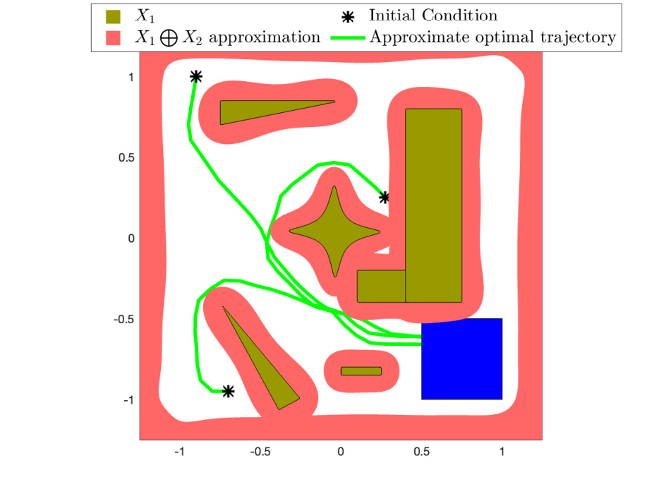
(a) Workspace
Refer to caption
(b) C-space
Figure 5: Plot associated with Example 5 showing collision free trajectories of Dubin’s car in both the workspace and C-space.

VII Conclusion

We have established a link between the L∞L^{\infty} and L1L^{1} function metrics and the Hausdorff and volume set metrics, respectively, allowing us to construct SOS programs for accurately approximating sets encountered throughout control theory. More specifically, we have shown that if functions are close in the L∞L^{\infty} norm and one uniformly bounds the other, their sublevel sets are close in the Hausdorff metric. Likewise, if we change the function metric to the L1L^{1} norm, the respective sublevel sets are close in the volume metric. By applying our methodology to approximating sets of discrete points, we have proposed a new machine learning one-class classification algorithm that accurately finds decision boundaries for problems with low-dimensional, error-free, and dense data sets. We have applied this new classification algorithm to the problem of approximating ROAs or attractor sets of nonlinear ODEs. Furthermore, our set approximation approach allows us to numerically approximate Minkowski sums, which can be used to compute optimal collision-free paths.

[Uncaptioned image] Morgan Jones received the MMath degree in mathematics from The University of Oxford, England in 2016 and PhD degree from Arizona State University, USA in 2021. Since 2022 he has been a lecturer in the department of Automatic Control and Systems Engineering at the University of Sheffield. His research primarily focuses on the estimation of reachable sets, attractors and regions of attraction for nonlinear ODEs. Furthermore, he has an interest in extensions of the dynamic programing framework to non-separable cost functions.

References

  • [1] Y. Guan and J. Wang, “Uncertainty sets for robust unit commitment,” IEEE Transactions on Power Systems, vol. 29, no. 3, pp. 1439–1440, 2013.
  • [2] M. Zhang, J. Fang, X. Ai, B. Zhou, W. Yao, Q. Wu, and J. Wen, “Partition-combine uncertainty set for robust unit commitment,” IEEE Transactions on Power Systems, vol. 35, no. 4, pp. 3266–3269, 2020.
  • [3] M. Jones and M. M. Peet, “Converse Lyapunov functions and converging inner approximations to maximal regions of attraction of nonlinear systems,” in 2021 60th IEEE Conference on Decision and Control (CDC), pp. 5312–5319, IEEE, 2021.
  • [4] D. Henrion and M. Korda, “Convex computation of the region of attraction of polynomial control systems,” IEEE Transactions on Automatic Control, vol. 59, no. 2, pp. 297–312, 2013.
  • [5] P. Trodden, “A one-step approach to computing a polytopic robust positively invariant set,” IEEE Transactions on Automatic Control, vol. 61, no. 12, pp. 4100–4105, 2016.
  • [6] M. Jones and M. M. Peet, “Polynomial approximation of value functions and nonlinear controller design with performance bounds,” arXiv preprint arXiv:2010.06828, 2020.
  • [7] M. Korda, D. Henrion, and C. N. Jones, “Convex computation of the maximum controlled invariant set for polynomial control systems,” SIAM Journal on Control and Optimization, vol. 52, no. 5, pp. 2944–2969, 2014.
  • [8] C. Schlosser, “Converging approximations of attractors via almost Lyapunov functions and semidefinite programming,” IEEE Control Systems Letters, vol. 6, pp. 2912–2917, 2022.
  • [9] M. Jones and M. M. Peet, “A converse Sum of Squares Lyapunov function for outer approximation of minimal attractor sets of nonlinear systems,” Journal of Computational Dynamics, vol. 10, no. 1, pp. 48–74, 2023.
  • [10] P. A. Trodden, J. M. Maestre, and H. Ishii, “Actuation attacks on constrained linear systems: A set-theoretic analysis,” IFAC-PapersOnLine, vol. 53, no. 2, pp. 6963–6968, 2020.
  • [11] F. Scibilia, S. Olaru, and M. Hovd, “On feasible sets for MPC and their approximations,” Automatica, vol. 47, no. 1, pp. 133–139, 2011.
  • [12] A. Magnani, S. Lall, and S. Boyd, “Tractable fitting with convex polynomials via Sum-of-Squares,” in Proceedings of the 44th IEEE Conference on Decision and Control, pp. 1672–1677, IEEE, 2005.
  • [13] A. A. Ahmadi, G. Hall, A. Makadia, and V. Sindhwani, “Geometry of 3D environments and Sum of Squares polynomials,” arXiv preprint arXiv:1611.07369, 2016.
  • [14] M. Jones and M. M. Peet, “Using SOS for optimal semialgebraic representation of sets: Finding minimal representations of limit cycles, chaotic attractors and unions,” in 2019 American Control Conference (ACC), pp. 2084–2091, IEEE, 2019.
  • [15] F. Dabbene and D. Henrion, “Set approximation via minimum-volume polynomial sublevel sets,” in 2013 European Control Conference (ECC), pp. 1114–1119, IEEE, 2013.
  • [16] D. Henrion, J. B. Lasserre, and C. Savorgnan, “Approximate volume and integration for basic semialgebraic sets,” SIAM review, vol. 51, no. 4, pp. 722–743, 2009.
  • [17] J. Guthrie, “Inner and outer approximations of star-convex semialgebraic sets,” IEEE Control Systems Letters, vol. 7, pp. 61–66, 2022.
  • [18] A. Cotorruelo, I. Kolmanovsky, and E. Garone, “A Sum-of-Squares-based procedure to approximate the Pontryagin difference of basic semi-algebraic sets,” Automatica, vol. 135, p. 109783, 2022.
  • [19] F. Dabbene, D. Henrion, and C. M. Lagoa, “Simple approximations of semialgebraic sets and their applications to control,” Automatica, vol. 78, pp. 110–118, 2017.
  • [20] J. B. Lasserre, “Tractable approximations of sets defined with quantifiers,” Mathematical Programming, vol. 151, pp. 507–527, 2015.
  • [21] H. T. Jongen and O. Stein, “Smoothing by mollifiers. part i: semi-infinite optimization,” Journal of Global Optimization, vol. 41, pp. 319–334, 2008.
  • [22] R. Kamyar and M. Peet, “Polynomial optimization with applications to stability analysis and control-alternatives to Sum of Squares,” Discrete and Continuous Dynamical Systems-Series B, vol. 20, no. 8, pp. 2383–2417, 2015.
  • [23] T. H. Pham, D. Ichalal, and S. Mammar, “Complete coverage path planning for pests-ridden in precision agriculture using UAV,” in 2020 IEEE International Conference on Networking, Sensing and Control (ICNSC), pp. 1–6, IEEE, 2020.
  • [24] J. Michaux, P. Holmes, B. Zhang, C. Chen, B. Wang, S. Sahgal, T. Zhang, S. Dey, S. Kousik, and R. Vasudevan, “Can’t touch this: Real-time, safe motion planning and control for manipulators under uncertainty,” arXiv preprint arXiv:2301.13308, 2023.
  • [25] S. Ruan and G. S. Chirikjian, “Closed-form Minkowski sums of convex bodies with smooth positively curved boundaries,” Computer-Aided Design, vol. 143, p. 103133, 2022.
  • [26] S. Ruan, K. L. Poblete, H. Wu, Q. Ma, and G. S. Chirikjian, “Efficient path planning in narrow passages for robots with ellipsoidal components,” IEEE Transactions on Robotics, 2022.
  • [27] J. Guthrie, M. Kobilarov, and E. Mallada, “Closed-form Minkowski sum approximations for efficient optimization-based collision avoidance,” in 2022 American Control Conference (ACC), pp. 3857–3864, IEEE, 2022.
  • [28] J. Lofberg, “YALMIP: A toolbox for modeling and optimization in MATLAB,” in 2004 IEEE international conference on robotics and automation (IEEE Cat. No. 04CH37508), pp. 284–289, IEEE, 2004.
  • [29] Mosek, “Mosek optimization toolbox for MATLAB,” User’s Guide and Reference Manual, Version, vol. 4, p. 1, 2019.
  • [30] L. L. Fernandes, M. Jones, L. Alberto, M. Peet, and D. Dotta, “Combining trajectory data with analytical Lyapunov functions for improved region of attraction estimation,” IEEE Control Systems Letters, vol. 7, pp. 271–276, 2022.
  • [31] J. Shena, K. Kaloudis, C. Merkatas, and M. A. Sanjuán, “On the approximation of basins of attraction using deep neural networks,” arXiv preprint arXiv:2109.06564, 2021.
  • [32] M. Jones and M. M. Peet, “A generalization of Bellman’s equation with application to path planning, obstacle avoidance and invariant set estimation,” Automatica, vol. 127, p. 109510, 2021.
  • [33] A. O’Farrell, “Five generalisations of the Weierstrass Approximation Theorem,” in Proceedings of the Royal Irish Academy. Section A: Mathematical and Physical Sciences, pp. 65–69, JSTOR, 1981.
  • [34] L. C. Evans et al., “Partial differential equations: graduate studies in mathematics,” 1998.
  • [35] G. Oman, “A short proof of the Bolzano-Weierstrass Theorem,” The College Mathematics Journal, 2017.
  • [36] M. Putinar, “Positive polynomials on compact semi-algebraic sets,” Indiana University Mathematics Journal, vol. 42, no. 3, pp. 969–984, 1993.
  • [37] F. H. Clarke, “Generalized gradients and applications,” Transactions of the American Mathematical Society, vol. 205, pp. 247–262, 1975.
  • [38] C. Schlosser and M. Korda, “Converging outer approximations to global attractors using semidefinite programming,” Automatica, vol. 134, p. 109900, 2021.

VIII Appendix

VIII-A The Volume Metric

Recall from Section III-B that

DV​(A,B):=μ⁡((A/B)∪(B/A)),\displaystyle D_{V}(A,B):=\mu((A/B)\cup(B/A)),

where μ⁡(A)\mu(A) is the Lebesgue measure of A⊂ℝnA\subset\mathbb{R}^{n}.

Definition 3.

D:X×X→ℝD:X\times X\to\mathbb{R} is a metric if the following is satisfied for all x,y∈Xx,y\in X,

  • •

    D⁡(x,y)≥0D(x,y)\geq 0,

  • •

    D⁡(x,y)=0D(x,y)=0 iff x=yx=y,

  • •

    D⁡(x,y)=D⁡(y,x)D(x,y)=D(y,x),

  • •

    D⁡(x,z)≤D⁡(x,y)+D⁡(y,z)D(x,z)\leq D(x,y)+D(y,z).

The sublevel approximation results presented in this appendix are required in the proof of Theorem 2.

Lemma 6 ([14]).

Consider the quotient space,

X:=ℬ(mod{X⊂ℝn:X≠∅,μ(X)=0}),X:=\mathcal{B}\pmod{\{X\subset\mathbb{R}^{n}:X\neq\emptyset,\mu(X)=0\}},

where ℬ\mathcal{B} is the set of all Lebesgue measurable sets. Then DV:X×X→ℝD_{V}:X\times X\to\mathbb{R} is a metric.

Lemma 7 ([14]).

Consider Lebesgue measurable sets A,B⊂ℝnA,B\subset\mathbb{R}^{n}. Suppose AA and BB have finite Lebesgue measure and B⊆AB\subseteq A, then

DV​(A,B)\displaystyle D_{V}(A,B) =μ⁡(A/B)=μ⁡(A)−μ⁡(B).\displaystyle=\mu(A/B)=\mu(A)-\mu(B).
Proposition 1 ([6]).

Consider a Lebesgue measurable set Λ⊂ℝn\Lambda\subset\mathbb{R}^{n} with finite Lebesgue measure, a function V∈L1​(Λ,ℝ)V\in L^{1}(\Lambda,\mathbb{R}), and a family of functions {Jd∈L1​(Λ,ℝ):d∈ℕ}\{J_{d}\in L^{1}(\Lambda,\mathbb{R}):d\in\mathbb{N}\} that satisfies the following properties:

  1. 1.

    For any d∈ℕd\in\mathbb{N} we have Jd​(x)≤V​(x)J_{d}(x)\leq V(x) for all x∈Λx\in\Lambda.

  2. 2.

    limd→∞‖V−Jd‖L1​(Λ,ℝ)=0\lim_{d\to\infty}||V-J_{d}||_{L^{1}(\Lambda,\mathbb{R})}=0.

Then for all γ∈ℝ\gamma\in\mathbb{R}

limd→∞DV​({x∈Λ:V⁡(x)≤γ},{x∈Λ:Jd​(x)≤γ})=0.\displaystyle\lim_{d\to\infty}D_{V}\bigg(\{x\in\Lambda:V(x)\leq\gamma\},\{x\in\Lambda:J_{d}(x)\leq\gamma\}\bigg)=0. (67)

VIII-B Counterexamples: When Close Functions Have Distant Sublevel Sets

As pointed out by Remark 1, relaxing the statement of Thm. 1 in any way may result in the loss of sublevel set convergence. We first show that if we slightly change the conditions of Thm. 1 to have Jd​(x)≤V​(x)J_{d}(x)\leq V(x) (rather than V​(x)≤Jd​(x)V(x)\leq J_{d}(x)) then we can no longer establish that the sublevel sets of VV and JdJ_{d} will be close.

Counterexample 1 (Upper functional approximation is important).

We show there exists γ∈ℝ\gamma\in\mathbb{R}, Λ⊂ℝ\Lambda\subset\mathbb{R}, V∈L1​(Λ,ℝ)V\in L^{1}(\Lambda,\mathbb{R}) and {Jd}d∈ℕ⊂L1​(Λ,ℝ)\{J_{d}\}_{d\in\mathbb{N}}\subset L^{1}(\Lambda,\mathbb{R}) such that Jd​(x)≤V​(x)J_{d}(x)\leq V(x) for all x∈Λx\in\Lambda and limd→∞‖V⁡(x)−Jd​(x)‖L∞​(Λ,ℝ)​d​x=0\lim_{d\to\infty}||V(x)-J_{d}(x)||_{L^{\infty}(\Lambda,\mathbb{R})}dx=0 but

limd→∞DH​({x∈Λ:V⁡(x)<γ},{x∈Λ:Jd​(x)<γ})≠0.\displaystyle\lim_{d\to\infty}D_{H}\bigg(\{x\in\Lambda:V(x)<\gamma\},\{x\in\Lambda:J_{d}(x)<\gamma\}\bigg)\neq 0.

Let Λ:=[−10,10]\Lambda:=[-10,10], γ:=1\gamma:=1, V⁡(x):=1−𝟙[1,2]​(x)V(x):=1-\mathds{1}_{[1,2]}(x) and Jd​(x)=1−𝟙[1,2]​(x)−1dJ_{d}(x)=1-\mathds{1}_{[1,2]}(x)-\frac{1}{d}. The functions, along with their corresponding sublevel sets highlighted, have been graphically represented in Fig. 6. Clearly, limd→∞‖V⁡(x)−Jd​(x)‖L∞​(Λ,ℝ)​d​x=limd→∞1d=0\lim_{d\to\infty}||V(x)-J_{d}(x)||_{L^{\infty}(\Lambda,\mathbb{R})}dx=\lim_{d\to\infty}\frac{1}{d}=0. However,

{x∈Λ:V⁡(x)<1}\displaystyle\{x\in\Lambda:V(x)<1\} =[1,2].\displaystyle=[1,2].
{x∈Λ:Jd​(x)<1}\displaystyle\{x\in\Lambda:J_{d}(x)<1\} =Λ.\displaystyle=\Lambda.

Note, Counterexample 1 does not contradict Prop. 1 that deals with the same case where JdJ_{d} lower bounds VV. This is because Prop. 1 shows that the non-strict sublevel sets are close in the volume metric. Indeed, {x∈Λ:V⁡(x)≤1}={x∈Λ:Jd​(x)≤1}\{x\in\Lambda:V(x)\leq 1\}=\{x\in\Lambda:J_{d}(x)\leq 1\} so there is no contradiction in this case.

We next consider what happens if we change the other condition of Thm. 1 where instead of having ‖Jd−V‖L∞​(Λ,ℝ)→0||J_{d}-V||_{L^{\infty}(\Lambda,\mathbb{R})}\to 0 we only have ‖Jd−V‖L1​(Λ,ℝ)→0||J_{d}-V||_{L^{1}(\Lambda,\mathbb{R})}\to 0.

Counterexample 2 (L∞L^{\infty} functional approximation is important).

We show there exists γ∈ℝ\gamma\in\mathbb{R}, Λ⊂ℝ\Lambda\subset\mathbb{R}, V∈L1​(Λ,ℝ)V\in L^{1}(\Lambda,\mathbb{R}) and {Jd}d∈ℕ⊂L1​(Λ,ℝ)\{J_{d}\}_{d\in\mathbb{N}}\subset L^{1}(\Lambda,\mathbb{R}) such that V​(x)≤Jd​(x)V(x)\leq J_{d}(x) for all x∈Λx\in\Lambda and limd→∞‖V⁡(x)−Jd​(x)‖L1​(Λ,ℝ)=0\lim_{d\to\infty}||V(x)-J_{d}(x)||_{L^{1}(\Lambda,\mathbb{R})}=0 but

limd→∞DH​({x∈Λ:V⁡(x)<γ},{x∈Λ:Jd​(x)<γ})≠0.\displaystyle\lim_{d\to\infty}D_{H}\bigg(\{x\in\Lambda:V(x)<\gamma\},\{x\in\Lambda:J_{d}(x)<\gamma\}\bigg)\neq 0.

Let Λ:=[−10,10]\Lambda:=[-10,10], γ:=1\gamma:=1, V⁡(x):=1−𝟙{0.5}​(x)−𝟙[1,2]​(x)V(x):=1-\mathds{1}_{\{0.5\}}(x)-\mathds{1}_{[1,2]}(x) and Jd​(x):=1−𝟙[1,2−1/d]​(x)J_{d}(x):=1-\mathds{1}_{[1,2-\nicefrac{{1}}{{d}}]}(x). The functions, along with their corresponding sublevel sets highlighted, have been graphically represented in Fig. 7. Clearly, limd→∞‖V⁡(x)−Jd​(x)‖L∞​(Λ,ℝ)=limd→∞supx∈Λ{𝟙{0.5}​(x)+𝟙[2−1/d,2]​(x)}=1≠0\lim_{d\to\infty}||V(x)-J_{d}(x)||_{L^{\infty}(\Lambda,\mathbb{R})}=\lim_{d\to\infty}\sup_{x\in\Lambda}\{\mathds{1}_{\{0.5\}}(x)+\mathds{1}_{[2-\nicefrac{{1}}{{d}},2]}(x)\}=1\neq 0 and limd→∞‖V⁡(x)−Jd​(x)‖L1​(Λ,ℝ)=limd→∞∫Λ𝟙{0.5}​(x)+𝟙[2−1/d,2]​(x)​𝑑x=limd→∞∫2−1/d21​𝑑x=limd→∞1d=0\lim_{d\to\infty}||V(x)-J_{d}(x)||_{L^{1}(\Lambda,\mathbb{R})}=\lim_{d\to\infty}\int_{\Lambda}\mathds{1}_{\{0.5\}}(x)+\mathds{1}_{[2-\nicefrac{{1}}{{d}},2]}(x)dx=\lim_{d\to\infty}\int_{2-\nicefrac{{1}}{{d}}}^{2}1dx=\lim_{d\to\infty}\frac{1}{d}=0. However,

{x∈Λ:V⁡(x)<1}\displaystyle\{x\in\Lambda:V(x)<1\} =[1,2]∪{0.5}.\displaystyle=[1,2]\cup\{0.5\}.
{x∈Λ:Jd​(x)<1}\displaystyle\{x\in\Lambda:J_{d}(x)<1\} =[1,2−1/d].\displaystyle=[1,2-\nicefrac{{1}}{{d}}].

Hence

limd→∞DH​({x∈Λ:V⁡(x)<γ},{x∈Λ:Jd​(x)<γ})\displaystyle\lim_{d\to\infty}D_{H}\bigg(\{x\in\Lambda:V(x)<\gamma\},\{x\in\Lambda:J_{d}(x)<\gamma\}\bigg)
=limd→∞DH​([1,2]∪{0.5},[1,2−1/d])=0.5≠0.\displaystyle=\lim_{d\to\infty}D_{H}([1,2]\cup\{0.5\},[1,2-\nicefrac{{1}}{{d}}])=0.5\neq 0.

Although Counterexample 2 shows that if functions are close in the L1L^{1} norm then their sublevel sets may not be close in the Hausdorff metric this does not contradict Theorem 2, that shows that these sublevel sets must be close in the volume metric. This holds true in the case of Counterexample 2 since

limd→∞DV​({x∈Λ:V⁡(x)<γ},{x∈Λ:Jd​(x)<γ})\displaystyle\lim_{d\to\infty}D_{V}\bigg(\{x\in\Lambda:V(x)<\gamma\},\{x\in\Lambda:J_{d}(x)<\gamma\}\bigg)
=limd→∞DV​([1,2]∪{0.5},[1,2−1/d])\displaystyle=\lim_{d\to\infty}D_{V}([1,2]\cup\{0.5\},[1,2-\nicefrac{{1}}{{d}}])
=limd→∞μ⁡([2−1/d,2]∪{0.5})=0.\displaystyle=\lim_{d\to\infty}\mu([2-\nicefrac{{1}}{{d}},2]\cup\{0.5\})=0.

Note that in the case of approximating discrete points we approximate V⁡(x)=1−𝟙{xi}i=1N​(x)V(x)=1-\mathds{1}_{\{x_{i}\}_{i=1}^{N}}(x) using Opt. (40). Since, in this case, VV is discontinuous we cannot approximate it in the L∞L^{\infty} norm by a smooth function (like a polynomial). Counterexample 2 shows that this L1L^{1} approximation may not be sufficient to approximate discrete points in the Hausdorff metric but Theorem 2 shows that we can still use Opt. (40) to approximate discrete points in the volume metric.

xxyy111122V⁡(x)=1−𝟙[1,2]​(x)V(x)=1-\mathds{1}_{[1,2]}(x)Jd​(x)=1−𝟙[1,2]​(x)−1/dJ_{d}(x)=1-\mathds{1}_{[1,2]}(x)-\nicefrac{{1}}{{d}}={x∈Λ:V⁡(x)<1}=\{x\in\Lambda:V(x)<1\}={x∈Λ:Jd​(x)<1}=\{x\in\Lambda:J_{d}(x)<1\}
Figure 6: Figure associated with Counterexample 1 showing {x∈Λ:Jd​(x)<1}↛{x∈Λ:V⁡(x)<1}\{x\in\Lambda:J_{d}(x)<1\}\not\to\{x\in\Lambda:V(x)<1\} even when Jd→VJ_{d}\to V in the L∞L^{\infty} norm from below.
xxyy1111220.50.5V⁡(x)=1−𝟙{0.5}​(x)−𝟙[1,2]​(x)V(x)=1-\mathds{1}_{\{0.5\}}(x)-\mathds{1}_{[1,2]}(x)Jd​(x)=1−𝟙[1,2−1/d]​(x)J_{d}(x)=1-\mathds{1}_{[1,2-\nicefrac{{1}}{{d}}]}(x)={x∈Λ:V⁡(x)<1}=\{x\in\Lambda:V(x)<1\}={x∈Λ:Jd​(x)<1}=\{x\in\Lambda:J_{d}(x)<1\}
Figure 7: Figure associated with Counterexample 2 showing {x∈Λ:Jd​(x)<1}↛{x∈Λ:V⁡(x)<1}\{x\in\Lambda:J_{d}(x)<1\}\not\to\{x\in\Lambda:V(x)<1\} in the Hausdorff metric even when Jd→VJ_{d}\to V in the L1L^{1} norm from above.

We next consider what happens if we modify the statements of Theorems 1 and 2 that the non-strict sublevel sets converge, rather than the strict sublevel sets converge.

Counterexample 3 (Strictness of the sublevel set is important).

We show there exists γ∈ℝ\gamma\in\mathbb{R}, Λ⊂ℝ\Lambda\subset\mathbb{R}, V∈L1​(Λ,ℝ)V\in L^{1}(\Lambda,\mathbb{R}) and {Jd}d∈ℕ⊂L1​(Λ,ℝ)\{J_{d}\}_{d\in\mathbb{N}}\subset L^{1}(\Lambda,\mathbb{R}) such that V​(x)≤Jd​(x)V(x)\leq J_{d}(x) for all x∈Λx\in\Lambda and limd→∞‖V⁡(x)−Jd​(x)‖L∞​(Λ,ℝ)=0\lim_{d\to\infty}||V(x)-J_{d}(x)||_{L^{\infty}(\Lambda,\mathbb{R})}=0 but

limd→∞DH​({x∈Λ:V⁡(x)≤γ},{x∈Λ:Jd​(x)≤γ})≠0,\displaystyle\lim_{d\to\infty}D_{H}\bigg(\{x\in\Lambda:V(x)\leq\gamma\},\{x\in\Lambda:J_{d}(x)\leq\gamma\}\bigg)\neq 0,
limd→∞DV​({x∈Λ:V⁡(x)≤γ},{x∈Λ:Jd​(x)≤γ})≠0.\displaystyle\lim_{d\to\infty}D_{V}\bigg(\{x\in\Lambda:V(x)\leq\gamma\},\{x\in\Lambda:J_{d}(x)\leq\gamma\}\bigg)\neq 0.

Let Λ:=[0,3]\Lambda:=[0,3], γ:=1\gamma:=1, V⁡(x):=1−𝟙[1,2]​(x)V(x):=1-\mathds{1}_{[1,2]}(x) and Jd​(x):=1−𝟙[1,2]​(x)+1/d​𝟙[2,2.5]​(x)J_{d}(x):=1-\mathds{1}_{[1,2]}(x)+\nicefrac{{1}}{{d}}\mathds{1}_{[2,2.5]}(x). The functions, along with their corresponding sublevel sets highlighted, have been graphically represented in Fig. 8. Clearly, limd→∞||V(x)−Jd(x)||L∞​(Λ,ℝ)=limd→∞supx∈Λ{1/d𝟙[2,2.5](x))}=limd→∞1/d=0\lim_{d\to\infty}||V(x)-J_{d}(x)||_{L^{\infty}(\Lambda,\mathbb{R})}=\lim_{d\to\infty}\sup_{x\in\Lambda}\{\nicefrac{{1}}{{d}}\mathds{1}_{[2,2.5]}(x))\}=\lim_{d\to\infty}\nicefrac{{1}}{{d}}=0. However,

{x∈Λ:V⁡(x)≤1}\displaystyle\{x\in\Lambda:V(x)\leq 1\} =Λ=[0,3].\displaystyle=\Lambda=[0,3].
{x∈Λ:Jd​(x)≤1}\displaystyle\{x\in\Lambda:J_{d}(x)\leq 1\} =[0,2)∪(2.5,3].\displaystyle=[0,2)\cup(2.5,3].

Hence,

limd→∞DH​({x∈Λ:V⁡(x)≤γ},{x∈Λ:Jd​(x)≤γ})\displaystyle\lim_{d\to\infty}D_{H}\bigg(\{x\in\Lambda:V(x)\leq\gamma\},\{x\in\Lambda:J_{d}(x)\leq\gamma\}\bigg)
=limd→∞DH​([0,3],[0,2)∪(2.5,3])=0.25≠0,\displaystyle=\lim_{d\to\infty}D_{H}([0,3],[0,2)\cup(2.5,3])=0.25\neq 0,

Moroever,

limd→∞DV​({x∈Λ:V⁡(x)≤γ},{x∈Λ:Jd​(x)≤γ})\displaystyle\lim_{d\to\infty}D_{V}\bigg(\{x\in\Lambda:V(x)\leq\gamma\},\{x\in\Lambda:J_{d}(x)\leq\gamma\}\bigg)
=limd→∞DV​([0,3],[0,2)∪(2.5,3])=μ⁡([2,2.5])=0.5≠0.\displaystyle=\lim_{d\to\infty}D_{V}([0,3],[0,2)\cup(2.5,3])=\mu([2,2.5])=0.5\neq 0.
xxyy111122V⁡(x)=1−𝟙[1,2]​(x)V(x)=1-\mathds{1}_{[1,2]}(x)Jd​(x)=1−𝟙[1,2]​(x)+1/d​𝟙[2,2.5]​(x)J_{d}(x)=1-\mathds{1}_{[1,2]}(x)+\nicefrac{{1}}{{d}}\mathds{1}_{[2,2.5]}(x)={x∈Λ:V⁡(x)≤1}=\{x\in\Lambda:V(x)\leq 1\}={x∈Λ:Jd​(x)≤1}=\{x\in\Lambda:J_{d}(x)\leq 1\}
Figure 8: Figure associated with Counterexample 3 showing {x∈Λ:Jd​(x)≤1}↛{x∈Λ:V⁡(x)≤1}\{x\in\Lambda:J_{d}(x)\leq 1\}\not\to\{x\in\Lambda:V(x)\leq 1\} in the Hausdorff and volume metric even when Jd→VJ_{d}\to V in the L∞L^{\infty} norm from above.
={x∈Λ:V⁡(x)<1}=\{x\in\Lambda:V(x)<1\}={x∈Λ:Jd​(x)<1}=\{x\in\Lambda:J_{d}(x)<1\}V⁡(x)=1−𝟙[1,2]​(x)V(x)=1-\mathds{1}_{[1,2]}(x)Jd​(x)=1−𝟙[1,2]​(x)+1/d​𝟙[2,2.5]​(x)J_{d}(x)=1-\mathds{1}_{[1,2]}(x)+\nicefrac{{1}}{{d}}\mathds{1}_{[2,2.5]}(x)V⁡(x)=−e−xV(x)=-e^{-x}Jd​(x)=1/d−e−xJ_{d}(x)=\nicefrac{{1}}{{d}}-e^{-x}ln⁡(d)\ln(d)
Figure 9: Figure associated with Counterexample 4 showing {x∈Λ:Jd​(x)<1}↛{x∈Λ:V⁡(x)<1}\{x\in\Lambda:J_{d}(x)<1\}\not\to\{x\in\Lambda:V(x)<1\} in the Hausdorff or volume metric even when Jd→VJ_{d}\to V in the L∞L^{\infty} norm from above if Λ\Lambda is not compact.

We next show that if we relax the condition that Λ⊂ℝn\Lambda\subset\mathbb{R}^{n} is compact in Theorem 1, or the condition Λ⊂ℝn\Lambda\subset\mathbb{R}^{n} has finite Lebesque measure Theorem 2, then we may not get sublevel set convergence.

Counterexample 4 (Compactness of sublevel set domain is important).

We show there exists γ∈ℝ\gamma\in\mathbb{R}, non-compact Λ⊂ℝ\Lambda\subset\mathbb{R}, V∈L1​(Λ,ℝ)V\in L^{1}(\Lambda,\mathbb{R}) and {Jd}d∈ℕ⊂L1​(Λ,ℝ)\{J_{d}\}_{d\in\mathbb{N}}\subset L^{1}(\Lambda,\mathbb{R}) such that V​(x)≤Jd​(x)V(x)\leq J_{d}(x) for all x∈Λx\in\Lambda and limd→∞‖V⁡(x)−Jd​(x)‖L∞​(Λ,ℝ)=0\lim_{d\to\infty}||V(x)-J_{d}(x)||_{L^{\infty}(\Lambda,\mathbb{R})}=0 but

limd→∞DH​({x∈Λ:V⁡(x)<γ},{x∈Λ:Jd​(x)<γ})≠0.\displaystyle\lim_{d\to\infty}D_{H}\bigg(\{x\in\Lambda:V(x)<\gamma\},\{x\in\Lambda:J_{d}(x)<\gamma\}\bigg)\neq 0.

Let Λ=[0,∞)\Lambda=[0,\infty), γ=0\gamma=0, V⁡(x)=−e−xV(x)=-e^{-x} and Jd​(x)=1/d−e−xJ_{d}(x)=\nicefrac{{1}}{{d}}-e^{-x}. The functions, along with their corresponding sublevel sets highlighted, have been graphically represented in Fig. 9. Clearly, limd→∞‖V⁡(x)−Jd​(x)‖L∞​(Λ,ℝ)=limd→∞1/d=0\lim_{d\to\infty}||V(x)-J_{d}(x)||_{L^{\infty}(\Lambda,\mathbb{R})}=\lim_{d\to\infty}\nicefrac{{1}}{{d}}=0. However,

{x∈Λ:V⁡(x)<0}\displaystyle\{x\in\Lambda:V(x)<0\} =Λ=[0,∞).\displaystyle=\Lambda=[0,\infty).
{x∈Λ:Jd​(x)<0}\displaystyle\{x\in\Lambda:J_{d}(x)<0\} =[0,ln⁡(d)).\displaystyle=[0,\ln(d)).

Hence,

limd→∞DH​({x∈Λ:V⁡(x)<γ},{x∈Λ:Jd​(x)<γ})\displaystyle\lim_{d\to\infty}D_{H}\bigg(\{x\in\Lambda:V(x)<\gamma\},\{x\in\Lambda:J_{d}(x)<\gamma\}\bigg)
=limd→∞DH​([0,∞),[0,ln⁡(d)))=∞≠0,\displaystyle=\lim_{d\to\infty}D_{H}([0,\infty),[0,\ln(d)))=\infty\neq 0,

VIII-C Polynomial Approximation

In Sec. IV we characterized several sets (intersections and unions of semialgebraic sets, Minkowski sums, Pontryagin differences and discrete points) by sublevel sets of various functions. We now show that we can approximate these functions arbitrarily well by polynomials that are also feasible to our associated SOS optimization problems. In order to approximate these functions we use the Weierstrass approximation theorem.

Theorem 6 (Weierstrass approximation theorem [33]).

Let E⊂ℝnE\subset\mathbb{R}^{n} be an open set and f∈C1​(E,ℝ)f\in C^{1}(E,\mathbb{R}). For any compact set K⊆EK\subseteq E and ε>0\varepsilon>0 there exists g∈ℝ⁡[x]g\in\mathbb{R}[x] such that

supx∈K|f⁡(x)−g⁡(x)|<ε.\displaystyle\sup_{x\in K}|f(x)-g(x)|<\varepsilon.

We next show that there exists a polynomial that is feasible to Opt. (26) and that arbitrarily approximates the function, V⁡(x):=min1≤i≤m⁡gi​(x)V(x):=\min_{1\leq i\leq m}g_{i}(x), whose sublevel set characterizes the set given in Eq. (25).

Proposition 2.

Consider a compact set Λ⊂ℝn\Lambda\subset\mathbb{R}^{n}, functions gi∈L​o​c​L​i​p​(Λ,ℝ)g_{i}\in LocLip(\Lambda,\mathbb{R}) for 1≤i≤m1\leq i\leq m, a scalar r>0r>0, and V⁡(x):=min1≤i≤m⁡{gi​(x)}V(x):=\min_{1\leq i\leq m}\{g_{i}(x)\}. Then for any ε>0\varepsilon>0 there exists H1,H2∈ℝ⁡[x]H_{1},H_{2}\in\mathbb{R}[x] such that

supx∈Λ|V⁡(x)−Hj​(x)|<ε​ for ​j∈{1,2},\displaystyle\sup_{x\in\Lambda}|V(x)-H_{j}(x)|<\varepsilon\text{ for }j\in\{1,2\}, (68)
H1​(x)<gi​(x)​ for all ​x∈Br​(0)​ and ​1≤i≤m,\displaystyle H_{1}(x)<g_{i}(x)\text{ for all }x\in B_{r}(0)\text{ and }1\leq i\leq m,
H2​(x)>gi​(x)​ for all ​x∈Br​(0)∩𝒴i¯​ and ​1≤i≤m,\displaystyle H_{2}(x)>g_{i}(x)\text{ for all }x\in B_{r}(0)\cap\underline{\mathcal{Y}_{i}}\text{ and }1\leq i\leq m,

where 𝒴i¯:={y∈Λ:gi​(y)≤gj​(y)​ for ​1≤j≤m}\underline{\mathcal{Y}_{i}}:=\{y\in\Lambda:g_{i}(y)\leq g_{j}(y)\text{ for }1\leq j\leq m\}.

Proof.

We first show the existence of H1∈ℝ⁡[x]H_{1}\in\mathbb{R}[x] that satisfies Eq. (68). Since Λ⊂ℝn\Lambda\subset\mathbb{R}^{n} and Br​(0)B_{r}(0) are compact sets it follows that there exists R>0R>0 such that Λ∪Br​(0)⊂BR​(0)\Lambda\cup B_{r}(0)\subset B_{R}(0). Let ε>0\varepsilon>0. Since VV is continuous by Lem. 9 it follows by Thm. 6 that there exists P∈ℝ⁡[x]P\in\mathbb{R}[x] such that supx∈BR​(0)|V⁡(x)−P⁡(x)|<ε/4\sup_{x\in B_{R}(0)}|V(x)-P(x)|<\varepsilon/4. Let H1​(x):=P⁡(x)−ε/4H_{1}(x):=P(x)-\varepsilon/4. Then

|V​(x)−H1​(x)|\displaystyle|V(x)-H_{1}(x)| =|V⁡(x)−P⁡(x)+ε/2|<|V⁡(x)−P⁡(x)|+ε/4\displaystyle=|V(x)-P(x)+\varepsilon/2|<|V(x)-P(x)|+\varepsilon/4
<ε/2​ for all ​x∈BR​(0),\displaystyle<\varepsilon/2\text{ for all }x\in B_{R}(0),

and hence supx∈Λ|V⁡(x)−H1​(x)|≤ε/2<ε\sup_{x\in\Lambda}|V(x)-H_{1}(x)|\leq\varepsilon/2<\varepsilon.

Moreover, since |V⁡(x)−P⁡(x)|<ε/4|V(x)-P(x)|<\varepsilon/4 for all x∈BR​(0)x\in B_{R}(0) we have that P⁡(x)<V⁡(x)+ε/4P(x)<V(x)+\varepsilon/4 for all x∈BR​(0)x\in B_{R}(0) . Hence H1​(x)<V⁡(x)+ε/4−ε/4=V⁡(x)=min1≤j≤m⁡{gj​(x)}≤gi​(x)H_{1}(x)<V(x)+\varepsilon/4-\varepsilon/4=V(x)=\min_{1\leq j\leq m}\{g_{j}(x)\}\leq g_{i}(x) for all 1≤i≤m1\leq i\leq m and x∈Br​(0)⊂BR​(0)x\in B_{r}(0)\subset B_{R}(0).

We next show the existence of H2∈ℝ⁡[x]H_{2}\in\mathbb{R}[x] that satisfies Eq. (68). This time let H2​(x):=P⁡(x)+ε/4H_{2}(x):=P(x)+\varepsilon/4. Then

|V​(x)−H2​(x)|\displaystyle|V(x)-H_{2}(x)| =|V⁡(x)−P⁡(x)−ε/2|<|V⁡(x)−P⁡(x)|+ε/4\displaystyle=|V(x)-P(x)-\varepsilon/2|<|V(x)-P(x)|+\varepsilon/4
<ε/2​ for all ​x∈BR​(0),\displaystyle<\varepsilon/2\text{ for all }x\in B_{R}(0),

and hence supx∈Λ|V⁡(x)−H2​(x)|<ε\sup_{x\in\Lambda}|V(x)-H_{2}(x)|<\varepsilon.

Moreover, since |V⁡(x)−P⁡(x)|<ε/4|V(x)-P(x)|<\varepsilon/4 for all x∈BR​(0)x\in B_{R}(0) we have that P⁡(x)>V⁡(x)−ε/4P(x)>V(x)-\varepsilon/4 for all x∈BR​(0)x\in B_{R}(0). Hence H2​(x)>V⁡(x)−ε/4+ε/4=V⁡(x)H_{2}(x)>V(x)-\varepsilon/4+\varepsilon/4=V(x) for all x∈BR​(0)x\in B_{R}(0). Now, when x∈𝒴i¯x\in\underline{\mathcal{Y}_{i}} we have V​(x)=gi​(x)V(x)=g_{i}(x). Therefore, H2​(x)>V⁡(x)=gi​(x)H_{2}(x)>V(x)=g_{i}(x) for all x∈𝒴i¯∩Br​(0)x\in\underline{\mathcal{Y}_{i}}\cap B_{r}(0).

∎

We next show that there exists a polynomial that is feasible to Opt. (23) and that arbitrarily approximates the function, V⁡(x):=max1≤i≤m⁡gi​(x)V(x):=\max_{1\leq i\leq m}g_{i}(x), whose sublevel set characterizes the set given in Eq. (22).

Corollary 1.

Consider a compact set Λ⊂ℝn\Lambda\subset\mathbb{R}^{n}, gi∈L​o​c​L​i​p​(Λ,ℝ)g_{i}\in LocLip(\Lambda,\mathbb{R}) for 1≤i≤m1\leq i\leq m and V⁡(x):=max1≤i≤m⁡{gi​(x)}V(x):=\max_{1\leq i\leq m}\{g_{i}(x)\}. Then for any ε>0\varepsilon>0 there exists H1,H2∈ℝ⁡[x]H_{1},H_{2}\in\mathbb{R}[x] such that

supx∈Λ|V⁡(x)−Hj​(x)|<ε​ for ​j∈{1,2},\displaystyle\sup_{x\in\Lambda}|V(x)-H_{j}(x)|<\varepsilon\text{ for }j\in\{1,2\}, (69)
H1​(x)>gi​(x)​ for all ​x∈Br​(0)​ and ​1≤i≤m,\displaystyle H_{1}(x)>g_{i}(x)\text{ for all }x\in B_{r}(0)\text{ and }1\leq i\leq m,
H2​(x)<gi​(x)​ for all ​x∈Br​(0)∩𝒴i¯​ and ​1≤i≤m,\displaystyle H_{2}(x)<g_{i}(x)\text{ for all }x\in B_{r}(0)\cap\bar{\mathcal{Y}_{i}}\text{ and }1\leq i\leq m,

where 𝒴i¯:={y∈Λ:gi​(y)≥gj​(y)​ for ​1≤j≤m}\bar{\mathcal{Y}_{i}}:=\{y\in\Lambda:g_{i}(y)\geq g_{j}(y)\text{ for }1\leq j\leq m\}.

Proof.

Note that max1≤i≤m⁡{gi​(x)}=−min1≤i≤m⁡{−gi​(x)}\max_{1\leq i\leq m}\{g_{i}(x)\}=-\min_{1\leq i\leq m}\{-g_{i}(x)\}. Let V~​(x):=min1≤i≤m⁡{−gi​(x)}=−V⁡(x)\tilde{V}(x):=\min_{1\leq i\leq m}\{-g_{i}(x)\}=-V(x). By Prop. 2 there exists H1~,H2~∈ℝ⁡[x]\tilde{H_{1}},\tilde{H_{2}}\in\mathbb{R}[x] such that

supx∈Λ|V~​(x)−Hj~​(x)|<ε​ for ​j∈{1,2},\displaystyle\sup_{x\in\Lambda}|\tilde{V}(x)-\tilde{H_{j}}(x)|<\varepsilon\text{ for }j\in\{1,2\},
H1~​(x)<−gi​(x)​ for all ​x∈Br​(0)​ and ​1≤i≤m,\displaystyle\tilde{H_{1}}(x)<-g_{i}(x)\text{ for all }x\in B_{r}(0)\text{ and }1\leq i\leq m,
H2~​(x)>−gi​(x)​ for all ​x∈Br​(0)∩𝒴i¯~​ and ​1≤i≤m,\displaystyle\tilde{H_{2}}(x)>-g_{i}(x)\text{ for all }x\in B_{r}(0)\cap\tilde{\underline{\mathcal{Y}_{i}}}\text{ and }1\leq i\leq m,

where 𝒴i¯~:={y∈Λ:−gi​(y)≤−gj​(y)​ for ​1≤j≤m}={y∈Λ:gi​(y)≥gj​(y)​ for ​1≤j≤m}=𝒴i¯\tilde{\underline{\mathcal{Y}_{i}}}:=\{y\in\Lambda:-g_{i}(y)\leq-g_{j}(y)\text{ for }1\leq j\leq m\}=\{y\in\Lambda:g_{i}(y)\geq g_{j}(y)\text{ for }1\leq j\leq m\}=\bar{\mathcal{Y}_{i}}.

Let H1​(x):=−H1~​(x)H_{1}(x):=-\tilde{H_{1}}(x) and H2​(x):=−H2~​(x)H_{2}(x):=-\tilde{H_{2}}(x). Clearly H1H_{1} and H2H_{2} satisfies Eq. (69), completing the proof. ∎

We next show that there exists a polynomial that is feasible to Opt. (33) and that arbitrarily approximates the function, V(x):=infw∈{z∈Λ:g2,i​(z)≤0​ for ​1≤i≤m2}min1≤i≤m1g1,i(x−w)V(x):=\inf_{w\in\{z\in\Lambda:g_{2,i}(z)\leq 0\text{ for }1\leq i\leq m_{2}\}}\min_{1\leq i\leq m_{1}}g_{1,i}(x-w), whose sublevel set characterizes the set given in Eq. (31).

Lemma 8.

Consider a compact set Λ⊂ℝn\Lambda\subset\mathbb{R}^{n}, gi∈L​o​c​L​i​p​(Λ,ℝ)g_{i}\in LocLip(\Lambda,\mathbb{R}) for 1≤i≤m1\leq i\leq m and V(x):=infw∈{z∈Λ:g2,i​(z)≤0​ for ​1≤i≤m2}min1≤i≤m1g1,i(x−w)V(x):=\inf_{w\in\{z\in\Lambda:g_{2,i}(z)\leq 0\text{ for }1\leq i\leq m_{2}\}}\min_{1\leq i\leq m_{1}}g_{1,i}(x-w). Then for any ε>0\varepsilon>0 there exists H∈ℝ⁡[x]H\in\mathbb{R}[x] such that

supx∈Λ|V⁡(x)−H⁡(x)|<ε,\displaystyle\sup_{x\in\Lambda}|V(x)-H(x)|<\varepsilon, (70)
H⁡(x)<g1,i​(x−w)​ for all ​x∈Br​(0),\displaystyle H(x)<g_{1,i}(x-w)\text{ for all }x\in B_{r}(0),
w∈{z∈Λ:g2,j​(z)≤0​ for ​1≤j≤m2}​ and ​1≤i≤m1.\displaystyle\qquad w\in\{z\in\Lambda:g_{2,j}(z)\leq 0\text{ for }1\leq j\leq m_{2}\}\text{ and }1\leq i\leq m_{1}.
Proof.

Since Λ⊂ℝn\Lambda\subset\mathbb{R}^{n} and Br​(0)B_{r}(0) are compact sets there exists R>0R>0 such that Λ∪Br​(0)⊂BR​(0)\Lambda\cup B_{r}(0)\subset B_{R}(0). Now, by Lem. 9 it follows that VV is a continuous function. Hence, by Thm. 6, for any ε>0\varepsilon>0 there exists a polynomial P∈ℝ⁡[x]P\in\mathbb{R}[x] such that

supx∈BR​(0)|V⁡(x)−P⁡(x)|<ε4.\displaystyle\sup_{x\in B_{R}(0)}|V(x)-P(x)|<\frac{\varepsilon}{4}.

Let us consider H⁡(x):=P⁡(x)−ε4H(x):=P(x)-\frac{\varepsilon}{4}. Then

|V⁡(x)−H⁡(x)|≤|V⁡(x)−P⁡(x)|+ε4<ε2​ for ​x∈BR​(0).\displaystyle|V(x)-H(x)|\leq|V(x)-P(x)|+\frac{\varepsilon}{4}<\frac{\varepsilon}{2}\text{ for }x\in B_{R}(0).

Hence, supx∈Λ|V⁡(x)−H⁡(x)|<ε\sup_{x\in\Lambda}|V(x)-H(x)|<\varepsilon.

Also note that since |V⁡(x)−P⁡(x)|<ε4|V(x)-P(x)|<\frac{\varepsilon}{4} for all x∈BR​(0)x\in B_{R}(0) it follows that P⁡(x)<V⁡(x)+ε4P(x)<V(x)+\frac{\varepsilon}{4} and hence H⁡(x)=P⁡(x)−ε4<V⁡(x)H(x)=P(x)-\frac{\varepsilon}{4}<V(x) for all x∈Br​(0)⊂BR​(0)x\in B_{r}(0)\subset B_{R}(0). Therefore

P⁡(x)\displaystyle P(x) <V(x)=infu∈{z∈Λ:g2,j​(z)≤0​ for ​1≤j≤m2}min1≤j≤m1g1,j(x−u)\displaystyle<V(x)=\inf_{u\in\{z\in\Lambda:g_{2,j}(z)\leq 0\text{ for }1\leq j\leq m_{2}\}}\min_{1\leq j\leq m_{1}}g_{1,j}(x-u)
≤infu∈{z∈Λ:g2,j​(z)≤0​ for ​1≤j≤m2}g1,i(x−u)\displaystyle\leq\inf_{u\in\{z\in\Lambda:g_{2,j}(z)\leq 0\text{ for }1\leq j\leq m_{2}\}}g_{1,i}(x-u)
≤g1,i(x−w) for all x∈Br(0),1≤i≤m1, and\displaystyle\leq g_{1,i}(x-w)\text{ for all }x\in B_{r}(0),1\leq i\leq m_{1},\text{ and }
w∈{z∈Λ:g2,j​(z)≤0​ for ​1≤j≤m2}.\displaystyle\qquad\qquad w\in\{z\in\Lambda:g_{2,j}(z)\leq 0\text{ for }1\leq j\leq m_{2}\}.

Thus we have shown Eq. (71) completing the proof. ∎

We next show that there exists a polynomial that is feasible to Opt. (38) and that arbitrarily approximates the function, V(x):=supw∈{z∈Λ:g2,i​(z)≤0​ for ​1≤i≤m2}max1≤i≤m1g1,i(x+w)V(x):=\sup_{w\in\{z\in\Lambda:g_{2,i}(z)\leq 0\text{ for }1\leq i\leq m_{2}\}}\max_{1\leq i\leq m_{1}}g_{1,i}(x+w), whose sublevel set characterizes the set given in Eq. (36).

Corollary 2.

Consider a compact set Λ⊂ℝn\Lambda\subset\mathbb{R}^{n}, gi∈L​o​c​L​i​p​(Λ,ℝ)g_{i}\in LocLip(\Lambda,\mathbb{R}) for 1≤i≤m1\leq i\leq m and V(x):=supw∈{z∈Λ:g2,i​(z)≤0​ for ​1≤i≤m2}max1≤i≤m1g1,i(x+w)V(x):=\sup_{w\in\{z\in\Lambda:g_{2,i}(z)\leq 0\text{ for }1\leq i\leq m_{2}\}}\max_{1\leq i\leq m_{1}}g_{1,i}(x+w). Then for any ε>0\varepsilon>0 there exists H∈ℝ⁡[x]H\in\mathbb{R}[x] such that

supx∈Λ|V⁡(x)−H⁡(x)|<ε,\displaystyle\sup_{x\in\Lambda}|V(x)-H(x)|<\varepsilon, (71)
H⁡(x)>g1,i​(x+w)​ for all ​x∈Br​(0),\displaystyle H(x)>g_{1,i}(x+w)\text{ for all }x\in B_{r}(0),
w∈{z∈Λ:g2,j​(z)≤0​ for ​1≤j≤m2}​ and ​1≤i≤m1.\displaystyle\qquad w\in\{z\in\Lambda:g_{2,j}(z)\leq 0\text{ for }1\leq j\leq m_{2}\}\text{ and }1\leq i\leq m_{1}.
Proof.

Follows by a similar argument to Lem. 8. ∎

We next show that there exists a polynomial that is feasible to Opt. (40) and that arbitrarily approximates the function, V⁡(x):=1−𝟙{xi}i=1N​(x)V(x):=1-\mathds{1}_{\{x_{i}\}_{i=1}^{N}}(x), whose sublevel set characterizes the set given by X={xi}i=1NX=\{x_{i}\}_{i=1}^{N}.

Proposition 3.

Consider a compact set Λ⊂ℝn\Lambda\subset\mathbb{R}^{n} and some discrete points {xi}i=1N⊂Λ\{x_{i}\}_{i=1}^{N}\subset\Lambda. Then, for any ε>0\varepsilon>0 there exists a polynomial H∈ℝ⁡[x]H\in\mathbb{R}[x] such that

‖H⁡(x)−V⁡(x)‖L1​(Λ,ℝ)<ε,\displaystyle||H(x)-V(x)||_{L^{1}(\Lambda,\mathbb{R})}<\varepsilon, (72)
H⁡(xi)<0​ for all ​i∈{1,…,N},\displaystyle H(x_{i})<0\text{ for all }i\in\{1,...,N\},
H⁡(x)<1​ for all ​x∈Λ,\displaystyle H(x)<1\text{ for all }x\in\Lambda,

where V⁡(x)=1−𝟙{xi}i=1N​(x)V(x)=1-\mathds{1}_{\{x_{i}\}_{i=1}^{N}}(x).

Proof.

We first show that there exists a smooth function that satisfies Eq. (72). We then approximate this function by a polynomial.

Let F⁡(x):=1−∑i=1Nη⁡(x−xiδ)F(x):=1-\sum_{i=1}^{N}\eta\left(\frac{x-x_{i}}{\delta}\right), where η∈C∞​(ℝn,[0,∞))\eta\in C^{\infty}(\mathbb{R}^{n},[0,\infty)) is the bump function given by

η⁡(x)={2​e​exp⁡(1‖x‖22−1)​ for ​‖x‖2<10​ otherwise.\displaystyle\eta(x)=\begin{cases}2e\exp\left(\frac{1}{||x||_{2}^{2}-1}\right)\text{ for }||x||_{2}<1\\ 0\text{ otherwise.}\end{cases}

For more information on bump functions see [34].

Let C:=∫ℝnη⁡(x)​𝑑x<∞C:=\int_{\mathbb{R}^{n}}\eta(x)dx<\infty and 0<δ<(ε2​N​C)1n0<\delta<\left(\frac{\varepsilon}{2NC}\right)^{\frac{1}{n}}, then

‖V⁡(x)−F⁡(x)‖L1​(Λ,ℝ)≤∑i=1N∫ℝnη⁡(x−xiδ)​𝑑x\displaystyle||V(x)-F(x)||_{L^{1}(\Lambda,\mathbb{R})}\leq\sum_{i=1}^{N}\int_{\mathbb{R}^{n}}\eta\left(\frac{x-x_{i}}{\delta}\right)dx (73)
=δn​∑i=1N∫ℝnη⁡(x)​𝑑x=δn​N​C<ε2.\displaystyle=\delta^{n}\sum_{i=1}^{N}\int_{\mathbb{R}^{n}}\eta(x)dx=\delta^{n}NC<\frac{\varepsilon}{2}.

Moreover,

F⁡(xi)=1−η⁡(0)−∑j≠uη⁡(xi−xjδ)≤1−η⁡(0)=−1<0.\displaystyle F(x_{i})=1-\eta(0)-\sum_{j\neq u}\eta\left(\frac{x_{i}-x_{j}}{\delta}\right)\leq 1-\eta(0)=-1<0. (74)

Furthermore, since η⁡(x)≥0\eta(x)\geq 0 for all x∈ℝnx\in\mathbb{R}^{n} it is clear that

F⁡(x)=1−∑i=1Nη⁡(x−xiδ)≤1​ for all ​x∈ℝn.\displaystyle F(x)=1-\sum_{i=1}^{N}\eta\left(\frac{x-x_{i}}{\delta}\right)\leq 1\text{ for all }x\in\mathbb{R}^{n}. (75)

Since Λ\Lambda is a compact set there exists R>0R>0 such that Λ⊂BR​(0)\Lambda\subset B_{R}(0). Now, η∈C∞​(ℝn,[0,∞))\eta\in C^{\infty}(\mathbb{R}^{n},[0,\infty)) and therefore F∈C∞​(ℝn,ℝ)F\in C^{\infty}(\mathbb{R}^{n},\mathbb{R}). Hence, by Thm. 6, there exists a polynomial P∈ℝ⁡[x]P\in\mathbb{R}[x] such that

supx∈BR​(0)|F⁡(x)−P⁡(x)|<ε4​(1+μ​(Λ)).\displaystyle\sup_{x\in B_{R}(0)}|F(x)-P(x)|<\frac{\varepsilon}{4(1+\mu(\Lambda))}. (76)

Let us consider H⁡(x):=P⁡(x)−ε4​(1+μ​(Λ))H(x):=P(x)-\frac{\varepsilon}{4(1+\mu(\Lambda))}. Then

|F⁡(x)−H⁡(x)|\displaystyle|F(x)-H(x)| ≤|F⁡(x)−P⁡(x)|+ε4​(1+μ​(Λ))\displaystyle\leq|F(x)-P(x)|+\frac{\varepsilon}{4(1+\mu(\Lambda))} (77)
<ε2​(1+μ​(Λ))​ for ​x∈BR​(0).\displaystyle<\frac{\varepsilon}{2(1+\mu(\Lambda))}\text{ for }x\in B_{R}(0).

Eqs (73) and (77) imply that

‖V−H‖L1​(Λ,ℝ)\displaystyle||V-H||_{L^{1}(\Lambda,\mathbb{R})} ≤‖V−F‖L1​(Λ,ℝ)+‖F−H‖L1​(Λ,ℝ)\displaystyle\leq||V-F||_{L^{1}(\Lambda,\mathbb{R})}+||F-H||_{L^{1}(\Lambda,\mathbb{R})}
≤ε2+μ⁡(Λ)​‖F−H‖L∞​(Λ,ℝ)\displaystyle\leq\frac{\varepsilon}{2}+\mu(\Lambda)||F-H||_{L^{\infty}(\Lambda,\mathbb{R})}
<ε.\displaystyle<\varepsilon.

Moreover, by Eq. (76) we have P⁡(x)<F⁡(x)+ε4​(1+μ​(Λ))P(x)<F(x)+\frac{\varepsilon}{4(1+\mu(\Lambda))} for x∈BR​(0)x\in B_{R}(0) and hence H⁡(x)=P⁡(x)−ε4​(1+μ​(Λ))<F⁡(x)H(x)=P(x)-\frac{\varepsilon}{4(1+\mu(\Lambda))}<F(x). Therefore by Eqs (74) and (75) it follows that

H⁡(xi)\displaystyle H(x_{i}) <F⁡(xi)<0​ for all ​i∈{1,…,N},\displaystyle<F(x_{i})<0\text{ for all }i\in\{1,...,N\},
H⁡(x)\displaystyle H(x) <F⁡(x)<1​ for all ​x∈Λ.\displaystyle<F(x)<1\text{ for all }x\in\Lambda.

∎

VIII-D Miscellaneous Results

Theorem 7 (The Bolzano Weierstrass Theorem [35]).

Consider a sequence {xn}n∈ℕ⊂ℝn\{x_{n}\}_{n\in\mathbb{N}}\subset\mathbb{R}^{n} that is bounded, that is there exists M>0M>0 such that xn<Mx_{n}<M for all n∈ℕn\in\mathbb{N}. Then there exists a convergent subsequence {yn}n∈ℕ⊂{xn}n∈ℕ\{y_{n}\}_{n\in\mathbb{N}}\subset\{x_{n}\}_{n\in\mathbb{N}}.

Theorem 8 (Putinar’s Positivstellesatz [36]).

Consider the semialgebriac set X={x∈ℝn:gi(x)≥0 for i=1,…,k}X=\{x\in\mathbb{R}^{n}:g_{i}(x)\geq 0\text{ for }i=1,...,k\}. Further suppose {x∈ℝn:gi​(x)≥0}\{x\in\mathbb{R}^{n}:g_{i}(x)\geq 0\} is compact for some i∈{1,..,k}i\in\{1,..,k\}. If the polynomial f:ℝn→ℝf:\mathbb{R}^{n}\to\mathbb{R} satisfies f⁡(x)>0f(x)>0 for all x∈Xx\in X, then there exists SOS polynomials {si}i∈{1,..,m}⊂∑S​O​S\{s_{i}\}_{i\in\{1,..,m\}}\subset\sum_{SOS} such that,

f−∑i=1msigi∈∑S​O​S.f-\sum_{i=1}^{m}s_{i}g_{i}\in\sum_{SOS}.
Lemma 9 ([37]).

Consider some compact set X⊂ℝnX\subset\mathbb{R}^{n} and polynomial functions {gi}i=1m∈ℝ⁡[x]\{g_{i}\}_{i=1}^{m}\in\mathbb{R}[x]. Suppose

V1​(x)\displaystyle V_{1}(x) :=infw∈Xmin1≤i≤m⁡gi​(x−w),V2​(x):=supw∈Xmax1≤i≤m⁡gi​(x+w),\displaystyle:=\inf_{w\in X}\min_{1\leq i\leq m}g_{i}(x-w),\quad V_{2}(x):=\sup_{w\in X}\max_{1\leq i\leq m}g_{i}(x+w),

then V1V_{1} and V2V_{2} are continuous functions.

Proposition 4 ([38]).

For each compact set X⊂ℝnX\subset\mathbb{R}^{n} there exists a bounded function p∈C∞​(ℝn,ℝ)p\in C^{\infty}(\mathbb{R}^{n},\mathbb{R}) such that

X={x∈ℝn:p⁡(x)≤0}.\displaystyle X=\{x\in\mathbb{R}^{n}:p(x)\leq 0\}.
Lemma 10 (Continuous functions have compact sublevel sets).

If f:ℝn→ℝf:\mathbb{R}^{n}\to\mathbb{R} is a continuous function then {x∈ℝn:f⁡(x)≤γ}\{x\in\mathbb{R}^{n}:f(x)\leq\gamma\}, where γ∈ℝ\gamma\in\mathbb{R}, is a closed set. Furthermore, if Λ⊂ℝn\Lambda\subset\mathbb{R}^{n} is compact then {x∈Λ:f⁡(x)≤γ}\{x\in\Lambda:f(x)\leq\gamma\} is a compact set.

Proof.

Consider a converging subsequence {xk}k=1∞⊂{x∈Λ:f⁡(x)≤γ}\{x_{k}\}_{k=1}^{\infty}\subset\{x\in\Lambda:f(x)\leq\gamma\} such that xk→x∗x_{k}\to x^{*}. By continuity we have f⁡(xk)→f⁡(x∗)f(x_{k})\to f(x^{*}). Since f⁡(xk)≤γf(x_{k})\leq\gamma for all kk it follows f⁡(x∗)≤γf(x^{*})\leq\gamma. Hence, x∗∈{x∈Λ:f⁡(x)≤γ}x^{*}\in\{x\in\Lambda:f(x)\leq\gamma\} implying that {x∈Λ:f⁡(x)≤γ}\{x\in\Lambda:f(x)\leq\gamma\} is closed. Now, {x∈Λ:f⁡(x)≤γ}⊂Λ\{x\in\Lambda:f(x)\leq\gamma\}\subset\Lambda and Λ\Lambda is bounded. Since {x∈Λ:f⁡(x)≤γ}\{x\in\Lambda:f(x)\leq\gamma\} is closed and bounded it follows that it is compact. ∎