Certifiably-correct Control Policies for Safe Learning and Adaptation in Assistive Robotics
Abstract
Guaranteeing safety in human-centric applications is critical in robot learning as the learned policies may demonstrate unsafe behaviors in formerly unseen scenarios. We present a framework to locally repair an erroneous policy network to satisfy a set of formal safety constraints using Mixed Integer Quadratic Programming (MIQP). Our MIQP formulation explicitly imposes the safety constraints to the learned policy while minimizing the original loss function. The policy network is then verified to be locally safe. We demonstrate the application of our framework to derive safe policies for a robotic lower-leg prosthesis.

1 Introduction
Deep network policies can help capturing the complicated human-robot interaction dynamics and adapting control parameters automatically to the user’s individual characteristics in the assistive robotic devices. Despite this advanced capability, deep neural network (DNN) policies are not widely used in the field of assistive robotics since the trained policies may generate unsafe behaviors when encountering unseen inputs. In case of lower-leg prosthesis, for example, control values and joint angles should not exceed certain limits. One approach to ensure that a NN satisfies a given set of safety properties is to use retraining and fine-tuning based on counter-examples [1, 2, 3, 4, 5]. However, this approach has a number of pitfalls. First of all, in both retraining and fine-tuning the labels of the desired data, i.e., the data that satisfy the constraints, are not known. Most critically, retraining and fine-tuning are typically based on gradient descent optimization methods, so they cannot guarantee that the result satisfies the provided constraints. The methods presented in [6] and [7] rely on extending the trained policy architecture or producing decoupled networks, respectively, to modify the output of network only in the faulty linear regions of input space. The method proposed in [6] is only suitable to the classification tasks as it only satisfies the constraints for the faulty samples and does not consider the minimization of original loss function. It is also unclear how the approach scales for high dimensional inputs, since it requires partitioning the input space into affine subregions. The decoupling technique proposed in [7] causes the repaired network to be discontinuous, so it cannot be employed in robot learning and control. The application of [7] is also limited to the policies with less than three inputs.

Finally, [8] only repairs the weights of final layer which drastically reduces the space of possible successful repairs (and mostly a repair is not even feasible).
We introduce NNRepLayer, a framework to certifiably repair a network policy to satisfy a set of given safety constraints with minimal deviation from the performance of original trained network. We particularly used our approach to derive controllers for a robotic lower-leg prosthesis that satisfy basic safety conditions, see Fig. 1. Given a set of safety constraints on the output of the trained policy for a set of input samples, NNRepLayer formulates a Mixed-integer Quadratic Programming (MIQP) to modify the weights of policy in a layer-wise fashion subject to the desired safety constraints. Applying NNRepLayer formally guarantees the satisfaction of constraints for the given input samples. Moreover, we propose an algorithm to employ NNRepLayer and a sound verifier in the loop that improves the adversarial accuracy of the trained policy (satisfaction of constraints for the inputs in a norm-bounded distance of the repaired samples). Note that the repair problem is fundamentally different from verification. Verification [9, 10] explores the input space of network to obtain tight bounds over the output while repair optimizes the NN parameters to ensure the satisfaction of constraints by the network’s output.
Notation. We denote the set of variables with . Let be a network policy with hidden layers. The nodes at each layer are represented by , where denotes the dimension of layer ( represents the input of network). The network’s output is denoted by . We consider fully connected policy networks with weight and bias terms . The training data set of inputs and target outputs is denoted by sampled from the input-output space . The vector of nodes at layer for sample is denoted by . In this work, we focus on the policy networks with the Rectified Linear Unit (ReLU) activation function . Thus, given the th sample, in the th hidden layer, we have . The last layer is also represented as .
2 NNRepLayer
Without loss of generality, we motivate and discuss our approach using the task of learning safe robot controllers for a lower-leg prosthesis, see Fig. 2. The goal is to learn a policy which generates control values for the ankle angle of the powered prosthesis given a set of sensor values. The given policy may be optimized for task efficiency, e.g., stable and low-effort walking gaits, but may not yet satisfy any safety constraints . Our goal is to find an adjusted set of network parameters that satisfy any such constraint. We formulate our framework as the minimization of the loss function subject to and for the inputs of interest . However, the resulting optimization is non-convex and difficult to solve due to the nonlinear forward pass of ReLU networks. Hence, we obtain a sub-optimal solution by just modifying the weights and biases of a single layer to adjust the predictions so as to minimize and to satisfy . The problem is defined as follows,
Problem Statement (Repair Problem). Let denote a trained policy with hidden layers over the training input-output space and denote a predicate representing constraints on the output of for the set of inputs of interest . NNRepLayer modifies the weights of a layer in such that the new network satisfies while minimizing the loss of network with respect to its original training set.
Since and are not necessarily convex, we formulate NNRepLayer over a data set , where is the set of original target values of inputs in . The predicate defined over is not necessarily compatible with the target values in . It means that the predicate may bound the NN output for input space such that not allowing an input to reach its target value in . It is a natural constraint in many applications. For a given layer , we also define in the form of sum of square loss , where denotes the Euclidean norm. Since we only repair the parameters of target layer , are fixed. We define NNRepLayer as follows.
NNRepLayer Optimization Formulation. Let be a policy with hidden layers, be a predicate, and be an input-output data set sampled from . NNRepLayer minimizes the loss (2) by modifying and subject to the constraints (2)-(2).
| (1) | , | |
| s.t. | ||
| (2) | , | |
| (3) | , | for |
| (4) | , | for |
| (5) | . | |
Here, constraints (2) and (2) represent the linear forward pass of network’s last layer and hidden layers starting from the layer , respectively. Except the weight and bias terms of the th layer, i.e. and , the weight and bias terms of the subsequent layers are fixed. The sample values of are obtained by the weighted sum of the nodes in its previous layers starting from for all samples . Each ReLU node is formulated using Big-M formulation [11, 12] by , , and , where , and determines the activation status of node . The bounds are known as Big-M coefficients, , that need to be as tight as possible to improve the performance of MIQP solver. We used Interval Arithmetic (IA) Method [13, 9] to obtain tight bounds for ReLU nodes (read Appx. A for further details on IA). Constraint (2) is a given predicate on defined over . NNReplayer addresses the predicates of the form where represents the number of disjunctive propositions and is an affine function of and . Finally, constraint (2) bounds the entry-wise max-norm error between the weight and bias terms and , and the original and by . Considering the quadratic loss function and the affine disjunctive forms of and , we solve NNRepLayer as a Mixed Integer Quadratic Program (MIQP). Any feasible solution to the NNRepLayer guarantees that for all input samples from , is satisfied (for theorems and proofs read Appx. B).
Our technique only ensures the satisfaction of constraints for the repaired samples, so the satisfaction of constraints for the unseen adversarial samples is not theoretically guaranteed. To address this problem, we propose Alg. 1 that guarantees the satisfaction of constraints in . In this algorithm, NNReplayer is employed with a sound verifier [14, 15] in the loop such that our method first returns the repaired network . Then, the verifier evaluates the network. If the algorithm terminates, the network is guaranteed to be safe for all other unseen samples in the target input space. Otherwise, the network is not satisfied to be safe and the verifier provides the newly found adversarial samples for which the guarantees do no hold. In turn, NNRepLayer uses the given samples by the verifier to repair the network. This loop terminates when the verifier confirms the satisfaction of constraints.
3 Evaluation
Since DNN may change the control more rapidly than what is feasible for the robotic prosthesis or for the human subject to accommodate, we propose an Input-output constraint over the possible change of control actions from one time-step to the next. This constraint should act to both smooth the control action in the presence of sensor noise, as well as to reduce hard peaks and oscillations in the control action. To capture this constraint as an input-output relationship, we trained a three-hidden-layer policy network with ReLU nodes at each hidden layer. The network receives the previous control actions , and the angle and velocity from the upper and lower limb sensors, (network inputs ), respectively. The network then predicts the ankle angle (network output ). Using NNRepLayer, we then bound the control rate by applying the constraint by in network repair (repairing a middle layer).
RT [s] MAE RE [%] IB [%] NNRepLayer REASSURE [6] Fine-tune Retrain *Average of 50 runs.
In our tests, we bounded the control rate by [deg/s] and [deg/s]. Our simulation results in Fig. 3 demonstrate that NNRepLayer satisfies both bounds on the control rate which subsequently results in a smoother control output. It can also be observed that NNRepLayer successfully preserves the tracking performance of controller. Table 2 compares our method with fine-tuning, retraining [1, 2, 3, 4], and REASSURE [6]. As shown in Table 2, retraining and NNRepLayer both perform well in maintaining the minimum absolute error and the generalization of constraint satisfaction to the testing samples. Comparing to [6], while REASSURE guarantees the satisfaction of constraints in the local faulty linear regions, we showed that this method significantly reduces the performance of network in the repaired regions, see Fig.3. Figure 3 also shows that [6] cannot address the given constraints for the faulty samples (introduces almost 500 times more faulty samples compared to our technique). Moreover, we tested Alg. 1 on a global constraint that ensures stays within a certain range. We used the sound verifier proposed in [9] for the verification. To evaluate the algorithm, we used the adversarial accuracy metric (). For a given adversarial sample set , this metric evaluates the portion of samples that are robust to perturbations in the ball of radius around each sample. Our method results after one round of repair, after the second iteration, and after the third iteration. Finally, the largest network that we successfully repaired had 256 neurons in each hidden layer that took up to 10 hours. Similar network structure and sizes are frequently used in robotics and control tasks for example researchers in Google Brain trained a robot locomotion task using a network with 2 hidden layers and 256 nodes [16]. For details on the experimental setup and other results, read Appx. C.
4 Conclusion
We introduced a framework for training neural network controllers that certifiably satisfy a formal set of safety constraints. Our approach, NNRepLayer, performs a global optimization step in order to perform layer-wise repair of neural network weights tested on a lower-leg prosthesis satisfying a variety of constraints. We argue that this type of approach is critical for human-centric and safety-critical applications of robot learning, e.g., the next-generation of assistive robotics.
Acknowledgment
This work was partially supported by the National Science Foundation under grants CNS-1932068, IIS-1749783, and CNS-1932189.
References
- Sinitsin et al. [2019] Anton Sinitsin, Vsevolod Plokhotnyuk, Dmitry Pyrkin, Sergei Popov, and Artem Babenko. Editable neural networks. In International Conference on Learning Representations, 2019.
- Ren et al. [2020] Xuhong Ren, Bing Yu, Hua Qi, Felix Juefei-Xu, Zhuo Li, Wanli Xue, Lei Ma, and Jianjun Zhao. Few-shot guided mix for dnn repairing. In 2020 IEEE International Conference on Software Maintenance and Evolution (ICSME), pages 717–721. IEEE, 2020.
- Dong et al. [2021] Guoliang Dong, Jun Sun, Xingen Wang, Xinyu Wang, and Ting Dai. Towards repairing neural networks correctly. In IEEE 21st International Conference on Software Quality, Reliability and Security (QRS), pages 714–725, 2021.
- Taormina et al. [2020] Vincenzo Taormina, Donato Cascio, Leonardo Abbene, and Giuseppe Raso. Performance of fine-tuning convolutional neural networks for hep-2 image classification. Applied Sciences, 10(19):6940, 2020.
- Yang et al. [2022] Xiaodong Yang, Tom Yamaguchi, Hoang-Dung Tran, Bardh Hoxha, Taylor T Johnson, and Danil Prokhorov. Neural network repair with reachability analysis. In International Conference on Formal Modeling and Analysis of Timed Systems, pages 221–236. Springer, 2022.
- Fu and Li [2021] Feisi Fu and Wenchao Li. Sound and complete neural network repair with minimality and locality guarantees. In 10th International Conference on Learning Representations (ICLR), 2021.
- Sotoudeh and Thakur [2021] Matthew Sotoudeh and Aditya V Thakur. Provable repair of deep neural networks. In 42nd ACM SIGPLAN International Conference on Programming Language Design and Implementation, pages 588–603, 2021.
- Goldberger et al. [2020] Ben Goldberger, Guy Katz, Yossi Adi, and Joseph Keshet. Minimal modifications of deep neural networks using verification. In 23rd International Conference on Logic for Programming, Artificial Intelligence and Reasoning, volume 73, pages 260–278, 2020.
- Tjeng et al. [2019] Vincent Tjeng, Kai Yuanqing Xiao, and Russ Tedrake. Evaluating robustness of neural networks with mixed integer programming. In 7th International Conference on Learning Representations (ICLR), 2019.
- Liu et al. [2021] Changliu Liu, Tomer Arnon, Christopher Lazarus, Christopher Strong, Clark Barrett, Mykel J Kochenderfer, et al. Algorithms for verifying deep neural networks. Foundations and Trends® in Optimization, 4(3-4):244–404, 2021.
- Belotti et al. [2011] Pietro Belotti, Leo Liberti, Andrea Lodi, Giacomo Nannicini, Andrea Tramontani, et al. Disjunctive inequalities: applications and extensions. Wiley Encyclopedia of Operations Research and Management Science, 2:1441–1450, 2011.
- Tsay et al. [2021] Calvin Tsay, Jan Kronqvist, Alexander Thebelt, and Ruth Misener. Partition-based formulations for mixed-integer optimization of trained relu neural networks. Advances in Neural Information Processing Systems, 34:3068–3080, 2021.
- Moore et al. [2009] Ramon E Moore, R Baker Kearfott, and Michael J Cloud. Introduction to interval analysis/ramon e. Moore, R. Baker Kearfott, Michael J. Cloud. Philadelphia, 2009.
- Huang et al. [2017] Xiaowei Huang, Marta Kwiatkowska, Sen Wang, and Min Wu. Safety verification of deep neural networks. In International conference on computer aided verification, pages 3–29. Springer, 2017.
- Katz et al. [2017] Guy Katz, Clark Barrett, David L Dill, Kyle Julian, and Mykel J Kochenderfer. Reluplex: An efficient smt solver for verifying deep neural networks. In International conference on computer aided verification, pages 97–117. Springer, 2017.
- Haarnoja et al. [2019] Tuomas Haarnoja, Sehoon Ha, Aurick Zhou, Jie Tan, George Tucker, and Sergey Levine. Learning to walk via deep reinforcement learning. In Robotics: Science and Systems, 2019.
- Schaal [1999] Stefan Schaal. Is imitation learning the route to humanoid robots? Trends in cognitive sciences, 3(6):233–242, 1999.
- Cortino et al. [2022] Ross J Cortino, Edgar Bolívar-Nieto, T Kevin Best, and Robert D Gregg. Stair ascent phase-variable control of a powered knee-ankle prosthesis. In 2022 International Conference on Robotics and Automation (ICRA), pages 5673–5678. IEEE, 2022.
- Gao et al. [2020] Chang Gao, Rachel Gehlhar, Aaron D Ames, Shih-Chii Liu, and Tobi Delbruck. Recurrent neural network control of a hybrid dynamical transfemoral prosthesis with edgedrnn accelerator. In 2020 IEEE International Conference on Robotics and Automation (ICRA), pages 5460–5466. IEEE, 2020.
- Morgenroth et al. [2012] David C Morgenroth, Alfred C Gellhorn, and Pradeep Suri. Osteoarthritis in the disabled population: a mechanical perspective. PM&R, 4(5):S20–S27, 2012.
- Ekizos et al. [2018] Antonis Ekizos, Alessandro Santuz, Arno Schroll, and Adamantios Arampatzis. The maximum lyapunov exponent during walking and running: Reliability assessment of different marker-sets. Frontiers in Physiology, 9:1101, 2018. ISSN 1664-042X.
- Gurobi Optimization, LLC [2021] Gurobi Optimization, LLC. Gurobi Optimizer Reference Manual, 2021. URL https://www.gurobi.com.
- Fernandez et al. [2020] Gabriel I Fernandez, Colin Togashi, Dennis W Hong, and Lin F Yang. Deep reinforcement learning with linear quadratic regulator regions. arXiv preprint arXiv:2002.09820, 2020.
- Landgraf et al. [2021] Christian Landgraf, Bernd Meese, Michael Pabst, Georg Martius, and Marco F Huber. A reinforcement learning approach to view planning for automated inspection tasks. Sensors, 21(6):2030, 2021.
- Pinosky et al. [2022] Allison Pinosky, Ian Abraham, Alexander Broad, Brenna Argall, and Todd D Murphey. Hybrid control for combining model-based and model-free reinforcement learning. The International Journal of Robotics Research, page 02783649221083331, 2022.
- Zimmer et al. [2018] Matthieu Zimmer, Yann Boniface, and Alain Dutech. Developmental reinforcement learning through sensorimotor space enlargement. In 2018 Joint IEEE 8th International Conference on Development and Learning and Epigenetic Robotics (ICDL-EpiRob), pages 33–38. IEEE, 2018.
- Kristoffersen et al. [2021] Morten B Kristoffersen, Andreas W Franzke, Raoul M Bongers, Michael Wand, Alessio Murgia, and Corry K van der Sluis. User training for machine learning controlled upper limb prostheses: a serious game approach. Journal of NeuroEngineering and Rehabilitation, 18(1):1–15, 2021.
- Hassibi et al. [1993] Babak Hassibi, David Stork, and Gregory Wolff. Optimal brain surgeon: Extensions and performance comparisons. Advances in neural information processing systems, 6, 1993.
- LeCun et al. [1989] Yann LeCun, John Denker, and Sara Solla. Optimal brain damage. Advances in neural information processing systems, 2, 1989.
Appendix A Interval Arithmetic Method
To illustrate how we generated a tight valid bound for each ReLU activation node, we used the Interval Arithmetic method [13, 9]. Interval arithmetic is widely used in verification to find an upper and a lower bounds over the relaxed ReLU activations given a bounded set of inputs. We used the same approach to find the tight bounds over the ReLU nodes assuming the weights can only perturb inside a bounded error with respect to the original weights. Assume we denote each input variable of repair layer as , the weight term that connect to as , and the bias term of nodes as . Given the bounds for variables and , the interval arithmetic gives the valid upper and lower bounds for as
respectively. The bounds over the ReLU nodes in the subsequent layers are obtained as
Appendix B Theorems and Proofs
Theorem 1 (Soundness of NNRepLayer).
Proof.
Since the feasible solutions and satisfy the hard constraint (2) for the repair data set , is satisfied. ∎
Given Thm. 1, the following Corollary is straightforward.
Corollary 1.
Theorem 2 (Soundness of Alg. 1).
Assume is a sound verifier. If the Alg. 1 terminates, the predicate is satisfied by the repaired network .
Proof.
Given that is assumed to be sound, if the algorithm terminates, is empty which means did not find other samples that violate . Therefore, the predicate is guaranteed to be satisfied by . ∎
Appendix C More Details on Experimental Results
C.1 Experimental Setup
We trained a policy network for controlling a prosthesis, which then undergoes the repair process to ensure compliance with the safety constraints. To this end, we first train the model using an imitation learning [17] strategy. For data collection, we conducted a study approved by the Institutional Review Board (IRB), in which we recorded the walking gait of a healthy subject without any prosthesis. Walking data included three inertial measurement units (IMUs) mounted via straps to the upper leg (Femur), lower leg (Shin), and foot. The IMUs acquired both the angle and angular velocity of each limb portion in the world coordinate frame at 100Hz. Ankle angle was calculated as a post process from the foot and lower limb IMUs. We then trained the NN to generate the ankle angle from upper and lower limb IMU sensor values. We used a sliding window of input variables, denoted as ( in all our experiments), to account for the temporal influence on the control parameter and to accommodate for noise in the sensor readings. Therefore, the input to the network is , or more specifically the current and previous sensor readings. After the networks were fully trained we assessed the policy for constraint violations and collected samples for NNRepLayer.
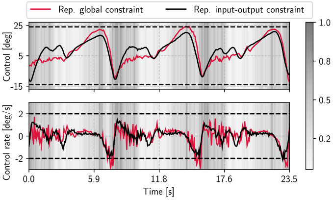
We tested NNRepLayer on the last and the second to the last layer of network policy to satisfy the constraints with a subset of the original training data including both adversarial and non-adversarial samples. In all experiments, we used samples in NNRepLayer and a held out set of size for testing. Finally, the repaired policies to satisfy global and input-output constraints are tested on a prosthetic device for minutes of walking, see Fig. 4. More specifically, the same healthy subject was fitted with an ankle bypass; a carbon fiber structure molded to the lower limb and constructed such that a prosthetic ankle can be attached to allow the able-bodied subject to walk on the prosthesis. The extra weight and off-axis positioning of the device incline the individual towards slower, asymmetrical gaits that generates strides out of the original training distribution [18, 19]. The participant is then asked to walk again for minutes to assess whether constraints are satisfied. Adversarial samples in the repair data set are hand-labeled for fine-tuning and retraining so that the target outputs satisfy the given predicates. In fine-tuning, as proposed in [1, 4], we used the collected adversarial data set to train all the parameters of the original policy by gradient descent using a small learning rate (). To avoid over-fitting to the adversarial data set, we trained the weights of the top layer first, and thereafter fine-tuned the remaining layers for a few epochs. The same hand-labeling strategy is applied in retraining, except that a new policy is trained from scratch for all original training samples. In both methods, we trained the policy until all the adversarial samples in the repair data set satisfy the given predicates on the network’s output. Our code is available on GitHub: https://github.com/k1majd/NNRepLayer.git.
C.2 Experiments and Results
Global Constraint.
The global constraint ensures that the prosthesis control, i.e., , stays within a certain range and never outputs an unexpected large value that disturbs the user’s walking balance. Additionally, the prosthetic device we utilized in these scenarios contains a parallel compliant mechanism. As such, either the human subject or the robotic controller could potentially drive the mechanism into the hard limits, potentially damaging the device. In our walking tests, see Fig. 4, we therefore specified global constraints such that the ankle angle stays within the bounds of [deg] regardless of whether it is driven by the human or the robot. In simulation experiments. see Fig. 5 (a), we enforced artificially strict bounds on the ankle angle to never exceed [deg] which is a harder bound to satisfy.
Conditional Constraint.
Depending on the ergonomic needs and medical history of a patient, the attending orthopedic doctor or prosthetist may identify certain body configurations that are harmful, e.g., they may increase the risk of osteoarthritis or musculoskeletal conditions [20, 21]. Following this rationale, we define a region of joint angles space that should be avoided. An example of such a region is demonstrated in Fig. 6 as a grey box in the joint space of ankle and femur angles.

To satisfy this constraint the control rate should be tuned such that the joint ankle and femur angles stay out of set . This constraint can be defined as an if-then-else proposition which can be formulated as the disjunction of linear inequalities on the network’s output. Figure 6 demonstrates the output of new policy after repairing with NNRepLayer. As it is shown, our method avoids the joint ankle and femur angles to enter the unsafe region . Finally, we observed that repairing the last layer does not result in a feasible solution.
Comparison w\Fine-tuning, Retraining, and REASSURE.
Table 2 better illustrates the success of our method in satisfying the constraints while maintaining the control performance. As shown in Table 2, retraining and NNRepLayer both perform well in maintaining the minimum absolute error and the generalization of constraint satisfaction to the unseen testing samples for global and input-output constraints. However, the satisfaction of if-then-else constraints is challenging for retraining and fine-tuning as the repair efficacy is dropped by almost using these techniques. It also highlights the power of our technique in generalizing the satisfaction of conditional constraints to the unseen cases.
NNRepLayer REASSURE [6] RT [s] MAE RE [%] IB [%] RT [s] MAE RE [%] IB [%] Global Input-output Conditional Infeasible Infeasible Infeasible Infeasible Fine-tune Retrain RT [s] MAE RE [%] IB [%] RT [s] MAE RE [%] IB [%] Global Input-output Conditional
C.3 Testing Repair on Larger Networks
To demonstrate the scalability of our method, we conducted a repair experiment on a network with 256 neurons in each hidden layer. We used 1000 samples for repair and 2000 samples for testing. We formulate this problem in MIQP and run the program on a Gurobi [22] solver. We terminated the solver after 10 hours and report the best found feasible solution. Figure 7 and Table 3 show the control signal, and the statistical results of this experiment, respectively. As demonstrated, our technique repaired a network with up to 256 nodes with 100% repair efficacy in 10 hours. Similar network structure and sizes are frequently used in robotics and controls tasks. Examples include [23] (3 hidden layer, 256 nodes), [24] (2 hidden layer, 64 nodes), [25] (2 hidden layer, 200 nodes), [26] (2 hidden layer, 50 nodes), and [27] (2 hidden layer, 50 nodes).
Network Size Number of Samples MAE Repair Efficacy [%] Runtime [h] Input-output Constraint 256 1000 0.62 100 10
C.4 Heuristics for Computational Speedups of NNRepLayer
In this section we provide examples for computational speedups and heuristics that lead to faster neural network repair. To this end, we repaired randomly selected nodes of a single hidden layer in a network with 64 hidden nodes for 35 times. We let the solver run for 30 minutes in each experiment (versus the full repair that is solved in 6 hours). Figure 8 demonstrates the mean absolute error (MAE), the total number of repaired weights, repair efficacy, and the original MIQP cost. Here, to detect the sparse nodes that can satisfy the constraints, we solved the original full repair by adding the norm-bounded error of repaired weights with respect to their original values to the MIQP cost function. The bold bars in Fig. 8 demonstrate the results of repairing the randomly-selected sparse nodes. Repairing of the obtained sparse nodes reached a cost value very close to the cost value of the originally full repair problem ( versus ), in only 30 minutes versus 6 hours. As illustrated, repair of some random nodes also results in infeasibility (blank bars) that shows these nodes cannot repair the network. In our future work, we aim to explore the techniques such as neural network pruning [28, 29] to select and repair just the layers and nodes that can satisfy the constraints instead of repairing a full layer. Our results in this experiment show that repairing partial nodes can significantly decrease the computational time of our technique.