Imaging the crustal and upper mantle structure of the North Anatolian Fault: A Transmission Matrix Framework for Local Adaptive Focusing
Abstract
Imaging the structure of major fault zones is essential for our understanding of crustal deformations and their implications on seismic hazards. Investigating such complex regions presents several issues, including the variation of seismic velocity due to the diversity of geological units and the cumulative damage caused by earthquakes. Conventional migration techniques are in general strongly sensitive to the available velocity model. Here we apply a passive matrix imaging approach which is robust to the mismatch between this model and the real seismic velocity distribution. This method relies on the cross-correlation of ambient noise recorded by a geophone array. The resulting set of impulse responses form a reflection matrix that contains all the information about the subsurface. In particular, the reflected body waves can be leveraged to: (i) determine the transmission matrix between the Earth’s surface and any point in the subsurface; (ii) build a confocal image of the subsurface reflectivity with a transverse resolution only limited by diffraction. As a study case, we consider seismic noise (0.1-0.5 Hz) recorded by the Dense Array for Northern Anatolia (DANA) that consists of 73 stations deployed for 18 months in the region of the 1999 Izmit earthquake. Passive matrix imaging reveals the scattering structure of the crust and upper mantle around the NAFZ over a depth range of 60 km. The results show that most of the scattering is associated with the Northern branch that passes throughout the crust and penetrates into the upper mantle.
I Introduction
The North Anatolian Fault zone (NAFZ) is one of the major continental right-lateral strike slip faults, and forms a border between the Eurasian continent and the Anatolian block. With an extremely well developed surface expression, it is one of the most active faults in the Eastern Mediterranean region (Sengör 1979; Barka 1992). It is over km long and extends from eastern Turkey in the east to Greece in the west and, historically, has been subject to many destructive earthquakes (Ambraseys and Finkel 1995; Stein et al. 1997). The seismic activity of such large faults constitutes a continuous hazard/threat to the surrounding regions and big cities, especially Istanbul city located to the West of the fault.
Faults are well defined at the surface by the localized deformation and displacement delineating the fault traces, but their deep structure remains poorly understood (Vauchez et al. 2012). The understanding of such major fault systems and seismic hazard requires a characterization of the geometrical and seismic properties of the crust and upper mantle. A large number of geological and geophysical studies have discussed the complexity of fault zones and their relation with their deep roots (Stein et al. 1997). They are not only confined in the mid crust; indeed, models suggest that they penetrate deep into the crust and extend to the upper Mantle (Lyakhovsky and Ben-Zion 2009). If so, faults develop into shear zones, corresponding to a volume of localized deformation accounting for the relative displacement of the tectonic blocks.
Seismic imaging techniques, especially reflection, refraction, and tomographic methods, constitute a very powerful tool to characterize fault zones and report the variation of the properties of the crust and the upper mantle. They rely on the study of wave propagation inside the Earth that is governed by the density and elastic properties of the rocks. To properly probe the medium, waves should be generated by a dense distribution of seismic sources. Conventional seismic exploration techniques use either earthquakes as seismic sources, or explosions and vibrators to generate seismic waves in regions with weak seismicity. Because of the limitations in the earthquake distribution and high cost of active methods, there is a need for alternative imaging approaches that would not rely on any coherent source. In the 2000’s, the extraction of deterministic information about the Earth structure from ambient seismic noise revolutionized the field of seismology (Campillo and Roux 2014, see e.g.). It was shown that the cross-correlation of diffuse waves or ambient seismic noise recorded at two stations provides an estimate of the Green’s function between those two stations (Campillo and Paul 2003, see e.g.). The reflection response of the medium is then retrieved and can be applied to build tomographic or structural images of the Earth. Because ambient noise is dominated by surface waves, their Green’s function component can be easily extracted (Shapiro and Campillo 2004). It has been demonstrated that, under energy equipartition, body wave reflections can also be retrieved from ambient seismic noise cross-correlations (Draganov et al. 2007; Poli et al. 012a; Poli et al. 012b). Body waves contain valuable information on the structure of the medium in depth and can be investigated to obtain high-resolution images of the crust and the mantle (Retailleau et al. 2020).
Faults are usually imaged indirectly through strong velocity contrasts in tomographic profiles (Zigone et al. 2019), or through the offset of geological layers observed in reflectivity images (Qian and Liu 2020). However, tomographic images exhibit a relatively poor resolution, while reflection imaging methods are strongly sensitive to the available velocity model. Interestingly, a reflection matrix approach has been recently proposed to cope with these issues. Originally developed in acoustics (Lambert et al. 020a; Lambert et al. 020b) and optics (Kang et al. 2017; Badon et al. 2020), this approach has been recently applied to passive seismology (Blondel et al. 2018; Touma et al. 2021). By considering high frequency seismic noise (- Hz), high resolution images of complex areas, such as volcanoes (Giraudat et al. 2021) and fault zones (Touma et al. 2021), have been obtained over a few km depth. In this paper, we aim to characterize the crustal structure of the NAFZ at a much larger scale (until km depth). To that aim, a lower frequency bandwidth (- Hz) has been considered. At the corresponding wavelengths, the subsurface reflectivity can be considered as continuous rather than being seen as a discrete distribution of scatterers as in our previous works (Giraudat et al. 2021; Touma et al. 2021). As we will see, this continuous reflectivity can be exploited to enable a local and adapted auto-focus on each part of the subsurface image, thereby showing an important robustness to the inaccuracy of the initial wave velocity model.
Seismic matrix imaging is based on the passive measurement of the reflection matrix associated with a network of geophones. It contains the set of impulse responses between each pair of geophones extracted from cross-correlations of seismic noise. Based on the available velocity model, a focused reflection (FR) matrix is built by applying a redatuming process to (Blondel et al. 2018; Lambert et al. 020a). This matrix contains the impulse response between virtual sources and receivers synthesized inside the medium. In the following, matrix “input” and “output” will refer to virtual sources (downgoing waves) and receivers (upgoing waves), respectively. This FR matrix is powerful as it first provides an image of the subsurface reflectivity by considering its diagonal elements (i.e when virtual source and receiver coincide); this is the so-called confocal image. Moreover, its off-diagonal elements allow a local quantification of aberrations in the vicinity of each virtual source. Those aberrations correspond to the imperfections of the image induced by the mismatch between the wave velocity model and the actual seismic velocity distribution in the subsurface. In contrast with previous works (Giraudat et al. 2021; Touma et al. 2021), a multi-layered wave velocity model is here considered rather than just an homogeneous model. This more sophisticated description of seismic wave propagation enables a better time-to-depth conversion in the confocal image and a better focusing process. Nevertheless, the FR matrix still highlights residual aberrations that result from the mismatch between the velocity model and the actual velocity distribution. The fluctuations of wave velocities actually induce phase distortions on the focused wave-fronts that result in a blurry image of the NAFZ subsurface.
To overcome these detrimental effects, the FR matrix can be first projected in a plane wave basis. By exploiting the angular input-output correlations of the reflection matrix, phase distortions of the incident and reflected wave-fronts can be identified and compensated. This is the principle of the CLASS algorithm (acronym for closed-loop accumulation of single scattering), originally developed in optical microscopy (Kang et al. 2017; Choi et al. 2018; Yoon et al. 2020). Applied for the first time to seismology in the present study, CLASS successfully compensates for spatially-invariant aberrations and will be shown to clearly improve the confocal image of the NAFZ subsurface.
Nevertheless, high-order aberrations subsist and are addressed through the distortion matrix concept in a second step. Originally introduced in ultrasound imaging (Lambert et al. 020b) and optical microscopy (Badon et al. 2020), this operator contains the phase distortions of the incident and reflected wave-fronts with respect to the propagation model. It was recently exploited in passive seismology in order to image the San Jacinto Fault zone scattering structure that exhibits a sparse distribution of scatterers (Touma et al. 2021). Here, we apply it in a new scattering regime since the NAFZ subsurface exhibits, in the frequency range under study, a continuous reflectivity distribution made of specular reflectors and randomly distributed heterogeneities. In this regime, a local time reversal analysis of the distortion matrix can be performed in order to retrieve the transmission matrix between the Earth’s surface and any point of the subsurface (Lambert et al. 022b). This transmission matrix is a key tool since its phase conjugate provides the optimized focusing laws that need to be applied to the reflection matrix in order to retrieve a diffraction-limited image of the subsurface. While most conventional reflection imaging techniques are strongly sensitive to the available velocity model, the reflection matrix approach is robust with respect to its limitations. An approximate velocity distribution is actually sufficient since a time-reversal analysis of seismic data enables a local and adapted auto-focus on each part of the subsurface image.
To image the crustal structure of NAFZ, we use data from the Dense Array for Northern Anatolia (DANA 2012) that was deployed over the western segment of the fault, in the latest rupture region during the 1999 Izmit () and Düzce () earthquakes (Barka et al. 2002; Akyuz et al. 2002). The dense array was installed temporarily between May 2012 and October 2013. It consists of 73 3-component broadband seismometers, 66 stations arranged along east-west lines and 6 North-South lines forming a rectangular grid and covering an area of km by km with a nominal inter-station spacing of 7km (Fig. 1a). Seven additional stations were deployed east of the rectangular array in a semi-circle shape. In this region, the fault splits into two major strands: the northern (NNAFZ) and southern (SNAFZ) strands (Fig. 1b). The northern strand, where most of the continuous deformation occurs according to geodetic studies (Barka 1992; Reilinger et al. 2006), has been subject to a series of major earthquakes in the last century, among them the 1999 Izmit Earthquake. On the contrary, the latest rupture of the southern branch dates back to the fifteenth century (Ambraseys 2002). The fault delineates three tectonic blocks (Fig. 1b): (i) the Istanbul Zone (IZ) situated North of the northern branch, (ii) the Sakarya zone (SZ) situated to the South of the southern branch and (iii) the Armutlu-Almacik crustal block (AA) located in the center, between the two fault strands (Yılmaz et al. 1995; Okay and Tüysüz 1999; Chen et al. 2002). Differences in crustal composition and properties between these blocks have been reported. Strong velocity contrasts were found across the fault strands by several tomographic studies (Salah et al. 2007; Koulakov et al. 2010; Papaleo et al. 2017; Papaleo et al. 2018) and full waveform inversion studies (Fichtner et al. 2013; Çubuk-Sabuncu et al. 2017). Low velocity zones are found below the surface traces of the SNAFZ and NNAFZ (Papaleo et al. 2017; Papaleo et al. 2018). The crust of Istanbul and Armutlu Blocks is characterized by high velocities while SZ shows relatively low velocities (Koulakov et al. 2010; Papaleo et al. 2017; Papaleo et al. 2018; Taylor et al. 2019).
The present study reveals the 3D scattering structure of the medium below this major fault. It does not only image planar interfaces, but provides a direct insight on the heterogeneities that mainly sit in the vicinity of the strands. The observed results complement previous studies conducted in the region. A step in the Moho is detected below the Northern branch, and several sub-Moho structures are observed in the North confirming that the northern branch penetrates in the upper mantle. The southern strand does not have a strong signature in the scattering profiles.
II Passive Seismic Matrix Imaging
II.1 Reflection matrix in the geophones basis
To apply matrix imaging, we used the ambient seismic noise recorded at DANA (see Fig. 1) to compute the cross-correlation functions of horizontal EE component over the 18 months of recording period. The choice of the EE component is made because it displays a better signal-to-noise than the NN component. With this choice of body wave component, the waves being dealt with are mostly shear waves that have been reflected in depth. First, the data were down-sampled at Hz and corrected from instrument response. Then, the data were split into one-hour windows. Each window is band-pass filtered between and Hz after applying a spectral whitening between and Hz (Bensen et al. 2007). The cross-correlation between each pair of stations is computed over one-hour windows and finally stacked to obtain the mean cross-correlation function with time lags ranging from to s. The causal and the anti-causal parts of the cross-correlations are then summed in order to improve the convergence towards the Green’s functions between seismic stations. Although, considering seismic noise in a higher frequency range would allow, in principle, to improve the resolution of the images, matrix imaging requires the Nyquist criterion to be fulfilled: The inter-station distance ( km) shall be of the order of a half-wavelength. Considering a S-wave velocity m/s near the surface, this criterion led us to choose the Hz frequency range ( km at the central frequency, with the wavelength at the Earth surface). The ambient noise energy in the frequency band considered in this study comes from the secondary microseisms ( s period band) produced in the ocean (Longuet-Higgins 1950; Hasselmann 1963; Stehly et al. 2006) and constitutes one of the most energetic parts of the seismic noise.

The symmetric cross-correlations can be stacked in a time-dependent response matrix . One element of this matrix corresponds to the impulse response between geophones located at positions and . In other words, contains the seismic wave-field recorded at receiver if a pulse was emitted by the virtual source at time . In the following, we will thus refer to columns and lines of the response matrix as input and output wave-fields, respectively.
Figure 1c shows the impulse responses between pairs of stations located South of the SNAF and having at least an angle of with the East-West direction because of the EE polarization considered in this study. These responses are stacked for different inter-station distances. Figure 1c is dominated by surface-wave energy travelling at about m/s. Given the horizontal polarization of seismic waves considered here, these surface waves correspond to Love waves. Interestingly, some nearly vertical weaker events are also observed at larger times. Due to their horizontal polarization, they correspond to shear waves reflected by the subsurface heterogeneities in depth.
Another way to highlight the surface and bulk wave components is to investigate the response matrix in the frequency domain. To this aim, a temporal Fourier transform is applied to . For each frequency in the bandwidth of interest (0.1-0.5 Hz), a monochromatic matrix is obtained. The different wave components can then be discriminated by a plane wave decomposition of the output wave-fields, such that
| (1) |
where the symbol stands for the standard matrix product. is the Fourier transform operator that connects each geophone’s position to the transverse wave vector of each angular component of the wave-field:
| (2) |
where the symbol denotes the scalar product. Figure 2a shows the result of this plane wave decomposition by displaying the mean angular distribution of the output wave-field at Hz. More precisely, this distribution is displayed as a function of the ratio between spatial frequencies and and frequency . In that representation, surface waves emerge along a circle whose radius should correspond to the slowness of Love waves, with m. (Taylor et al. 2019). On the other hand, reflected bulk waves are distributed over a disk of radius .
Figure 2a clearly reveals: (i) The contribution of Love waves with a dominant intensity lying along the y-direction; (ii) A bulk wave component arising at small spatial frequencies and corresponding to the nearly vertical echoes already highlighted by Fig. 1c. The latter contribution is a priori induced by extended reflectors in depth. On the contrary, diffuse scattering can generate reflected waves over a larger distribution of angles. It can therefore account for the incoherent background observed in Fig. 2a. This background could result from the averaging of the random speckle pattern exhibited by the angular distribution of the reflected wave-field when only a few sources are considered (Fig. 2b). Nevertheless, it is difficult at this stage to be more affirmative since an imperfect convergence of noise correlations could also lead to such a random wave-field.

A redatuming process is thus required to enhance the weight of scattered shear waves from seismic noise correlations and image the reflectivity of the deep structures around the NAFZ.
II.2 Redatuming process
An image of the medium reflectivity can be obtained by applying a double focusing operation to (Blondel et al. 2018; Touma et al. 2021). It consists in back-propagating the response measured at the surface into wave-fields below the surface as if there were sources and receivers inside the medium. This is similar to the ”wave-field extrapolation” concept that forms the basis of the migration process (Berkhout 1981). It requires performing beamforming operations both at emission and reception. On the one hand, focusing in emission consists in applying appropriate time delays to the emitted sources so that waves constructively interfere and focus on one point inside the medium. Physically, this operation amounts to synthesizing a virtual source inside the medium. On the other hand, focusing in reception is carried out by applying proper time delays to the received signals so that they can constructively interfere. As in emission, this focusing operation can be seen as the synthesis of a virtual receiver inside the medium. This operation is known as ”redatuming” in seismology (Berkhout and Wapenaar 1993) and consists of virtually moving sources and receivers from the surface to the medium below (Fig. 3a). Generally, an image of the sub-surface is built by considering the response of virtual source and receiver placed at the same location (Fig. 3f). On the other hand, the principle of matrix imaging consists in decoupling both locations (Lambert et al. 020a).
In the following, the reflection matrix will be expressed in three different bases: (i) the geophones basis where the matrix represents the cross-correlations between all pairs of stations located at , (ii) the focused basis corresponding to the location of virtual sources and receivers synthesized by the focusing operations and in which the image of the medium is built, and (iii) the spatial Fourier basis that will be first used for wave-field extrapolation and then for aberration correction.
II.3 Propagator from the geophones to the focused basis
The focusing operations described in section II.2 provide the FR matrix that plays a pivotal role in matrix imaging. We now show how this matrix can be obtained through simple matrix operations.
Mathematically, the response between virtual sources and receivers is obtained from the response matrix at the surface through the Green’s functions, that describe the propagation between each geophone and each point inside the medium using a wave velocity model. Switching between bases can be easily achieved by simple matrix products in the frequency domain. We first define the plane-wave propagator , that enables a direct projection of the response matrix from the geophones’ basis to the focused basis at each depth . Each monochromatic response matrix can be projected in the focused basis both at input and output by applying appropriate phase shifts associated with downgoing waves at input and upgoing waves at output to provide the FR matrix (Fig. 3a). Under a matrix formalism, this operation can be written as follows:
| (3) |
where the symbols and stands for phase conjugate and transpose conjugate, respectively.
A model for the wave velocity distribution inside the medium is required. In this study, and since the horizontal EE cross-correlation functions are considered, only an estimate of the S-wave velocity is required. Unlike Blondel et al. 2018 and Touma et al. 2021 that considered a homogeneous P-wave velocity model, here a layered 1-D S-wave velocity model is used for the focusing process. A combination of two models derived by Kahraman et al. 2015, for the first km, and by Karahan et al. 2001, for deeper layers is displayed in Table 1. Compared to an homogeneous model, such a layered model will allow better time-depth conversion and will limit the aberration level in the subsurface image. Note, however, that our wave propagation model will not account for multiple reflections that could, in principle, take place between the interfaces of the different layers.
| Layer # | Depth (km) | |
|---|---|---|
| 0 | 0 - 1 | 1700 |
| 1 | 1 - 3.5 | 2500 |
| 2 | 3.5 - 14 | 3200 |
| 3 | 14 - 26 | 3500 |
| 4 | 26 - 40 | 3600 |
| 5 | 40 - 60 | 4300 |
In a layered medium, the forward and backward extrapolation of the reflection matrix can be performed through the decomposition of the wave-field into plane waves (Berkhout 1981). Indeed, plane waves can be easily extrapolated by applying a simple phase shift. To that aim, we define the spatial transfer function, , that models the ballistic propagation of shear waves through the layer:
| (4) |
with
the vertical component of the wave vector in the layer, the wave velocity in the layer of our model and its thickness. To propagate the plane waves from the surface to depth z, we define the wave-field extrapolator, , as the product of the spatial transfer functions of the layers above the considered depth as follows:
| (5) |
where is the depth at which starts the layer. The phase propagator, , can finally be expressed as follows:
| (6) |
where the symbol refers to the Hadamard product (i.e. element wise matrix multiplication). In the equation 6, the term-by-term product arises because wave propagation in the plane wave basis is modeled by the scalar product of each plane wave component with the overall spatial transfer function . The matrix multiplication stands for the inverse Fourier transform that enables us to project the propagated wave-field from the plane wave basis to the focused basis. is actually the Fourier transform operator linking the focused and plane wave bases. It connects the transverse wave vector of each plane wave to the transverse coordinates of each focusing point:
| (7) |
To avoid aliasing during the change of basis between the plane wave and focused bases, a Shannon criterion should be respected. The transverse wave components, and , are required to fulfill the following condition:
| (8) |
The resolution of the Fourier plane is conditioned by the size of the array km such that . By properties of the Fourier transform, the transverse resolution in the focal plane, that corresponds to the distance between the focusing points , is chosen to be km to circumvent spatial aliasing in the focused basis.
As shown by Eq. 5, wave components of spatial frequencies larger than the wavenumber cannot be transmitted through the ith layer. As a consequence, redatuming acts as a low-pass filter in the spatial frequency domain. To illustrate this phenomenon, one can back-project the focused reflection matrix in the geophone basis,
| (9) |
where the superscript stands for matrix transpose. From , one can investigate the angular decomposition of the output wave-fields as previously done for the original response matrix in Figs. 2(a) and (b) (Eq. 1). The result is displayed in Figs. 2(c) and (d). The comparison with their original counterparts highlights the low pass-filter operated by redatuming: The surface wave component is discarded and only the shear waves associated with spatial frequencies are kept. Figure 2(d) displays: (i) a low-spatial frequency component associated with specular reflectors; (ii) several off-axis bright spots associated with peculiar single scattering events at depth and; (iii) a diffuse background that is difficult to interpret at this stage since it can be due to random single scattering, multiple scattering or noise resulting from the imperfect convergence of cross-correlations towards the Green’s function. To enhance the single scattering contribution with respect to the other undesirable components for imaging, the idea is now to perform a time gating operation to enhance the single scattering contribution.
II.4 Broadband focused reflection matrix
Equation 3 simulates focused beamforming for both downgoing (input) and upgoing (output) shear waves at each frequency. Each spectral component of the wave-field can then be recombined to provide a broadband focused reflection matrix :
| (10) |
with Hz and Hz. This operation amounts to performing an inverse Fourier transform at time over the frequency band [0.1 0.5] Hz. Note that this inverse Fourier transform is only performed over positive frequencies in order to have access to both the amplitude and phase of the wave-field. The time origin here corresponds to the ballistic time in the focused basis. Equation 10 thus corresponds to a time gating operation that tends to select singly-scattered waves associated with a scattering event in the focal plane. Each coefficient of contains the complex wave-field that would be recorded by a virtual geophone located at if a virtual source at emits a pulse of length at the central frequency , with Hz.
The FR matrix can be expressed theoretically as follows (Lambert et al. 020a; Lambert et al. 022a; Touma et al. 2021),
| (11) |
which yields, in terms of matrix coefficients,
| (12) |
The matrix describes the scattering process in the focused basis. In the single scattering regime, this matrix is diagonal and its coefficients correspond to the subsurface reflectivity at depth . is the focusing matrix whose coefficients correspond to the point spread functions (PSFs) of the redatuming process. These PSFs represent the spatial amplitude distribution of the focal spots for each focusing point . They thus account for the lateral extent of each vitual source/detector at .
An example of the broadband FR matrix is shown at depth km in Fig. 3b. is a four-dimension matrix concatenated in 2D as a set of blocks (Blondel et al. 2018). If the wave velocity model was correct, the PSFs of the redatuming process would be close to be point-like [, with the Dirac distribution] and the focused reflection matrix almost diagonal [, see Eq. S1]. Here, the backscattered energy is far from being concentrated along the diagonal of , which is a manifestation of the gap between our layered wave velocity model (Table 1) and the real shear wave velocity distribution in the subsurface.
II.5 Confocal image
Nevertheless, one can try to build an image of the medium reflectivity at each effective depth by considering the diagonal elements of the FR matrix, i.e where the virtual sources and receivers coincide (, see Fig. 3c). It yields the so-called confocal image:
| (13) |
Fig. 3e shows the resulting 2D image at km retrieved from the diagonal of the FR matrix in Fig. 3b. By injecting Eq. S1 into the last equation, can be expressed as the transverse convolution between the medium reflectivity and the confocal PSF , such that:
| (14) |
Such an image is thus a reliable estimator of the reflectivity at depth only if the wave velocity model is close to reality. In this ideal case, the spatial extent of the PSF is only limited by diffraction and the transverse resolution is given by (Born and Wolf 2003):
| (15) |
where is determined by the size of the array km, and corresponds to the maximum angle under which a focusing point sees the geophones’ array.
By stacking the confocal image computed at each depth , a 3D image of the reflectivity can be obtained. The cross-section at Lon is displayed in Fig. 4a. 2D confocal images at and km are also shown in Fig. 4b. Unlike the transverse resolution, the axial resolution is limited by the frequency bandwidth: km, with the shear wave velocity at the considered depth. The sections of the 3D image displayed in Figs. 3e, 4a and 4b show a greater reflectivity in the central part of the field-of-view, i.e right below the geophones’ array, but no direct correlation can be found between the image and the location of the fault strands. In fact, as we will see now, lateral wave speed heterogeneities strongly degrade the transverse resolution of the redatuming process and induce strong aberrations in the confocal image. This image is thus not a reliable estimator of the medium reflectivity at this stage and cannot be interpreted.

II.6 Quantification of aberrations
The FR matrix can provide more than a confocal image since its off-diagonal elements can lead to a quantification of aberrations. To that aim, a relevant observable is the distribution of the backscattered intensity around a common midpoint point as a function of the relative position, , between the input and output focusing points (Lambert et al. 020a; Touma et al. 2021):
| (16) |
In the following, we will refer to this quantity as the reflection point spread function (RPSF).
To express this quantity theoretically, we first make a local isoplanatic approximation in the vicinity of each point (Lambert et al. 022a). Isoplanicity means here that waves which focus in this region are assumed to have travelled through approximately the same areas of the medium, thereby undergoing identical phase distortions. The PSF can then be considered to be spatially invariant within this local region. Mathematically, this means that, in the vicinity of each point , the spatial distribution of the PSF, , only depends on the relative distance between the point and the focusing point . This leads us to define a local spatially-invariant PSF around each common mid-point such that:
| (17) |
Under this local isoplanatic assumption, the RPSF can be derived analytically in different scattering regimes. On the one hand, for large reflectors such as horizontal interfaces between geological units, the medium reflectivity can be assumed as locally constant and the RPSF is given by (see Supplementary Section S1):
| (18) |
where the symbol denotes convolution. On the other hand, for diffuse scattering, the medium reflectivity can be considered, in first approximation, as randomly distributed. Under that assumption, the mean RPSF is then proportional to the convolution between the incoherent output and input local PSFs, independently from the medium’s reflectivity (Lambert et al. 020a) (see Supplementary Section S1):
| (19) |
where the symbol stands for an ensemble average. Whatever the scattering regime, the spatial extension of the RPSF is thus roughly equal to the lateral dimension of the PSF. If we assume a Gaussian PSF, this equality is strict. The RPSF is thus a direct indicator of the focusing quality and its spatial extent directly provides an estimation of the local transverse resolution of the confocal image.
Fig. 3c displays the RPSF averaged over the whole field-of-view at depth km. For sake of comparison, Fig. 3d shows the ideal (i.e diffraction-limited) RPSF that would be obtained in absence of aberrations. The comparison between Figs. 3c and d highlights the impact of aberrations resulting from the mismatch between the wave velocity model of Table 1 and the real wave speed distribution. Indeed, the full width at half maximum of the intensity profile is increased by a factor compared to its diffraction-limited value (white circle in Fig. 3d, Eq. 15) at depth km. This effect explains the blurred aspect of the confocal image displayed in Fig. 3e at the same depth. The impact of aberrations is also illustrated in by Fig. 4c that displays the depth evolution of the RPSF inside the Earth. As with the diffraction-limited resolution (Eq. 15), the transverse extension of the RPSF also increases with but it shows a much larger extension.
In the following we will show how matrix imaging can restore an optimal resolution for this image.
III Exploiting the input-output angular correlations of the wave-field: The CLASS algorithm
In order to compensate for aberrations, the reflection matrix can be first projected in the plane wave basis:
| (20) |
Using Eq. 7, the last equation can be rewritten, in terms of matrix coefficients, as a double spatial Fourier transform:
| (21) |
Each coefficient of the matrix thus contains the medium response between input and output transverse wave vectors and . By injecting Eq. 11 into Eq. 20, the matrix can be expressed as follows:
| (22) |
where is the transmission matrix describes plane wave propagation between the focused and the plane wave bases. Its coefficients correspond to the angular decomposition of the wave-field produced at the Earth surface for a point-like virtual source located at . This matrix is critical for imaging since its inversion can provide a direct access to the subsurface reflectivity, without relying on a precise wave velocity model.
As a first step towards the estimation of , we can go one step further in the isoplanatic approximation (Eq. 17) by assuming a full transverse-invariance of the PSF across the field-of-view. This leads us to define a laterally-invariant PSF , such that:
| (23) |
This strong assumption means that wave speed heterogeneities are modelled by a phase screen of transmittance in the plane wave basis, such that , where is the Fourier transform of the spatially-invariant PSF . The aberration transmittance grasps the phase distortions undergone by downgoing and upgoing wave-fields during their travel between the Earth surface and the focal plane at effective depth .
Under this full isoplanatic approximation (Eq. 23), a theoretical expression of can be derived in the single scattering regime (Lambert et al. 020b):
| (24) |
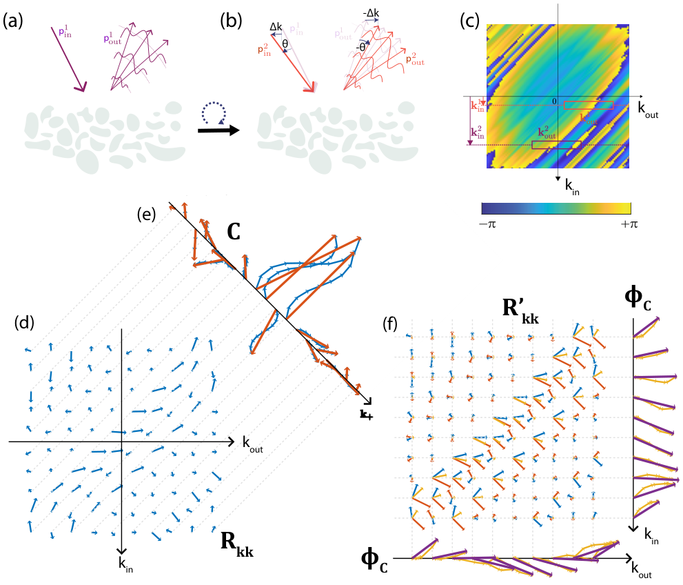
where is the 2D Fourier transform of the medium’s reflectivity at each depth . In absence of aberrations , the reflection matrix expressed in the plane wave basis exhibits a deterministic coherence along its antidiagonals (=constant, see Fig. 5c): (Aubry and Derode 2009; Kang et al. 2015). This peculiar property is a manifestation of a phenomenon called the memory effect in wave physics (Freund et al. 1988; Shahjahan et al. 2014). When an incident plane wave () illuminates a scattering medium, it gives rise to a reflected wave-field () that exhibits a speckle feature (Fig. 5a) due to the random interference between partial waves induced by each scatterer lying at depth . When this incident plane wave is rotated by a certain angle (), the reflected wave-field is tilted in the opposite direction (, see Fig. 5b). This correlation between the downgoing and upgoing wave-fields accounts for the deterministic coherence along the antidiagonals of (Fig. 5c). However, in the present case, this property is not checked because of the phase distortions undergone by downgoing and upgoing wave-fields induced by wave speed heterogeneities. Mathematically, this is accounted by the phase screen in Eq. 24 that breaks the correlation between coefficients lying along the same antidiagonal (Fig. 5d).
The principle of the CLASS algorithm (Kang et al. 2017; Choi et al. 2018; Yoon et al. 2020) consists in restoring this coherence by applying a phase correction , , to the input and output of :
| (25) |
where is the estimator of the aberration phase law whose phase conjugate maximizes the coherence along the antidiagonals of . To compute , the first step is to perform a coherent sum of ’s coefficients along each of its antidiagonals [see Fig. 5e]:
| (26) |
with . As shown in Supplementary Section S2, is a rough estimator for the spatial frequency spectrum of the medium reflectivity (see Supplementary Section S2). The second step consists in performing the Hadamard product (element-wise product) between the phase conjugate of the vector and the matrix (Fig. 5f):
| (27) |
The last operation amounts to compensate for the phase fluctuations of the reflectivity spatial frequency spectrum in . The isoplanatic phase distortion is finally estimated by summing the columns of the compensated matrix (see Fig. 5f)
| (28) |
The phase conjugate of the resulting wave-front, , tends to realign in phase the coefficients lying on the same antidiagonal of (Eq. 25). As shown in Supplementary Section S2, this phase realignment in the plane wave basis is equivalent to a maximization of the confocal intensity in the focused basis.
The corresponding FR matrix can be deduced as follows:
| (29) |
A corrected confocal image is extracted from the diagonal of and displayed in Fig. 6a at depth km . It should be compared with the original image shown in Fig. 3e. While the latter one displays a random-like feature, the corrected image reveals a greater reflectivity in the North that can be correlated with the expected damage around the Northern branch of the fault. The comparison between these two images illustrates the benefit of the correction process. The gain in resolution can be assessed by averaging the RPSF (Eq. S2) over the whole field-of-view (see Fig. 6c). Compared to the original RPSF displayed in Fig. 3c, we can notice that a large component of the off-diagonal energy has been brought back to the confocal lobe (white circle). The resolution is reduced from km to km but it is still larger than the diffraction-limited resolution ( km at the considered depth). A diffuse component subsists and can be explained by the spatially-varying residual aberrations, , that have not been compensated by the CLASS algorithm, such that .
A local compensation of higher order aberrations is thus required. This issue is handled in the following section by investigating the reflection matrix and its distorted component between the focused and plane wave bases.

IV Matrix approach for adaptive focusing: The local distortion matrix
The distortion matrix was already introduced in ultrasound (Lambert et al. 020b; Lambert et al. 022b), optics (Badon et al. 2020; Najar et al. 2023) and seismology (Touma et al. 2021). Several applications proved the efficiency of this matrix in overcoming aberrations and improving the image quality. Recent works in seismology (Touma et al. 2021) and optics (Badon et al. 2020) have shown that for certain scattering regimes (specular reflectors or sparse scattering), there was a one-to-one association between the eigenstates of and the isoplanatic patches present in the field-of-view. Here, this property does not hold because the NAFZ subsurface exhibits a continuous but fluctuating reflectivity (see Supplementary Section S3). In this scattering regime, local distortion matrices should be considered over restricted areas in which the isoplanatic hypothesis is ideally fulfilled (Lambert et al. 022b; Najar et al. 2023).
In this section, the distortion matrix concept is applied to the CLASS FR matrix obtained in the previous section for compensation of spatially-distributed aberrations. The process is outlined by five steps: (i) projection of the CLASS FR matrix at output into the plane wave basis (Fig. 7a), (ii) the realignment of the reflected wave-fronts to form a distortion matrix (see Fig. 7b), (iii) the truncation of into local distortion matrices , (iv) the singular value decomposition of to extract a residual aberration phase law for each point and build an estimator of the transmission matrix (Fig. 7c); (v) the phase conjugation of to correct for output residual aberrations (Fig. 7d). All of these steps are then repeated by exchanging output and input bases.
IV.1 The distortion matrix
The output of the CLASS algorithm is a focused reflection matrix that still exhibits laterally-varying aberrations. To assess these residual aberrations, the first step is to chose a basis in which the distortion of the CLASS wave-front is the most spatially-invariant. In a horizontally multi-layered medium such as NAFZ, the plane-wave basis is the most adequate since plane waves are the propagation invariants in this geometry. A plane-wave projection is performed at the output of the CLASS FR matrix :
| (30) |
connects each input focusing point to the CLASS wave-field in the plane wave basis (Fig. 7a).
The CLASS wave-field can be understood as a sum of two components: (i) a geometrical component described by the reference matrix , containing the ideal wave-front generated by a source at according to the propagation model described in Table 1 (dashed black curves in Fig. 7a ); (ii) a distorted component due to spatially distributed aberrations that subsists after the CLASS procedure. The latter component refers to the residual phase distortions that should be isolated from the CLASS wave-field in order to be properly compensated. This can be done by subtracting the ideal wave-front that would be obtained in absence of aberrations (i.e the geometrical component) from each CLASS wave-front induced by each input focusing wave at . Such operation can be expressed mathematically via a Hadamard product between and . It yields the residual distortion matrix :
| (31) |
The matrix connects any input virtual source to the residual distortion exhibited by the CLASS wave-field expressed in the plane wave basis (Fig. 7b). By removing the geometrical component of the CLASS wave-field, spatial correlations are highlighted between distorted wave-fields induced by neighbour virtual sources (Badon et al. 2020). Such correlations are a manifestation of a spatial invariance of residual aberrations over areas generally referred to as isoplanatic patches (Lambert et al. 022b).
IV.2 Local distortion matrices
Our strategy is to divide the field-of-view into a set of overlapping regions (Fig. 6d). Each region is defined by a central midpoint and a spatial extension . For each region, the local residual -matrix is defined as:
| (32) |
where is a spatial window function such that for and , and zero elsewhere. Ideally, wave-front distortions should be invariant over each region, meaning that the virtual sources associated with each region belong to the same isoplanatic patch. However, in practice, this hypothesis is not fulfilled. The isoplanatic length actually scales as the typical transverse dimension over which the wave velocity fluctuates. On the one hand, the dimension of the window function should therefore be reduced to cover the smallest isoplanatic region as possible in order to provide a local and sharp measurement of aberrations. On the other hand, it should also be large enough to include a sufficient number of realizations of disorder in order to unscramble the effect of aberrations from the medium’s reflectivity (Lambert et al. 022b). To reach a good estimate of the aberration phase law, the number of input focusing points in each region should be one order of magnitude larger than the number of resolution cells mapping the CLASS focal spot (Fig. 6c) (Lambert et al. 020b). This is why the initial CLASS step was important to initiate the aberration correction process and reduce the extension of the focal spots before a local and finer compensation of residual aberration by means of the -matrix concept. The area covered by the CLASS focal spot being (Fig. 6c), the extent of the window is chosen to be .
IV.3 Singular value decomposition
Assuming local isoplanicity in each spatial window (Eq. 17), the coefficients of each distortion matrix matrix can be expressed as follows (Lambert et al. 020b):
| (33) |
This equation can be seen as a product between two terms: the output aberration transmittance and a virtual source term modulated by the medium’s fluctuating reflectivity . The goal is now to unscramble these two terms in order to get a proper estimation of the aberration transmittance at each point .
In practice, this can be done through a singular value decomposition (SVD) of each local distortion matrix :
| (34) |
where is a diagonal matrix containing the real positive singular values in a decreasing order . and are unitary matrices whose columns, and , correspond to the output and input singular vectors, respectively. The physical meaning of this SVD can be intuitively understood by considering the asymptotic case of a point-like input focusing beam: . In this ideal case, Eq. 33 becomes: . Comparison with Eq. 34 shows that, a first approximation, is of rank 1. The first output singular vector yields the residual aberration transmittance while the first input singular vector directly provides the medium reflectivity over the spatial window .
However, despite the CLASS correction, the input PSF remains far from being point-like (Fig. 6c). The spectrum of then displays a continuum of singular values but the first eigenstate of is still of interest. corresponds to a rough estimate of the medium reflectivity that allows realignment in phase for each input focal spot. Therefore, the SVD process allows the synthesis of a coherent virtual reflector that can be leveraged for the estimation of the residual aberration transmittance (Fig. 7c). More precisely, this is the normalized output singular vector , that constitutes a relevant estimator for (Lambert et al. 022b). The estimator of the transmission matrix is then given by the Hadamard product:
| (35) |
with , the phase of . The phase conjugate of provides the focusing laws to compensate for the output phase distortions over each patch (Fig. 7d). The same method can be repeated by exchanging the focused and Fourier bases between input and output in order to estimate the transmission matrix (Lambert et al. 022b). The whole process is iterated once to refine the estimation of and .
IV.4 Transmission matrix estimator
The input phase laws obtained at the end of the aberration correction process are displayed in Fig. 6e for the central regions of the field-of-view highlighted in Fig. 6d. Although they show some similar features (in particular the low spatial frequency components), they also display some differences that are quantified by the correlation coefficient between the different phase masks with the central one. The value of this coefficient is reported below each phase mask. This correlation coefficient goes from for the closest spatial windows to for the furthest ones. One can also notice that clear differences in the phase behaviour can be observed between the north, center and the south of the field-of-view. The presence of these lateral differences is consistent with the three geological blocks in the region (Fig. 1b). The latter observation together with the correlation coefficient value show the importance of estimating a different phase law for each area and justifies the implementation of a local aberration correction process.
IV.5 Local compensation of spatially-distributed aberrations
Using and , a corrected FR matrix can be finally obtained:
| (36) |
The corresponding confocal image and RPSF are displayed at km in Figs. 6(d) and (f). The comparison with their CLASS counterparts [Figs 6(a) and (c)] shows the importance of the local matrix analysis. The diffuse background is clearly reduced and the RPSF is nearly similar to its ideal value (Fig. 3d), with almost all the backscattered energy contained in the white circle accounting for the diffraction limit. The residual background in Fig. 6f is probably associated with high-order aberrations whose coherence length (isoplanatic area) is smaller than the size of the window function .
| Correction steps | 0 | 1 | 2 | 3 | 4 | 5 | 6 |
| Correction type | 0 | CLASS | CLASS | D | D | D | D |
| Correction side | Output | Input | Output | Input | Output | Input | |
| Confocal gain (dB) | 2.41 | 5.17 | 7.1 | 9 | 9.16 | 9.26 | |
| Resolution (km) | 40 | 20 | 8 | 7 | 6 | 6 | 6 |
To be more quantitative, a confocal gain can be computed from the intensity ratio between the corrected (Fig. 6a and d) and initial (Fig. 3e) images. The transverse resolution can also be estimated from the full width at half maximum of the RPSF. The confocal gain and the resolution are reported in Table 2 at each step of the aberration correction process for depth km. Strikingly, the transverse resolution is enhanced by a factor compared with its initial value and the confocal intensity is increased by more than 9 dB. These values highlight the benefit of matrix imaging for in-depth probing of NAFZ at a large scale.
In the next section, the 3D image of the medium around the NAFZ is now revealed by combining the images derived at each depth. A structural interpretation is then provided in light of previous studies on the NAFZ.
V 3D structure of the NAFZ

The previous sections have shown the process for a local compensation of phase distortions. Performing this correction process at each depth allows to uncover a well-resolved 3D image of the subsurface.
Figure 8a shows a North-South cross-section from the final 3D image. This cross-section is chosen at the same location as the one in Fig. 4a and crosses the two fault strands. It also spans the three geological units: Istanbul zone (IZ), Armutlu-Almacik (AA) and Sakarya zone (SZ). The scattering generated by the heterogeneities of the medium induce a decrease of the backscattered energy with depth. Consequently, a drop of amplitude is observed in the 3D images. In order to compensate for this, the intensity in the cross-sections is normalized by the mean intensity calculated at each depth.
Three depth slices retrieved from the final 3D images at and km are also represented in Fig. 8b with their corresponding RPSFs in Fig. 8c. Compared to the initial RPSFs (Figs. 4c), the resolution is significantly improved by a factor that increases from at small depth ( km) to beyond km. The final matrix images in Fig. 8b can also be compared to the initial confocal ones in Fig. 4b. While the original images show random-like features, the images obtained after aberration correction reveal better defined features and a reflectivity that is mainly concentrated in the North. The same observation can be made by looking at the corrected cross-section in Fig. 8a. The differences between the corrected and raw cross-sections are pronounced. While in the raw image, no clear structures and layers are visible, the corrected image reveals sub-horizontal structures with a refined level of details, thanks to the drastic gain in resolution revealed by the RPSF.
Due to its significant seismic activity over the past 100 years, and to assess the ongoing hazard posed by this activity, extensive research has been conducted on the NAFZ to image its structure and determine its mechanical characteristics. The scattering structure in Fig. 8a is interpreted with reference to prior studies conducted in the region.
The first thing to notice in the profiles is that the scattered energy is predominantly situated in the North, which corresponds with the location of the Northern branch. This observation may be associated with the greater seismic activity of the Northern strand compared to the seismic activity of the Southern strand. The scattering below this strand and to the North of it, that extends to at least km, can be explained by the damage caused by the large deformation of this complex fault system with a cumulative slip of the order of km (Armijo et al. 1999; Bohnhoff et al. 2016) during the last million years as well as the heterogeneities that have been inherited from the complex tectonic history of the region.
At the east of the Sea of Marmara, the Moho depth was reported to be between and km (Zor et al. 2003; Vanacore et al. 2013). A deepening of the Moho was identified ( km) in the IZ by Frederiksen et al. 2015, Taylor et al. 2016, Papaleo et al. 2017, Papaleo et al. 2018, Rost et al. 2021 and Jenkins et al. 2020. In Fig. 8a, a high scattering zone is observed between and km depth corresponding to a heterogeneous lower crust. Its lower boundary indicates the presence of the Moho (red dashed line). The Moho depth varies from km in the South to km in the North. The reflectivity is disrupted around N suggesting the presence of a step in the Moho below the Northern strand. The latter observation is in agreement with previous studies (Rost et al. 2021; Jenkins et al. 2020). Below the Moho, reflective structures are observed, mainly beneath AA and IZ, in agreement with Kahraman et al. 2015. These findings, supported with other studies (Kahraman et al. 2015; Papaleo et al. 2018; Jenkins et al. 2020; Rost et al. 2021), suggest that the NNAF cuts though the entire crust and reaches the upper mantle (Kahraman et al. 2015; Papaleo et al. 2018; Jenkins et al. 2020; Rost et al. 2021). A signature of the NAFZ in the mantle has also been proposed by the long period analysis of Fichtner et al. 2013.
The signature of the Northern strand at depth can be identified by the presence of discontinuities in the scattering distribution in the first km of the crust (Fig. 8a) and also by the termination of sub-Moho structures below the Northern strand. The Southern strand, on the other hand, lacks significant scattering, indicating that it has a weaker signal compared to the Northern strand. This, along with the continuity of the Moho in the South, suggests that the SNAF is confined in the crust and does not extend to the upper mantle, Armutlu block being a crustal structure.
In this section, only one cross-section has been depicted to demonstrate the significant enhancements and the gain in resolution provided by the presented matrix approach. A more in-depth analysis of the scattering volume around the NAFZ will be provided in a future study.
VI Conclusion
Matrix imaging provides unprecedented view of the NAFZ. To that aim, we exploited seismic noise data from a dense deployment over the rupture region of the 1999 Izmit earthquake. Ambient noise cross-correlations enable the passive measurement of the reflection matrix associated with the dense array of geophones. The body wave component is then used to image the in-depth reflectivity of the NAFZ subsurface. Compared with our previous work that considered a sparse scattering medium (Touma et al. 2021), the NAFZ case is more general since it exhibits both specular reflectors such as Moho discontinuity and a random distribution of heterogeneities.
The strength of matrix imaging lies in the fact that it does not require an accurate velocity model. Here, a layered velocity model is employed but strong phase distortions subsist since lateral variations of the wave velocity are not taken into account. Nevertheless, such complex aberrations are compensated by two matrix methods previously developed in optical microscopy (Kang et al. 2017; Yoon et al. 2020) and ultrasound imaging (Lambert et al. 020a; Lambert et al. 022b). First, the CLASS algorithm exploits angular correlations and memory effect exhibited by the reflection matrix to compensate for spatially-invariant aberrations. Second, a local analysis of the distortion matrix enables a local compensation of spatially-distributed aberrations. Together, those two approaches provide a sharp estimate of the transmission matrix between the Earth surface and the subsurface, leading to a narrowing of the imaging PSF by a factor that goes from to . Therefore, a diffraction-limited resolution is reached for any pixel of the image.
Thanks to matrix imaging, the scattering structure of the crust and upper mantle of the NAFZ continental strike slip fault is thus revealed. The km depth profile, show terminations of crustal discontinuities mainly below the northern branch. The localized scattering around the NNAF is consistent with the fact that it is the most seismically active fault and that it ruptured during the last Izmit earthquake. We identify a step in the Moho coinciding with the surface location of this branch in the East of DANA network. Moreover, the scattering extends to the upper mantle in the North. All these observations are consistent with previous studies and suggest that the NNAFZ is localized in the crust and extends to the upper mantle.
Even though the result are promising, several points remain that would allow improved images. First, potential conversion between S and P-waves is not considered by matrix imaging. The method could be improved in the future by considering both longitudinal and shear waves, as well as wave conversion between them. Second, only a broadband compensation of phase distortions is performed. Yet, scattering phenomena or multiple reflections would require a procedure that moves beyond the application of simple time delays to the impulse response between geophones. Finally, a reflectivity image is only qualitative since it does not directly quantify the mechanical properties of the subsurface. Yet matrix imaging offers the possibility of mapping the velocity distribution inside the medium (Lambert et al. 020a). This will be the focus of a future study.
Acknowledgements.
This project has received funding from the European Research Council (ERC) under the European Union Horizon 2020 research and innovation program (grant agreement No 742335, F-IMAGE and grant agreement No. 819261, REMINISCENCE). Open Research The data used for this study were recorded by the temporary Dense Array for North Anatolia (DANA) and can be found at (DANA 2012). The cross-correlation data and codes used to post-process the seismic data within this paper have been deposited at (Touma et al. 2023). Supplementary Information This supplementary material includes further details about: (i) the reflection point spread function; (ii) the CLASS algorithm, (iii) the study of the reflection matrix in the plane wave basis to determine the nature of the scattering process.S1 Reflection point spread function
In this Supplementary Section, an analytical expression of the RPSF is derived in the specular and scattering regimes. To do so, a local isoplanatic assumption is made (Eq. 17 of the accompanying paper). Under this assumption, the wave-field along each antidiagonal of the focused matrix can be rewritten as follows (Eq. 12)
| (S1) |
with . Injecting Eq. 12 into Eq. 16 of the accompanying paper leads to the following expression for the RPSF:
| (S2) |
To go beyond this general expression, one can consider two asymptotic regimes depending on the relative values between the characteristic length scale of the reflectivity at the ballistic depth and the typical width of the focal spots.
In the specular scattering regime, the characteristic size of reflectors is larger than the width of each focal spot. can thus be assumed as invariant over the PSF support (), such that:
| (S3) | ||||
| (S4) |
.
In the scattering regime (), the medium reflectivity can be considered, in first approximation, as random:
| (S5) |
where is the Dirac distribution. The ensemble average of the RPSF (Eq. S2) is given by:
| (S6) |
By combining the previous equation with Eq. S5, the ensemble average of can be expressed as follows:
| (S7) |
S2 CLASS algorithm
As stated in the accompanying paper, a full-field phase correction is first applied to the -matrix through the CLASS algorithm (Kang et al. 2017; Choi et al. 2018).
In order to prove that is an estimator of the spatial frequency spectrum of the medium reflectivity, one can inject the expression of (Eq. 24 of the accompanying paper) into Eq. 26:
| (S8) |
is thus equal to modulated by the autocorrelation function of the aberration transmittance . In first approximation, the latter quantity is real and the phase of is actually an estimator of the phase of .
In order to prove that is actually an estimator of and to determine its bias, can be replaced by its expression (Eq. 24 of the accompanying paper) in Eqs.26-28 of the accompanying paper. It yields the following expression for :
| (S9) |
The last expression shows that the estimator can be decomposed as a sum of its expectation and its bias. For a medium of random reflectivity, the term can be replaced by its ensemble average, i.e a constant. It yields:
| (S10) |
The last expression shows that the bias directly depends on the autocorrelation of the aberration phase law. The more complex the aberration is, the more biased its estimator is. It is equivalent to the bias exhibited by standard adaptive focusing methods induced by the blurring of a virtual guide star induced by focusing (Lambert et al. 022b).
To prove that the CLASS operation amounts to maximize the confocal intensity in the focused basis, one can express the diagonal coefficients of as follows:
| (S11) | |||||
with , the sum of antidiagonal coefficients of . The confocal image is thus the Fourier transform of . By realigning the phase of ’s coefficients located along the same antidiagonal, CLASS maximizes the intensity of and thus of the confocal intensity, by virtue of Parseval identity:
| (S12) |
S3 Nature of the scattering process
The aberration correction process depends on the scattering regime we are facing. To determine it, the plane wave basis is particularly adequate (Lambert et al. 020b). This section shows how the -matrix (Eq. 14 of the accompanying paper) can indicate the nature of the scattering processes taking place in NAFZ.
Indeed, assuming that the mismatch between the wave velocity model and reality only induces phase distortions between plane waves , the norm-square of -coefficients, , is shown to be independent of aberrations (Lambert et al. 020b):
| (S13) |
Each anti-diagonal of ( constant) encodes one spatial frequency of the medium’s reflectivity. The spatial frequency spectrum of the medium’s reflectivity can be estimated by averaging the intensity of the backscattered wave-field along each anti-diagonal of . The result is displayed in Figs. S1b and d at two different depths: km and km. The norm square of the spatial frequency spectrum reveals the nature of the scattering process inside the medium. At km, the frequency spectrum shows an almost flat spatial frequency spectrum (Fig. S1(b)) which is a manifestation of distributed heterogeneities (Fig. S1(a)). This regime is often referred to as a speckle wave-field in ultrasound imaging Lambert et al. 020b. At depth km, still shows a flat background due to randomly distributed heterogeneities but it also exhibits an over-intensity in the vicinity of (Fig. S1(d)). This peak in the spatial frequency domain is characteristic of a specular reflector (Fig. S1(c)) at that depth that may be associated with an interface between lower crust layers. From these two examples, we can see that the subsurface of NAFZ consists of a mix between specular reflectors and distributed heterogeneities.

References
- Sengör (1979) A. Sengör, The North Anatolian transform fault: Its age, offset and tectonic significance, J Geol. Soc. London 136, 269 (1979).
- Barka (1992) A. Barka, The North Anatolian fault zone, in Annales tectonicae, Vol. 6 (1992) pp. 164–195.
- Ambraseys and Finkel (1995) N. N. Ambraseys and C. Finkel, The seismicity of Turkey and adjacent areas: A historical review, 1500-1800 (MS Eren, 1995).
- Stein et al. (1997) R. S. Stein, A. A. Barka, and J. H. Dieterich, Progressive failure on the North Anatolian fault since 1939 by earthquake stress triggering, Geophys. J. Int. 128, 594 (1997).
- Vauchez et al. (2012) A. Vauchez, A. Tommasi, and D. Mainprice, Faults (shear zones) in the Earth’s mantle, Tectonophysics 558, 1 (2012).
- Lyakhovsky and Ben-Zion (2009) V. Lyakhovsky and Y. Ben-Zion, Evolving geometrical and material properties of fault zones in a damage rheology model, Geochem. Geophys. Geosystems 10 (2009).
- Campillo and Roux (2014) M. Campillo and P. Roux, Seismic imaging and monitoring with ambient noise correlations, Treatise on Geophysics 1, 256 (2014).
- Campillo and Paul (2003) M. Campillo and A. Paul, Long-range correlations in the diffuse seismic coda, Science 299, 547 (2003).
- Shapiro and Campillo (2004) N. M. Shapiro and M. Campillo, Emergence of broadband rayleigh waves from correlations of the ambient seismic noise, Geophys. Res. Lett. 31 (2004).
- Draganov et al. (2007) D. Draganov, K. Wapenaar, W. Mulder, J. Singer, and A. Verdel, Retrieval of reflections from seismic background-noise measurements, Geophys. Res. Lett. 34 (2007).
- Poli et al. (012a) P. Poli, H. Pedersen, and M. Campillo, Emergence of body waves from cross-correlation of short period seismic noise, Geophys. J. Int. 188, 549 (2012a).
- Poli et al. (012b) P. Poli, M. Campillo, H. Pedersen, and LAPNET Working Group, Body-wave imaging of Earth’s mantle discontinuities from ambient seismic noise, Science 338, 1063 (2012b).
- Retailleau et al. (2020) L. Retailleau, P. Boué, L. Li, and M. Campillo, Ambient seismic noise imaging of the lowermost mantle beneath the North Atlantic Ocean, Geophys. J. Int. 222, 1339 (2020).
- Zigone et al. (2019) D. Zigone, Y. Ben-Zion, M. Lehujeur, M. Campillo, G. Hillers, and F. L. Vernon, Imaging subsurface structures in the San Jacinto fault zone with high-frequency noise recorded by dense linear arrays, Geophys. J. Int. 217, 879 (2019).
- Qian and Liu (2020) R. Qian and L. Liu, Imaging the active faults with ambient noise passive seismics and its application to characterize the Huangzhuang-Gaoliying fault in Beijing Area, northern China, Eng. Geol. 268, 105520 (2020).
- Lambert et al. (020a) W. Lambert, L. A. Cobus, M. Couade, M. Fink, and A. Aubry, Reflection matrix approach for quantitative imaging of scattering media, Phys. Rev. X 10, 021048 (2020a).
- Lambert et al. (020b) W. Lambert, L. A. Cobus, T. Frappart, M. Fink, and A. Aubry, Distortion matrix approach for ultrasound imaging of random scattering media, Proc. Nat. Sci. Acad. 117, 14645 (2020b).
- Kang et al. (2017) S. Kang, P. Kang, S. Jeong, Y. Kwon, T. D. Yang, J. H. Hong, M. Kim, K.-D. Song, J. H. Park, J. H. Lee, M. J. Kim, K. H. Kim, and W. Choi, High-resolution adaptive optical imaging within thick scattering media using closed-loop accumulation of single scattering, Nat. Commun. 8, 1 (2017).
- Badon et al. (2020) A. Badon, V. Barolle, K. Irsch, A. C. Boccara, M. Fink, and A. Aubry, Distortion matrix concept for deep imaging in optical coherence microscopy, Sci. Adv. 6, eaay7170 (2020).
- Blondel et al. (2018) T. Blondel, J. Chaput, A. Derode, M. Campillo, and A. Aubry, Matrix approach of seismic imaging: Application to the Erebus volcano, Antarctica, J. Geophys. Res.: Solid Earth 123, 10,936 (2018).
- Touma et al. (2021) R. Touma, T. Blondel, A. Derode, M. Campillo, and A. Aubry, A distortion matrix framework for high-resolution passive seismic 3-D imaging: Application to the San Jacinto fault zone, California, Geophys. J. Int. 226, 780 (2021).
- Giraudat et al. (2021) E. Giraudat, A. Burtin, and A. Aubry, Passive seismic matrix imaging of La Soufrière of Guadeloupe volcano, in EGU General Assembly Conference Abstracts (2021) pp. EGU21–4516.
- Choi et al. (2018) C. Choi, K.-D. Song, S. Kang, J.-S. Park, and W. Choi, Optical imaging featuring both long working distance and high spatial resolution by correcting the aberration of a large aperture lens, Sci. Rep. 8, 1 (2018).
- Yoon et al. (2020) S. Yoon, H. Lee, J. H. Hong, Y.-S. Lim, and W. Choi, Laser scanning reflection-matrix microscopy for aberration-free imaging through intact mouse skull, Nat. Commun. 11, 5721 (2020).
- Lambert et al. (022b) W. Lambert, L. A. Cobus, J. Robin, M. Fink, and A. Aubry, Ultrasound matrix imaging – Part II: The distortion matrix for aberration correction over multiple isoplanatic patches, IEEE Trans. Med. Imag. 41, 3921 (2022b).
- DANA (2012) DANA, Dense Array for North Anatolia (DANA) [Online Dataset]. International Federation of Digital Seismograph Networks. (2012).
- Barka et al. (2002) A. Barka, H. Akyuz, E. Altunel, G. Sunal, Z. Cakir, A. Dikbas, B. Yerli, R. Armijo, B. Meyer, J. De Chabalier, et al., The surface rupture and slip distribution of the 17 august 1999 Izmit earthquake (M 7.4), North Anatolian fault, Bull. Seismol. Soc. Am 92, 43 (2002).
- Akyuz et al. (2002) H. Akyuz, R. Hartleb, A. Barka, E. Altunel, G. Sunal, B. Meyer, and V. R. Armijo, Surface rupture and slip distribution of the 12 november 1999 Duzce earthquake (m 7.1), North Anatolian fault, Bolu, Turkey, Bull. Seismol. Soc. Am 92, 61 (2002).
- Reilinger et al. (2006) R. Reilinger, S. McClusky, P. Vernant, S. Lawrence, S. Ergintav, R. Cakmak, H. Ozener, F. Kadirov, I. Guliev, R. Stepanyan, et al., Gps constraints on continental deformation in the Africa-Arabia-Eurasia continental collision zone and implications for the dynamics of plate interactions, J. Geophys. Res.: Solid Earth 111 (2006).
- Ambraseys (2002) N. Ambraseys, Seismic sea-waves in the Marmara Sea region during the last 20 centuries, Journal of Seismology 6, 571 (2002).
- Yılmaz et al. (1995) Y. Yılmaz, Ş. Genç, E. Yi?itbaş, M. Bozcu, and K. Yılmaz, Geological evolution of the late Mesozoic continental margin of Northwestern Anatolia, Tectonophysics 243, 155 (1995).
- Okay and Tüysüz (1999) A. I. Okay and O. Tüysüz, Tethyan sutures of northern Turkey, Geological Society, London, Special Publications 156, 475 (1999).
- Chen et al. (2002) F. Chen, W. Siebel, M. Satir, M. Terzioğlu, and K. Saka, Geochronology of the Karadere basement (NW Turkey) and implications for the geological evolution of the Istanbul zone, Int. J. Earth Sci. 91, 469 (2002).
- Salah et al. (2007) M. K. Salah, S. Sahin, and M. Kaplan, Seismic velocity structure along the western segment of the North Anatolian fault zone imaged by seismic tomography, Bull. Earthq. Res. Inst. Univ. Tokyo 82, 209 (2007).
- Koulakov et al. (2010) I. Koulakov, D. Bindi, S. Parolai, H. Grosser, and C. Milkereit, Distribution of seismic velocities and attenuation in the crust beneath the North Anatolian Fault (Turkey) from local earthquake tomography, Bull. Seismol. Soc. Am. 100, 207 (2010).
- Papaleo et al. (2017) E. Papaleo, D. G. Cornwell, and N. Rawlinson, Seismic tomography of the North Anatolian Fault: New insights into structural heterogeneity along a continental strike-slip fault, Geophysi. Res. Lett. 44, 2186 (2017).
- Papaleo et al. (2018) E. Papaleo, D. Cornwell, and N. Rawlinson, Constraints on North Anatolian Fault Zone width in the crust and upper mantle from S wave teleseismic tomography, J. Geophys. Res.: Solid Earth 123, 2908 (2018).
- Fichtner et al. (2013) A. Fichtner, E. Saygin, T. Taymaz, P. Cupillard, Y. Capdeville, and J. Trampert, The deep structure of the North Anatolian fault zone, Earth Planet. Sci. Lett. 373, 109 (2013).
- Çubuk-Sabuncu et al. (2017) Y. Çubuk-Sabuncu, T. Taymaz, and A. Fichtner, 3-D crustal velocity structure of western Turkey: Constraints from full-waveform tomography, Phys. Earth Planet. Inter. 270, 90 (2017).
- Taylor et al. (2019) G. Taylor, S. Rost, G. A. Houseman, and G. Hillers, Near-surface structure of the North Anatolian Fault zone from Rayleigh and Love wave tomography using ambient seismic noise, Solid Earth 10, 363 (2019).
- Bensen et al. (2007) G. Bensen, M. Ritzwoller, M. Barmin, A. L. Levshin, F. Lin, M. Moschetti, N. Shapiro, and Y. Yang, Processing seismic ambient noise data to obtain reliable broad-band surface wave dispersion measurements, Geophys. J. Int. 169, 1239 (2007).
- Longuet-Higgins (1950) M. S. Longuet-Higgins, A theory of the origin of microseisms, Philos. Trans. Royal Soc. A 243, 1 (1950).
- Hasselmann (1963) K. Hasselmann, A statistical analysis of the generation of microseisms, Rev. Geophys. 1, 177 (1963).
- Stehly et al. (2006) L. Stehly, M. Campillo, and N. Shapiro, A study of the seismic noise from its long-range correlation properties, J. Geophys. Res.: Solid Earth 111 (2006).
- Emre et al. (2018) Ö. Emre, T. Y. Duman, S. Özalp, F. Şaroğlu, Ş. Olgun, H. Elmacı, and T. Çan, Active fault database of Turkey, Bull. Earthq. Eng. 16, 3229 (2018).
- Akbayram et al. (2016) K. Akbayram, C. C. Sorlien, and A. I. Okay, Evidence for a minimum 521 km of total offset along the northern branch of the North Anatolian Fault in northwest Turkey, Tectonophysics 668, 35 (2016).
- Berkhout (1981) A. Berkhout, Wave field extrapolation techniques in seismic migration, a tutorial, Geophysics 46, 1638 (1981).
- Berkhout and Wapenaar (1993) A. J. Berkhout and C. P. A. Wapenaar, A unified approach to acoustical reflection imaging. II: The inverse problem, J Acoust. Soc. Am. 93, 2017 (1993).
- Kahraman et al. (2015) M. Kahraman, D. G. Cornwell, D. A. Thompson, S. Rost, G. A. Houseman, N. Türkelli, U. Teoman, S. A. Poyraz, M. Utkucu, and L. Gülen, Crustal-scale shear zones and heterogeneous structure beneath the north anatolian fault zone, turkey, revealed by a high-density seismometer array, Earth Planet. Sci. Lett. 430, 129 (2015).
- Karahan et al. (2001) A. E. Karahan, H. Berckhemer, and B. Baier, Crustal structure at the western end of the North Anatolian Fault Zone from deep seismic sounding, Ann. Geophys., 44 (2001).
- Lambert et al. (022a) W. Lambert, J. Robin, L. A. Cobus, M. Fink, and A. Aubry, Ultrasound matrix imaging – Part I: The focused reflection matrix, the F-factor and the role of multiple scattering, IEEE Trans. Med. Imag. 41, 3907 (2022a).
- Born and Wolf (2003) M. Born and E. Wolf, Principles of optics (Seventh edition) (Cambridge University Press, Cambridge, 2003).
- Aubry and Derode (2009) A. Aubry and A. Derode, Detection and imaging in a random medium : A matrix method to overcome multiple scattering and aberration, J. Appl. Phys. 106, 044903 (2009).
- Kang et al. (2015) S. Kang, S. Jeong, H. Choi, W. Ko, T. D. Yang, J. H. Joo, J.-S. Lee, Y.-S. Lim, Q.-H. Park, and W. Choi, Imaging deep within a scattering medium using collective accumulation of single-scattered waves, Nat. Photonics 9, 1 (2015).
- Freund et al. (1988) I. Freund, M. Rosenbluh, and S. Feng, Memory effects in propagation of optical waves through disordered media, Phys. Rev. Lett. 61, 2328 (1988).
- Shahjahan et al. (2014) S. Shahjahan, A. Aubry, F. Rupin, B. Chassignole, and A. Derode, A random matrix approach to detect defects in a strongly scattering polycrystal: How the memory effect can help overcome multiple scattering, Appl. Phys. Lett. 104, 234105 (2014).
- Najar et al. (2023) U. Najar, V. Barolle, P. Balondrade, M. Fink, A. C. Boccara, M. Fink, and A. Aubry, Non-invasive retrieval of the time-gated transmission matrix for optical imaging deep inside a multiple scattering medium, arXiv: 2303.06119 (2023).
- Armijo et al. (1999) R. Armijo, B. Meyer, A. Hubert, and A. Barka, Westward propagation of the North Anatolian fault into the Northern Aegean: Timing and kinematics, Geology 27, 267 (1999).
- Bohnhoff et al. (2016) M. Bohnhoff, P. Martínez-Garzón, F. Bulut, E. Stierle, and Y. Ben-Zion, Maximum earthquake magnitudes along different sections of the North Anatolian fault zone, Tectonophysics 674, 147 (2016).
- Zor et al. (2003) E. Zor, E. Sandvol, C. Gürbüz, N. Türkelli, D. Seber, and M. Barazangi, The crustal structure of the East Anatolian plateau (Turkey) from receiver functions, Geophys. Res. Lett. 30 (2003).
- Vanacore et al. (2013) E. Vanacore, T. Taymaz, and E. Saygin, Moho structure of the Anatolian Plate from receiver function analysis, Geophys. J. Int. 193, 329 (2013).
- Frederiksen et al. (2015) A. Frederiksen, D. Thompson, S. Rost, D. Cornwell, L. Gülen, G. Houseman, M. Kahraman, S. Poyraz, U. Teoman, N. Türkelli, et al., Crustal thickness variations and isostatic disequilibrium across the North Anatolian Fault, western Turkey, Geophys. Res. Lett. 42, 751 (2015).
- Taylor et al. (2016) G. Taylor, S. Rost, and G. Houseman, Crustal imaging across the North Anatolian Fault Zone from the autocorrelation of ambient seismic noise, Geophys. Res. Lett. 43, 2502 (2016).
- Rost et al. (2021) S. Rost, G. Houseman, A. Frederiksen, D. Cornwell, M. Kahraman, S. Altuncu Poyraz, U. Teoman, D. Thompson, N. Türkelli, L. Gülen, et al., Structure of the northwestern North Anatolian Fault Zone imaged via teleseismic scattering tomography, Geophys. J. Int. 227, 922 (2021).
- Jenkins et al. (2020) J. Jenkins, S. N. Stephenson, P. Martínez-Garzón, M. Bohnhoff, and M. Nurlu, Crustal thickness variation across the Sea of Marmara region, NW Turkey: A reflection of modern and ancient tectonic processes, Tectonics 39, e2019TC005986 (2020).
- Touma et al. (2023) R. Touma, A. Le Ber, M. Campillo, and A. Aubry, Seismic matrix imaging [Software]. Figshare (2023).