Long-tailed Classification from a Bayesian-decision-theory Perspective

Long-tailed distributed data is a special case of dataset shift (Quinonero-Candela et al. 2008), in which the common assumption is violated that the training and testing data follow the same distribution (Moreno-Torres et al. 2012). For the long-tailed scenario studied in this paper, the training data $\mathcal{D}_{train}$ is distributed in a descending manner over categories in terms of class probability:

for all $(\bm{x}_{1},y_{1}),(\bm{x}_{2},y_{2})\in\mathcal{D}_{train}$, while the testing data $\mathcal{D}_{test}$ is assumed to be distributed uniformly over categories:

for all $(\bm{x}_{1},y_{1}),(\bm{x}_{2},y_{2})\in\mathcal{D}_{test}$. One important feature of long-tailed distribution is that both training and testing data are semantically identical¹¹ 1 In contrast to the open-set scenario (Geng et al. 2020), where additional classes may cause testing data to be semantically irrelevant to training data., and the only difference lies in class probabilities.

Bayesian Decision Theory is a general statistical approach and can be applied to the task of pattern classification (Berger 1985; Robert et al. 2007). In standard Bayesian inference, for a training dataset $\mathcal{D}_{train}=\{(\bm{x}_{i},y_{i})\}_{i=1}^{N}$ and a $\theta$-parameterized model, we have the likelihood $\prod_{i}p(y_{i}|\bm{x}_{i},\bm{\theta})$ and prior $p(\bm{\theta})$. The Bayesian approach tries to estimate the posterior $p(\bm{\theta}|\mathcal{D}_{train})=p(\bm{\theta})\prod_{i}p(y_{i}|\bm{x}_{i},\bm{\theta})/\prod_{i}p(y_{i}|\bm{x}_{i})$. For test data $x^{*}$, we obtain the predictive distribution $p(y^{*}|\bm{x}^{*},\mathcal{D}_{train})=\int_{\theta}p(y^{*}|\bm{x}^{*},\bm{\theta})p(\bm{\theta}|\mathcal{D}_{train})d\bm{\theta}$ by averaging over all possible models weighted by their posterior probabilities. The Bayesian Decision Theory further considers the utility of making different decisions and the data distribution, which bridges the posterior inference, data distribution, and decision-making in a unified manner. For example, the posterior risk is defined by the decision losses averaged over the posterior, and the integrated risk further considers the data distribution. Bayesian Decision Theory has theoretical guarantees on the results and is provable to provide a desirable decision. For example, Robert et al. 2007 illustrates two kinds of optimalities, minimaxity and admissibility, of the model that minimizes the integrated risk. Therefore, models following Bayesian Decision Theory are expected to have smaller risks than models trained in other ways. We in this paper simultaneously consider posterior, decision loss, and long-tailed data distribution in a unified Bayesian framework.

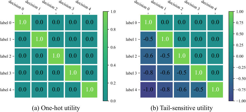
We first discuss the design of the utility function: $u(y,d)$, where $y$ is the ground truth (true label) and $d$ is the decision (predicted label). The utility function defines the gain of making different decisions and can encode our preference for specific metrics in various tasks. The utility function is a standard component in Decision Theory and its design has been comprehensively studied in the literature. For example, Chapter 2.2 of Robert et al. 2007 guarantees the existence of utility functions with rational decision-makers. Generally, the values of the utility function over all class labels are stored in a form of utility matrix $\bm{U}$, where $U_{ij}=u(y=i,d=j)$.

In a standard classification setting, the overall accuracy is the most decisive metric in evaluation. It only matters whether the decision is consistent with the ground truth (i.e., $y=d$). Therefore, as shown in Fig. 1(a), a simple one-hot utility can be defined by $u(y,d)=\mathbbm{1}\{y=d\}$, which is corresponding to the standard accuracy metric.

In modern applications of long-tailed classification, the semantic importance of “tailed” data often implies more penalty in the circumstance of predicting tailed samples as head (Sengupta et al. 2016; Rahman et al. 2021; Yang et al. 2022). Besides, the lack of training samples in tailed classes has been empirically proved to be the bottleneck of classification performance (Li et al. 2022). Therefore, the ratio of false head samples in evaluation would reflect the potential of a model in real-world applications ²² 2 The quantitative form will be discussed in Section 6.3.. To this end, a tail-sensitive utility can be defined by adding an extra penalty on those false head samples, as shown in Fig. 1(b). The tail-sensitive utility encourages the model to predict any uncertain sample as tail rather than head, while not affecting the predictions of the true class when the model is confident.

Due to the discrepancy between training (long-tailed) and testing (uniform) data distributions, we propose to compute the integrated gain with the posterior of testing data $p(\bm{\theta}|\mathcal{D}_{test})$ to target at evaluation, where $\mathcal{D}_{test}=\{(\bm{x}_{i},y_{i})\}_{i=1}^{N}$ with $(\bm{x}_{i},y_{i})\sim p_{test}(\bm{x},y)$. To infer the posterior $p(\bm{\theta}|\mathcal{D}_{test})$, we use the variational method where a variational distribution $q(\bm{\theta})$ is introduced to the lower bound of the integrated gain in Eq. 5:

where $(\bm{x}_{i},y_{i})$ is training data but we forcefully compute its probability on testing distribution, and $C$ is a constant. Eq. 6 is proved in Appendix C and the main idea is to apply Jensen’s inequality (Jensen 1906). The lower bound $L(q,d)$ is our training objective and it provides a cross-entropy-like way to update the variational distribution $q(\bm{\theta})$, and most importantly, converts the data distribution from $p_{test}(\bm{x},y)$ (uniform) to $p_{train}(\bm{x},y)$ (long-tailed) by the technique of importance sampling (Kloek & Van Dijk 1978) to make the computation during training possible³³ 3 Thanks to the fact that training and testing data are semantically identical..

Moreover, the variational distribution $q(\bm{\theta})$ is guaranteed to be an approximation of the posterior $p(\bm{\theta}|\mathcal{D}_{test})$, because Eq. 6 contains Bayesian inference on the posterior of testing data. To support this, we look into the KL divergence between $q(\bm{\theta})$ and $p(\bm{\theta}|\mathcal{D}_{test})$:

where $C$ is a constant. Eq. 7 is proved in Appendix D. Comparing Eq. 6 and Eq. 7, it is clear that part of the objective at inference step is Bayesian inference on the posterior of testing data, with $q(\bm{\theta})$ approaching $p(\bm{\theta}|\mathcal{D}_{test})$.⁴⁴ 4 In fact, $q(\bm{\theta})$ approximates the gain-calibrated posterior: $\tilde{p}(\bm{\theta}|\mathcal{D}_{test})\propto p(\bm{\theta}|\mathcal{D}_{test})\prod_{y^{\prime}}p(y^{\prime}|\bm{x}_{i},\bm{\theta})^{u(y^{\prime},d(\bm{x}_{i}))}$.

In summary, the objective $L(q,d)$ in Eq. 6 enables the framework to simultaneously consider inference, decision (utility), and data distribution ($p_{test}(\bm{x},y)/p_{train}(\bm{x},y)$, which will be further discussed in Section 5.1). It provides a principled way to optimize the integrated gain in Eq. 5.

To optimize $L(q,d)$ w.r.t the decision $d$, one way is to select the decision $d^{\star}$ that maximizes the gain respectively for each input $\bm{x}_{i}$ given the current variational distribution:

Notably, for symmetric utility functions (e.g., one-hot utility), Eq. 8 can be further simplified: $d^{\star}=\argmax_{d}\mathbb{E}_{\bm{\theta}\sim q(\bm{\theta})}\log{p(d|\bm{x},\bm{\theta})}$, which is equivalent to the maximum of the predictive distribution.

However, during training, we essentially know that the optimal decisions for training data are their true labels. Therefore, we can utilize this knowledge and simply set $d(x_{i})=y_{i}$. We can also view this as selecting the optimal decisions under a well-estimated $q(\bm{\theta})$ in Eq. 8 instead of the current distribution, since we expect $d^{\star}$ approach the true labels as $q(\bm{\theta})$ keeps updating. Then the objective can be further simplified to be:

During testing, we use Eq. 8 to select the decision for testing data $\bm{x}_{i}$.

At the inference step, we exploit the importance sampling to convert $p(\mathcal{D}_{test})$ to $p(\mathcal{D}_{train})$ and obtain a discrepancy ratio $p_{test}(\bm{x},y)/p_{train}(\bm{x},y)$. Recall that in long-tailed distribution, the training and testing data are semantically identical, and thus the model prediction must be the same for an input regardless of being in the training or testing set (i.e., $p_{train}(y|\bm{x},\bm{\theta})=p_{test}(y|\bm{x},\bm{\theta})$). Therefore, the discrepancy ratio can be further simplified by:

which only depends on the class probabilities of training and testing data. Since we assume a uniform distribution for the testing set in long-tailed data, the probability $p_{test}(\bm{y})$ would be a constant for all $\bm{x}$, and thus the discrepancy ratio is equivalent to:

where $f$ is an increasing function and $n_{y}$ refers to the number of samples in the class $y$. We introduce the notation of $f(n_{y})$ because the class probability only depend on the number of samples in this class.

The choices of $f$ can determine different strategies used by previous re-balancing methods in long-tailed classification. For example, $f(n_{y})=n_{y}^{\gamma}$ is the most conventional choice with a sensitivity factor $\gamma$ to control the importance of head classes (Huang et al. 2016; Wang et al. 2017; Pan et al. 2021); $f(n_{y})=(1-\beta^{n_{y}})/(1-\beta)$ is the effective number which considers data overlap (Cui et al. 2019). A detailed analysis on the choice of discrepancy ratios will be conducted in Section 6.5. Notably, our framework is compatible with all previous re-balancing methods as long as they can be expressed in the form of $1/f(n_{y})$.

To pursue the efficiency of model architecture, we use particle optimization (Liu & Wang 2016; D’Angelo & Fortuin 2021) to obtain the variational distribution: $q(\bm{\theta})=\sum_{j=1}^{M}w_{j}\cdot\delta(\bm{\theta}-\bm{\theta}_{j})$, where $\{w_{j}\}_{j=1}^{M}$ are normalized weights which hold $\sum_{j=1}^{M}w_{j}=1$, and $\delta(\cdot)$ is the Dirac delta function. The “particles” $\{\bm{\theta}_{j}\}_{j=1}^{M}$ are implemented by ensemble model, which has been empirically explored on the long-tailed data (Wang et al. 2020; Li et al. 2022). Our formulation gives theoretical justification to ensemble approaches in long-tailed problems: Due to the scarcity of tailed data, there is not enough evidence to support a single solution, leading to many equally good solutions (which give complementary predictions) in the loss landscape. Thus, estimating the full posterior is essential to provide a comprehensive characterization of the solution space. Particle optimization reduces the cost of Bayesian inference and is more efficient than variational inference and Markov chain Monte Carlo (MCMC), especially on high-dimensional and multimodal distributions. Besides, the computational cost of our method can be further reduced by leveraging recent techniques, such as partially being Bayesian in model architectures (Kristiadi et al. 2020).

In Eq. 6, the regularization term $KL(q(\bm{\theta})||p(\bm{\theta}))$ guarantees the variational distribution to approach the posterior as training proceeds. If we assume the prior $p(\bm{\theta})$ to be Gaussian, the regularization can be extended to:

where $\lambda$ is a constant, $\Theta$ is the parameter space, and $H(\bm{\theta})$ is the entropy of $\bm{\theta}$. The $L_{2}$-regularization prevents the model from over-fitting and the entropy term applies a repulsive force to the particles to promote their diversity, pushing the particles to the target posterior (D’Angelo & Fortuin 2021). A simple approximation for the entropy is used in this paper:

where $\hat{\Sigma}_{\bm{\theta}}$ is the covariance matrix estimated by those particles. Other entropy approximations can also be used. By the technique of SWAG-diagonal covariance (Maddox et al. 2019), the covariance matrix can then be directly computed by: $\hat{\Sigma}_{\bm{\theta}}=diag(\overline{\bm{\theta}^{2}}-\overline{\bm{\theta}}^{2})$.

Overall, the regularization term is a combination of $L_{2}$ weight decay and repulsive force, and is computed by:

Our regularization is different from existing diversity regularization (Wang et al. 2020), and is more principled and naturally derived from the integrated gain.

In summary, our method, with principled design and theoretical justification, is essentially cheap and easy to implement and can be used as a drop-in replacement for existing re-balancing and ensemble methods in general long-tailed problems. We outline our algorithm in Appendix B.

Classification accuracy is the most standard benchmark for long-tailed data, where the overall accuracy and accuracies for three class regions are evaluated. Classes are equally split into three class regions (head, med and tail). For example, there are 33, 33 and 34 classes respectively in the head, med and tail regions of CIFAR-100-LT. The classification results are shown in Table 1 and Table 2. We apply the one-hot utility in our method to accord with standard accuracy metric. Our method consistently outperforms all other compared methods in terms of overall accuracy. For regional accuracies, our method achieves the best performances on all class regions in most cases. In particular, our method significantly outperforms previous methods on the crucial tailed data, while being comparable or even better on med and head classes. These results demonstrate the effectiveness of taking a Bayesian-decision-theory perspective on the long-tailed problem.

As discussed previously, classifying tailed samples into head classes would often induce negative consequences in real-world applications. Therefore, we are interested in quantifying how likely it will happen, and further evaluating the tail sensitivity of the compared methods. Inspired by the false positive rate, we define the False Head Rate (FHR) as:

where $TH$ is the number of samples that are labeled as tail but predicted as head, and $TT$ is the number of samples that are labeled and predicted as tail. We also consider different settings of tail region, and select the last 25%, 50% and 75% classes as tail. We apply the tail-sensitive utility in Fig. 1(b) to our method. From Table 3, we observe significant improvements of LBD over previous methods under all settings, especially on the relatively small CIFAR datasets, which means that the “false head risk” is more severe on smaller datasets with scarce tailed samples. This shows the importance of taking the decision loss into account and also demonstrates the flexibility of our framework which is compatible with different utilities, leading to better performance for different types of tasks. In contrast, previous methods do not coonsider decision loss and may result in undesirable consequences when some type of errors have high costs.

In our method, the predictive uncertainty can be naturally obtained by the entropy of predictive distribution (Malinin & Gales 2018). For the compared uncertainty algorithms, MCP is a trivial baseline which obtains uncertainty scores from the maximum value of softmax distribution, which is added to the RIDE (Wang et al. 2020) backbone; evidential uncertainty is rooted in the subjective logic (Audun 2018), and is introduced to long-tailed classification by TLC (Li et al. 2022). We evaluate the uncertainty algorithms with AUC (McClish 1989) and ECE (Naeini et al. 2015), which are shown in Table 4. Our Bayesian predictive uncertainty outperforms the other two counterparts and has a remarkable advantage on the ECE metric, demonstrating the superiority of using principled Bayesian uncertainty quantification.

References

- Audun (2018) Audun, J. Subjective Logic: A formalism for reasoning under uncertainty. Springer, 2018.
- Berger (1985) Berger, J. O. Statistical decision theory and Bayesian analysis. Springer Science & Business Media, 1985.
- Bottou (1998) Bottou, L. Online algorithms and stochastic approxima-p tions. Online learning and neural networks, 1998.
- Cao et al. (2019) Cao, K., Wei, C., Gaidon, A., Arechiga, N., and Ma, T. Learning imbalanced datasets with label-distribution-aware margin loss. Advances in neural information processing systems, 32, 2019.
- Chen et al. (2018) Chen, C., Zhang, R., Wang, W., Li, B., and Chen, L. A unified particle-optimization framework for scalable bayesian sampling. stat, 1050:10, 2018.
- Chu et al. (2020) Chu, P., Bian, X., Liu, S., and Ling, H. Feature space augmentation for long-tailed data. In Computer Vision–ECCV 2020: 16th European Conference, Glasgow, UK, August 23–28, 2020, Proceedings, Part XXIX 16, pp. 694–710. Springer, 2020.
- Cobb et al. (2018) Cobb, A. D., Roberts, S. J., and Gal, Y. Loss-calibrated approximate inference in bayesian neural networks. arXiv preprint arXiv:1805.03901, 2018.
- Cui et al. (2019) Cui, Y., Jia, M., Lin, T.-Y., Song, Y., and Belongie, S. Class-balanced loss based on effective number of samples. In Proceedings of the IEEE/CVF conference on computer vision and pattern recognition, pp. 9268–9277, 2019.
- D’Angelo & Fortuin (2020) D’Angelo, F. and Fortuin, V. Annealed stein variational gradient descent. In Third Symposium on Advances in Approximate Bayesian Inference, 2020.
- D’Angelo & Fortuin (2021) D’Angelo, F. and Fortuin, V. Repulsive deep ensembles are bayesian. Advances in Neural Information Processing Systems, 34:3451–3465, 2021.
- Dempster et al. (1977) Dempster, A. P., Laird, N. M., and Rubin, D. B. Maximum likelihood from incomplete data via the em algorithm. Journal of the Royal Statistical Society: Series B (Methodological), 39(1):1–22, 1977.
- Deng et al. (2009) Deng, J., Dong, W., Socher, R., Li, L.-J., Li, K., and Fei-Fei, L. Imagenet: A large-scale hierarchical image database. In 2009 IEEE conference on computer vision and pattern recognition, pp. 248–255. Ieee, 2009.
- Dietterich (2000) Dietterich, T. G. Ensemble methods in machine learning. In International workshop on multiple classifier systems, pp. 1–15. Springer, 2000.
- Ganaie et al. (2021) Ganaie, M. A., Hu, M., et al. Ensemble deep learning: A review. arXiv preprint arXiv:2104.02395, 2021.
- Geng et al. (2020) Geng, C., Huang, S.-j., and Chen, S. Recent advances in open set recognition: A survey. IEEE transactions on pattern analysis and machine intelligence, 43(10):3614–3631, 2020.
- Han et al. (2005) Han, H., Wang, W.-Y., and Mao, B.-H. Borderline-smote: a new over-sampling method in imbalanced data sets learning. In International conference on intelligent computing, pp. 878–887. Springer, 2005.
- Hand (2006) Hand, D. J. Classifier technology and the illusion of progress. Statistical science, 21(1):1–14, 2006.
- Hendrycks & Gimpel (2017) Hendrycks, D. and Gimpel, K. A baseline for detecting misclassified and out-of-distribution examples in neural networks. Proceedings of International Conference on Learning Representations, 2017.
- Huang et al. (2016) Huang, C., Li, Y., Loy, C. C., and Tang, X. Learning deep representation for imbalanced classification. In Proceedings of the IEEE conference on computer vision and pattern recognition, pp. 5375–5384, 2016.
- Jensen (1906) Jensen, J. L. W. V. Sur les fonctions convexes et les inégalités entre les valeurs moyennes. Acta mathematica, 30(1):175–193, 1906.
- Kim et al. (2020) Kim, J., Jeong, J., and Shin, J. M2m: Imbalanced classification via major-to-minor translation. In Proceedings of the IEEE/CVF Conference on Computer Vision and Pattern Recognition, pp. 13896–13905, 2020.
- Kloek & Van Dijk (1978) Kloek, T. and Van Dijk, H. K. Bayesian estimates of equation system parameters: an application of integration by monte carlo. Econometrica: Journal of the Econometric Society, pp. 1–19, 1978.
- Korba et al. (2020) Korba, A., Salim, A., Arbel, M., Luise, G., and Gretton, A. A non-asymptotic analysis for stein variational gradient descent. Advances in Neural Information Processing Systems, 33:4672–4682, 2020.
- Krishna et al. (2017) Krishna, R., Zhu, Y., Groth, O., Johnson, J., Hata, K., Kravitz, J., Chen, S., Kalantidis, Y., Li, L.-J., Shamma, D. A., et al. Visual genome: Connecting language and vision using crowdsourced dense image annotations. International journal of computer vision, 123(1):32–73, 2017.
- Kristiadi et al. (2020) Kristiadi, A., Hein, M., and Hennig, P. Being bayesian, even just a bit, fixes overconfidence in relu networks. In International conference on machine learning, pp. 5436–5446. PMLR, 2020.
- Krizhevsky & Hinton (2009) Krizhevsky, A. and Hinton, G. Learning multiple layers of features from tiny images. Technical Report 0, University of Toronto, Toronto, Ontario, 2009.
- Lacoste-Julien et al. (2011) Lacoste-Julien, S., Huszár, F., and Ghahramani, Z. Approximate inference for the loss-calibrated bayesian. In Proceedings of the Fourteenth International Conference on Artificial Intelligence and Statistics, pp. 416–424. JMLR Workshop and Conference Proceedings, 2011.
- Lakshminarayanan et al. (2017) Lakshminarayanan, B., Pritzel, A., and Blundell, C. Simple and scalable predictive uncertainty estimation using deep ensembles. Advances in Neural Information Processing Systems, 30, 2017.
- Li et al. (2022) Li, B., Han, Z., Li, H., Fu, H., and Zhang, C. Trustworthy long-tailed classification. In Proceedings of the IEEE/CVF Conference on Computer Vision and Pattern Recognition, pp. 6970–6979, 2022.
- Lin et al. (2014) Lin, T.-Y., Maire, M., Belongie, S., Hays, J., Perona, P., Ramanan, D., Dollár, P., and Zitnick, C. L. Microsoft coco: Common objects in context. In European conference on computer vision, pp. 740–755. Springer, 2014.
- Lin et al. (2017) Lin, T.-Y., Goyal, P., Girshick, R., He, K., and Dollár, P. Focal loss for dense object detection. In Proceedings of the IEEE international conference on computer vision, pp. 2980–2988, 2017.
- Liu et al. (2018) Liu, C., Zhuo, J., Cheng, P., Zhang, R., Zhu, J., and Carin, L. Accelerated first-order methods on the wasserstein space for bayesian inference. stat, 1050:4, 2018.
- Liu et al. (2019a) Liu, C., Zhuo, J., Cheng, P., Zhang, R., and Zhu, J. Understanding and accelerating particle-based variational inference. In International Conference on Machine Learning, pp. 4082–4092. PMLR, 2019a.
- Liu et al. (2020) Liu, J., Sun, Y., Han, C., Dou, Z., and Li, W. Deep representation learning on long-tailed data: A learnable embedding augmentation perspective. In Proceedings of the IEEE/CVF Conference on Computer Vision and Pattern Recognition, pp. 2970–2979, 2020.
- Liu (2017) Liu, Q. Stein variational gradient descent as gradient flow. Advances in neural information processing systems, 30, 2017.
- Liu & Wang (2016) Liu, Q. and Wang, D. Stein variational gradient descent: A general purpose bayesian inference algorithm. Advances in neural information processing systems, 29, 2016.
- Liu et al. (2008) Liu, X.-Y., Wu, J., and Zhou, Z.-H. Exploratory undersampling for class-imbalance learning. IEEE Transactions on Systems, Man, and Cybernetics, Part B (Cybernetics), 39(2):539–550, 2008.
- Liu et al. (2019b) Liu, Z., Miao, Z., Zhan, X., Wang, J., Gong, B., and Yu, S. X. Large-scale long-tailed recognition in an open world. In Proceedings of the IEEE/CVF Conference on Computer Vision and Pattern Recognition, pp. 2537–2546, 2019b.
- Maddox et al. (2019) Maddox, W. J., Izmailov, P., Garipov, T., Vetrov, D. P., and Wilson, A. G. A simple baseline for bayesian uncertainty in deep learning. Advances in Neural Information Processing Systems, 32, 2019.
- Mahajan et al. (2018) Mahajan, D., Girshick, R., Ramanathan, V., He, K., Paluri, M., Li, Y., Bharambe, A., and Van Der Maaten, L. Exploring the limits of weakly supervised pretraining. In Proceedings of the European conference on computer vision (ECCV), pp. 181–196, 2018.
- Malinin & Gales (2018) Malinin, A. and Gales, M. Predictive uncertainty estimation via prior networks. Advances in neural information processing systems, 31, 2018.
- McClish (1989) McClish, D. K. Analyzing a portion of the roc curve. Medical decision making, 9(3):190–195, 1989.
- Menon et al. (2020) Menon, A. K., Jayasumana, S., Rawat, A. S., Jain, H., Veit, A., and Kumar, S. Long-tail learning via logit adjustment. In International Conference on Learning Representations, 2020.
- Morais & Pillow (2022) Morais, M. J. and Pillow, J. W. Loss-calibrated expectation propagation for approximate bayesian decision-making. arXiv preprint arXiv:2201.03128, 2022.
- Moreno-Torres et al. (2012) Moreno-Torres, J. G., Raeder, T., Alaiz-Rodríguez, R., Chawla, N. V., and Herrera, F. A unifying view on dataset shift in classification. Pattern recognition, 45(1):521–530, 2012.
- Naeini et al. (2015) Naeini, M. P., Cooper, G., and Hauskrecht, M. Obtaining well calibrated probabilities using bayesian binning. In Twenty-Ninth AAAI Conference on Artificial Intelligence, 2015.
- Nam et al. (2023) Nam, G., Jang, S., and Lee, J. Decoupled training for long-tailed classification with stochastic representations. In The Eleventh International Conference on Learning Representations, 2023.
- Pan et al. (2021) Pan, T.-Y., Zhang, C., Li, Y., Hu, H., Xuan, D., Changpinyo, S., Gong, B., and Chao, W.-L. On model calibration for long-tailed object detection and instance segmentation. Advances in Neural Information Processing Systems, 34:2529–2542, 2021.
- Quinonero-Candela et al. (2008) Quinonero-Candela, J., Sugiyama, M., Schwaighofer, A., and Lawrence, N. D. Dataset shift in machine learning. Mit Press, 2008.
- Rahman et al. (2021) Rahman, A., Hassan, I., and Ahad, M. A. R. Nurse care activity recognition: A cost-sensitive ensemble approach to handle imbalanced class problem in the wild. In Adjunct Proceedings of the 2021 ACM International Joint Conference on Pervasive and Ubiquitous Computing and Proceedings of the 2021 ACM International Symposium on Wearable Computers, pp. 440–445, 2021.
- Reed (2001) Reed, W. J. The pareto, zipf and other power laws. Economics letters, 74(1):15–19, 2001.
- Robert et al. (2007) Robert, C. P. et al. The Bayesian choice: from decision-theoretic foundations to computational implementation, volume 2. Springer, 2007.
- Schervish (2012) Schervish, M. J. Theory of statistics. Springer Science & Business Media, 2012.
- Sengupta et al. (2016) Sengupta, S., Chen, J.-C., Castillo, C., Patel, V. M., Chellappa, R., and Jacobs, D. W. Frontal to profile face verification in the wild. In 2016 IEEE winter conference on applications of computer vision (WACV), pp. 1–9. IEEE, 2016.
- Şensoy et al. (2018) Şensoy, M., Kaplan, L., and Kandemir, M. Evidential deep learning to quantify classification uncertainty. Advances in Neural Information Processing Systems, 2018.
- Vadera et al. (2021) Vadera, M. P., Ghosh, S., Ng, K., and Marlin, B. M. Post-hoc loss-calibration for bayesian neural networks. In Uncertainty in Artificial Intelligence, pp. 1403–1412. PMLR, 2021.
- Van Horn & Perona (2017) Van Horn, G. and Perona, P. The devil is in the tails: Fine-grained classification in the wild. arXiv preprint arXiv:1709.01450, 2017.
- Wang et al. (2022) Wang, H., Zhang, A., Zhu, Y., Zheng, S., Li, M., Smola, A. J., and Wang, Z. Partial and asymmetric contrastive learning for out-of-distribution detection in long-tailed recognition. In International Conference on Machine Learning, pp. 23446–23458. PMLR, 2022.
- Wang et al. (2020) Wang, X., Lian, L., Miao, Z., Liu, Z., and Yu, S. Long-tailed recognition by routing diverse distribution-aware experts. In International Conference on Learning Representations, 2020.
- Wang et al. (2017) Wang, Y.-X., Ramanan, D., and Hebert, M. Learning to model the tail. Advances in neural information processing systems, 30, 2017.
- Wang et al. (2018) Wang, Z., Ren, T., Zhu, J., and Zhang, B. Function space particle optimization for bayesian neural networks. In International Conference on Learning Representations, 2018.
- Wu et al. (2020) Wu, T., Huang, Q., Liu, Z., Wang, Y., and Lin, D. Distribution-balanced loss for multi-label classification in long-tailed datasets. In European Conference on Computer Vision, pp. 162–178. Springer, 2020.
- Xiang et al. (2020) Xiang, L., Ding, G., and Han, J. Learning from multiple experts: Self-paced knowledge distillation for long-tailed classification. In European Conference on Computer Vision, pp. 247–263. Springer, 2020.
- Yang et al. (2022) Yang, Z., Pan, J., Yang, Y., Shi, X., Zhou, H.-Y., Zhang, Z., and Bian, C. Proco: Prototype-aware contrastive learning for long-tailed medical image classification. In International Conference on Medical Image Computing and Computer-Assisted Intervention, pp. 173–182. Springer, 2022.
- Zhang et al. (2022) Zhang, Y., Hooi, B., Lanqing, H., and Feng, J. Self-supervised aggregation of diverse experts for test-agnostic long-tailed recognition. In Advances in Neural Information Processing Systems, 2022.
Appendix A Decision Gain
As mentioned in the paper, we design the decision gain to be the following: