Automated Crack Propagation Measurement On Asphalt Concrete Specimens Using an Optical Flow-Based Deep Neural Network
Abstract
This article proposes a deep neural network, namely CrackPropNet, to measure crack propagation on asphalt concrete (AC) specimens. It offers an accurate, flexible, efficient, and low-cost solution for crack propagation measurement using images collected during cracking tests. CrackPropNet significantly differs from traditional deep learning networks, as it involves learning to locate displacement field discontinuities by matching features at various locations in the reference and deformed images. An image library representing the diversified cracking behavior of AC was developed for supervised training. CrackPropNet achieved an optimal dataset scale F-1 of 0.755 and optimal image scale F-1 of 0.781 on the testing dataset at a running speed of 26 frame-per-second. Experiments demonstrated that low to medium-level Gaussian noises had a limited impact on the measurement accuracy of CrackPropNet. Moreover, the model showed promising generalization on fundamentally different images. As a crack measurement technique, the CrackPropNet can detect complex crack patterns accurately and efficiently in AC cracking tests. It can be applied to characterize the cracking phenomenon, evaluate AC cracking potential, validate test protocols, and verify theoretical models.
keywords
Asphalt Concrete, crack propagation, digital image correlation, optical flow, deep learning.1 Introduction
Approximately 95 percent of paved roads in the United States are surfaced with asphalt. Cracking is a common mode of failure in asphalt concrete (AC) pavements. Many tests have been developed to assess the cracking potential of AC materials. Accurate monitoring of crack initiation and propagation during testing is crucial.
Contact tools like a linear variable differential transformer (LVDT), extensometers, strain gauges, and crack mouth opening displacement (CMOD) clip gauges are the most widely used methods to monitor crack propagation and opening in AC cracking tests. However, these tools only provide localized information, as the measurement location must be decided before testing. As shown in Figure 1, the CMOD clip gauge is attached at the bottom of the specimen when conducting the low-temperature semi-circular bending (SCB) test (Li & Marasteanu (2010)). As such, the crack opening is only recorded at that location. Similarly, the above-mentioned contact techniques may only provide indirect crack propagation and opening measurements. For example, the load-line displacement (LLD), measured by an extensometer mounted vertically at the surface of the specimen, is used to estimate crack propagation speed. However, a such approximation is insufficient to describe the cracking phenomenon, as a crack tends to choose a path around the aggregate as it grows (Doll et al. (2017)). In addition, orienting the contact devices is time-consuming and requires experience, especially on small specimens. Moreover, routine calibrations are needed to ensure accurate measurement. Therefore, developing an easy-to-use, accurate, and full-field crack measurement technique for AC cracking tests is imperative.

Low-level computer vision-based crack detection methods have been proposed. The most popular algorithms include thresholding, image segmentation, filtering, and blob extraction (Hartman & Gilchrist (2004); Oliveira & Correia (2009); Ying & Salari (2010); A. Zhang et al. (2013); Wang et al. (2018)). However, the limitation of these methods is obtaining accurate results under complex imaging environments. Deep learning, especially deep convolution neural network (CNN), has been widely used to detect and categorize cracks (Cha et al. (2017); L. Zhang et al. (2016); A. Zhang et al. (2017); Fei et al. (2019)). However, these models were mainly developed for visible mature cracks; the ground truth verification relied on visual recognition. This renders the models mentioned above unsuitable for monitoring crack propagation in AC cracking tests, where small cracks in the early stages are critical but often difficult to visualize.
The digital image correlation (DIC) technique has the potential to overcome these challenges. The DIC is an optical method that measures full-field displacement and strain. Because surface cracks are defined as displacement field discontinuities, cracks with varying sizes could be located, given an accurate displacement field. A few attempts have been made to measure cracks using DIC. Due to complex crack growth, locating cracks based on DIC-measured displacement or strain field is a challenge. Current methods rely on the strain or displacement thresholding, which requires significant post-processing efforts and empirical knowledge (Buttlar et al. (2014); Safavizadeh & Kim (2017)). In addition, DIC analysis involves computationally expensive optimization, making it unsuitable for real-time applications such as crack propagation measurement in AC testing, where hundreds or thousands of images need to be analyzed. These limitations have limited the implementation of DIC as an automated crack measurement technique for AC cracking tests.
This article proposes a deep neural network to automatically measure crack propagation during testing based on the optical flow concept. Compared to the existing techniques discussed above, it offers an accurate, flexible, efficient, and low-cost solution. It can accurately measure crack propagation from hundreds of images collected by low-cost cameras in less than one minute.
This paper has seven sections, and they are organized as the following: section one discusses the background and motivation of this study; section two presents the development of the database; section three introduces the architecture of the deep neural network; section four explains the training strategy; section five presents the evaluation of the proposed network; section six discusses advantages and possible applications of the CrackPropNet, and the conclusions and recommendations are presented in section seven.
2 Data Preparation
As shown in Figure 2, the data preparation process consists of four steps:
- 1.
Collect raw images;
- 2.
Compute displacement fields using DIC;
- 3.
Label ground-truth crack edges;
- 4.
Inspect and verify ground-truth labels.
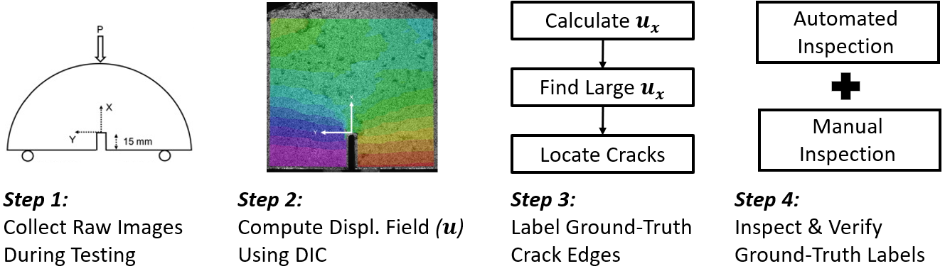
Implementation details are described in the following sections.
2.1 Raw Image Collection
Raw images were collected while conducting the Illinois Flexibility Index Test (I-FIT), as shown in Figure 4 (Ozer, Al-Qadi, Lambros et al. (2016); Ozer, Al-Qadi, Singhvi et al. (2016)). An extensive testing program covering a wide range of testing conditions and materials was developed. The goal was to develop an extensive image database covering AC’s diversified cracking behavior. All experiments were displacement controlled. Load-line displacement was used on room-temperature tests, while CMOD was used under low temperatures to provide better crack propagation stability (Doll et al. (2017)). Two different testing temperatures: -12 and 25°C; and four different loading rates: 0.7, 6.25, 25, and 50 mm/min were considered. The fracture behavior of AC is time- and temperature-dependent. A more brittle failure is expected at lower temperatures or higher loading rates (Al-Qadi et al. (2015)). As shown in Figure 3, a total of 53 AC mixes were tested. They had different N-designs, binder types and content, aggregate mineralogy, and the amount of recycled materials. The I-FIT specimens were prepared either from lab-compacted cylindrical pills or field cores. All specimens had SCB geometry, as shown in Figure 1, while their thickness, notch length, and air void range from 25mm to 60mm, 10mm to 35mm, and 1% to 12%, respectively. For each I-FIT specimen, a speckle pattern consisting of a white layer of paint and a random black pattern on top was applied (Doll et al. (2017)).

Two CCD (Charge Coupled Device) cameras were positioned perpendicularly to the surface of the I-FIT specimen to collect images during the test: a Point Grey Gazelle 4.1MP Mono ( pixels, 150 frames per second-fps) and an Allied Vision Prosilica GX6600 ( pixels, 4 fps) with a Tokina AT-X Pro Macro 100 2.8D lens. The Gazelle has a faster acquisition rate but a lower resolution than the Prosilica. The former is generally used in experiments where the materials can be considered homogeneous, while the latter aims to study damage zone evolution in heterogeneous materials such as AC. The database intentionally includes images taken from cameras with significantly different resolutions to ensure better generalization of the deep neural network.

2.2 Compute Displacement Fields Using DIC
The displacement fields were first computed using DIC. The DIC works by tracking pixels in a sequence of images. This is achieved using area-based matching, which extracts gray value correspondences based on their similarities. First, a reference image was taken at the unloaded state, and an area of interest was selected. Then, a subset of pixels is compared to a deformed image taken at a loaded state to identify the best match. Finally, the deformation of a point in the subset can be computed using Equation 1, which allows for translation, rotation, shear, and combinations.

| (1) |
As shown in Figure 5, and are Cartesian coordinates of a point in the reference image; and refer to its coordinates in the deformed image; and denote the corresponding displacement components of the reference subset center in the x- and y- direction, respectively; , , , are the first-order displacement gradients of the reference subset; and . To provide adequate spatial resolution to resolve the displacement distribution between and within aggregate particles, the subset size used for correlation was carefully chosen for each test following the algorithm proposed by Pan et al. (2008).
2.3 Ground-Truth Crack Edges Labeling
Once the displacement field was obtained, potential crack edges could be located following the method proposed by Zhu & Al-Qadi (2023). Figure 6 shows the displacement field () contour plot measured by DIC for an I-FIT specimen surface, where a crack is visible in the area of interest. The reference and deformed images were taken with the Gazelle camera when conducting the I-FIT test at 25°C with a 50mm/min loading rate. A subset size of with a correlation point spacing of 11 pixels was used for DIC analysis. This resulted in a spatial resolution of approximately 25 and produced roughly square microns in the area of interest.

Then, the first-order derivative of the opening displacement was obtained by filtering the displacement field with a kernel. For example, Figure 7 plots along three discrete axes ( , , and ). A large indicates the material separation between the two correlation points, suggesting a crack may present. Thus, potential crack edges could be found by locating the corresponding correlation points in the deformed image, as shown in Figure 8. Please note that the marked crack edges may not match the actual crack edges exactly because the correlation point spacing is usually larger than 1 pixel in DIC analysis. However, the effect is negligible as the spatial resolution is typically smaller than 25 , which results in an error of less than 0.3 mm. In this article, the target value for a crack edge pixel is 1, while the rest is 0.


2.4 Verification of Ground-Truth Labels
The above-described procedure may falsely label some pixels as crack edges under certain circumstances. For example, suppose an I-FIT specimen has irregularities and holes on the surface that cannot be painted or create shadows. In that case, the error in DIC measurements will increase compared to experiments on flat surfaces. This may lead to falsely labeled crack edge pixels. To make the ground-truth crack edges as accurate as possible, every image went through two rounds of inspection:
- 1.
Automated inspection: for a sequence of deformed images, if pixel was labeled as a crack edge in frame , but not in the following frames , the label would be corrected. In contrast, if pixel was not labeled as crack edge in frame , but was labeled in previous and following frames , the label would be corrected;
- 2.
Manual inspection: the ground-truths were visually inspected and verified.
2.5 Image Library Summary
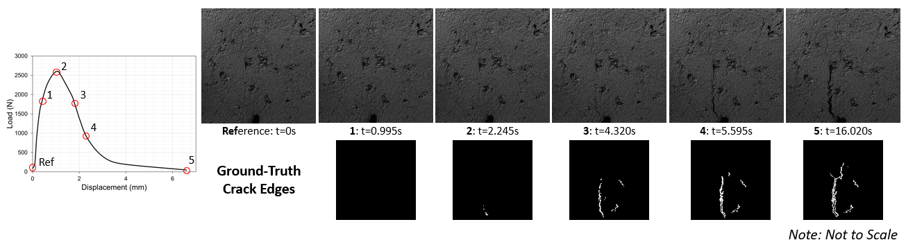
An image library, made of pairs of images with and crack edge labels, was developed for supervised learning. It consisted of 2,560 frame pairs. The image library represented the diversified cracking behavior of AC. Images were collected in the past eight years by four different operators. The original images collected by the Gazelle and the Prosilica camera have resolutions of and , respectively. The original image was downsized to by min-pooling and cropping to balance computational overhead and accuracy. This resulted in a spatial resolution of approximately 0.05 mm/pixel. Because the correlation point spacing in DIC analysis was typically larger than 10 pixels, the labeled ground truth crack edges were discontinuous. To provide more accurate ground-truth labels and reduce the computational cost, the ground-truth crack edge map was downsized from the original resolution to . This resulted in a spatial resolution of approximately 0.4 mm/pixel, which is adequate in this task, where the measurement area is larger than . Figure 9 illustrates a sequence of images together with their ground-truth crack edge maps. They were collected while conducting an I-FIT test on a typical AC mix (an Illinois N90 mix) at 25 mm/min and 25°C.
To evaluate the sufficiency of the developed image library, Table 2.5 compared it with datasets used in previous studies for relative tasks. The size of the developed image library is comparable to existing datasets. It is worth noting that StrainNet uses synthetic images, which have the advantage of developing large datasets quickly and inexpensively. However, real images were used in this paper because of the complexity of crack shapes in AC testing.
Comparison with datasets used in previous studies for relative tasks. Dataset Number of frames Resolution Type Task: Pavement crack detection CRACK500 (Yang et al. (2019)) 500 20001500 Real GAPs384 (Eisenbach et al. (2017)) 1,969 19201080 Real CrackNet (A. Zhang et al. (2017)) 2,000 1024512 Real CrackNet-V (Fei et al. (2019)) 3,083 1024512 Real Task: Optical flow estimation KITTI2015 (Menze & Geiger (2015)) 800 pairs 1242375 Real Sintel (Butler et al. (2012)) 1064 pairs 960540 Real Task: DIC with deep learning StrainNet (Boukhtache et al. (2021)) 363 reference frames 256256 Synthetic Proposed 2,560 pairs 10241024 Real
3 Network Architecture
Training a deep CNN from scratch requires a large dataset and significant computational power, which is impossible in most situations. In practice, pre-trained networks could be used as initialization or feature extractors for the task of interest. Because surface cracks are defined as displacement field discontinuities, crack propagation measurement in AC fracture testing can be accomplished by stacking edge detection layers on pre-trained networks for optical flow estimation.
This section provides a brief overview of existing networks on optical flow estimation. The proposed network architecture is discussed in detail.
3.1 CNN-Based Methods for Optical Flow Estimation
Optical flow is the pattern of apparent motion of objects due to the relative motion between an observer and a visual scene (Warren & Strelow (2013)). Traditional energy-minimization-based approaches involve computationally expensive optimization, making them unsuitable for large-scale real-time applications such as crack propagation measurement in AC testing, where hundreds of images need to be processed.
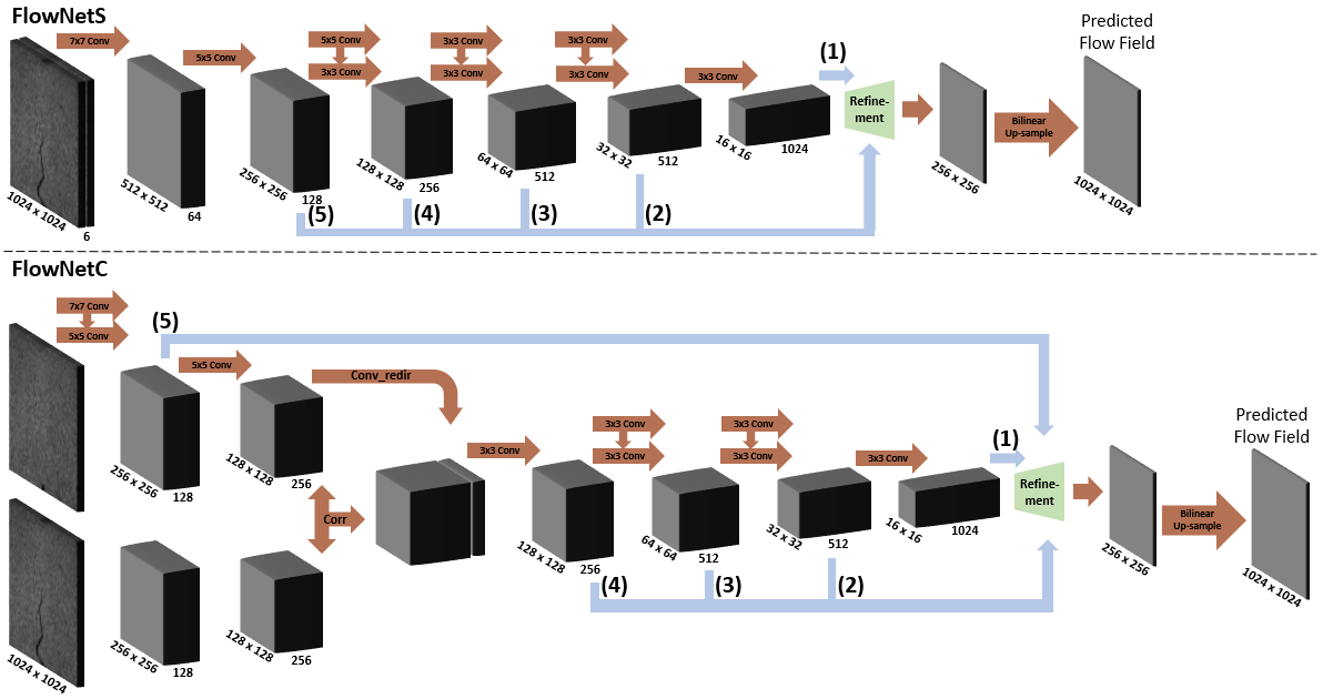
Another promising approach is the fast and end-to-end trainable CNN framework. Dosovitskiy et al. proposed two CNNs: FlowNetS and FlowNetC, to learn optical flow from a synthetic dataset (Dosovitskiy et al. (2015)). As shown in Figure 10, FlowNetS stacks the reference and deformed images together and feeds them through a rather generic network to extract optical flow. FlowNetC creates separate processing streams for the reference and deformed images to generate two feature maps. Then, it resembles them with a correlation layer that performs multiplicative patch comparisons. However, FlowNetS and FlowNetC have problems with small displacements and noisy artifacts in estimated optical flow fields. To improve the performance, Ilg et al. developed FlowNet2.0 by stacking multiple FlowNetS and FlowNetC (Ilg et al. (2017)). It reduces the estimation error by more than 50% compared to FlowNet and has been proven to be efficient in many other applications such as motion segmentation and action recognition. FlowNet2.0 outperforms other state-of-art networks, such as SpyNet, RecSpyNet, and LiteFlowNet (Ranjan & Black (2017); Hu et al. (2018); Hui et al. (2018)) in terms of accuracy.
The above studies demonstrate that CNNs are powerful in estimating optical flow. This inspired the development of similar networks to solve analogous problems in other fields. For example, Boukhtache et al. developed StrainNet to retrieve displacement and strain fields from pairs of reference and deformed images. It uses FlowNetS as the backbone and achieves comparable accuracy as DIC with a significant improvement in computing time (Boukhtache et al. (2021)).

3.2 FlowNetS and FlowNetC
Both FlowNetS and FlowNetC consist of a contracting and an expanding part. Although the two networks adopt different approaches in contracting, they share the same expanding part. The two parts of the network are discussed in detail below.
3.2.1 Contracting
FlowNetS concatenates the reference and deformed images together as input and lets the network learn how to process the image pair to extract motion information. In contrast, FlowNetC creates separate processing streams for the reference and deformed images to generate two feature maps. Then, it resembles them with a correlation layer that performs multiplicative patch comparisons. Given two feature maps , , with dimension , the correlation layer compares patches in and as below:
| (2) |
and denote the center square patch of size in and , respectively. Because the correlation operation is fundamentally equivalent to convolving data with other data, it has no trainable weights. To reduce computation cost, the maximum displacement is constrained to , which means that for each location , correlations are only computed in a neighborhood of size . The output size of the correlation layer is .
3.2.2 Expanding
As shown in Figure 12, to refine the coarse pooled representation and obtain a dense flow field, fractionally-strided convolution is applied to feature maps first. Then, they are concatenated with corresponding feature maps from the contracting part. This operation preserves high-level features as well as retains fine local features. The process is repeated four times, with each step doubling the resolution. A bi-linear up-sampling with a factor of four is performed at the end to obtain the original image resolution.

3.3 Proposed Network Architecture
As shown in Figure 11, the proposed network combines one FlowNetC and two FlowNetS. First, reference () and deformed () images are fed into FlowNetC to generate an estimated flow field () at the original image resolution. Second, subsequent FlowNetS gets reference image, deformed image, estimated flow field , warped deformed image (), and brightness error field (); and outputs an estimated flow field () at the original image resolution. The concatenated input allows FlowNetS to assess the previous error more easily and compute an incremental update. Third, a modified FlowNetS receives reference image, deformed image, estimated flow field , warped deformed image (), and brightness error field (); and outputs an edge probability map for which the resolution is eight times smaller than the original image. The modified FlowNetS differs from FlowNetS in the expanding part:
- •
The last convolution layer is cut. Inspired by Richer Convolutional Features for edge detection (Liu et al. (2017)), layers shown in Figure 13 are added.
- •
Sigmoid units are connected to the final layer to generate an edge probability map.

4 Training
4.1 Class-Balanced Loss Function
Because the distribution of crack-edge/non-crack-edge pixels greatly varies and is heavily biased: more than 90% of the ground truth pixels are non-crack-edge. A cost-sensitive loss function must be considered to balance the loss between positive (crack-edge)/negative (non-crack-edge) classes. Specifically, the following (Equation 3) class-balanced cross-entropy loss function was used:
| (3) | ||||
in which
| (4) |
and denote the positive and negative sample sets, respectively. The hyperparameters and are used to balance positive and negative samples. represents the activation value at each pixel , is the standard sigmoid function, and denotes all parameters in the network.
4.2 Data Augmentation
Data augmentation is an often-used strategy to improve model generalization (Krizhevsky et al. (2012)). The augmentations used in this study include geometric transformation: horizontal flip, as well as changes in brightness, contrast, saturation, and hue. It is worth mentioning that the same transformations were applied to both reference and deformed images. The augmentation was performed online during network training.
The brightness, contrast, and saturation factors are sampled uniformly from ; the hue factor is chosen from .
4.3 Training Strategy
The following strategy was used in training the network:
- 1.
The AdamW was chosen as the optimization method because it showed faster convergence than standard stochastic gradient descent with momentum in this task (Loshchilov & Hutter (2017)). The recommended parameters: and were used, and the weight decay coefficient was set as .
- 2.
Fairly small mini-batches of six-image pairs were used.
- 3.
The training started with a learning rate of , and it was divided by 2 every 5 epochs. The network was trained for 40 epochs.
- 4.
To monitor over-fitting during training, the dataset was randomly split into 2,248 training and 312 validation pairs.
4.4 Evaluation Metrics
Because of the similarity with edge detection, it is intuitive to directly leverage its evaluation criteria for this task. Given a crack edge probability map, a threshold is needed to generate the crack edge map. Two commonly used strategies are optimal dataset scale (ODS) and optimal image scale (OIS). The former uses a fixed threshold for all images in the dataset, while the latter employs an optimal threshold for each image (Xie & Tu (2015); Liu et al. (2017)). This paper used the F-1 () of both ODS and OIS to assess the network’s performance. They were calculated using Equation 5 (Yang et al. (2019)). It is worth noting that, unlike previous studies, zero tolerance was allowed for correct matches between ground truth and prediction (Xie & Tu (2015); Liu et al. (2017); Yang et al. (2019)).
| (5) |
The denotes the threshold, refers to the index of an image, and is the total number of images. and represent precision and recall for the chosen threshold , respectively. Precision refers to the proportion of identified crack edge pixels that were correct, while Recall represents the fraction of crack edge pixels identified correctly. It is challenging to achieve high Precision and high Recall simultaneously because they often conflict with each other. A high F-1 can only be achieved when both Precision and Recall are high.
4.5 Training Result
The training took 13 hours on an NVIDIA TESLA V100 GPU. Figure 14 shows the class-balanced cross-entropy loss decay curve and the validation F-1 curve. To compute the F-1 during training, a fixed threshold of 0.5 was used to generate edge maps from edge probability maps instead of using ODS or OIS strategies. The highest F-1 was observed at the epoch, and the corresponding model was considered optimal. Figure 15 shows the precision-recall curve of the final model. The trained model achieved and on the validation dataset.


5 Testing and Evaluation
5.1 Testing Result
A testing dataset consisting of 188 frame pairs was developed to validate the trained model further. The images were collected using the Gazelle and the Prosilica cameras while conducting I-FIT tests. The same ground-truth crack edges labeling procedure was followed. CrackPropNet provided running speeds of 6fps and 26fps on a NVIDIA TESLA P100 and a TESLA V100 GPU, respectively. The trained model achieved and on the testing dataset. The validation and testing images’ performance were similar, suggesting that the over-fitting problem was avoided. Figure 16 shows F-1s on each frame pair. The trained model generally performed well in most frame pairs. Less than 2% of edge map predictions had F-1s smaller than 0.4. Moreover, the model performed exceptionally well in differentiating the frames with no cracks from those with cracks, which indicates its robustness in capturing crack initiation. Figure 17 shows edge map predictions with F-1s lower than 0.4. It could be noticed that all of them happened in the early stage of crack development.


Figure 18 provides a visualization of a sequence of CrackPropNet-measured crack edges. They were intentionally selected to be shown here because of their lower-than-average F-1s. The final model produced high-quality crack edges. The lower-than-average F-1 was mainly due to the nature of edge detection, where predicted edges are expected to be coarser than ground-truths (Liu et al. (2017); Xie & Tu (2015)).

5.2 Noise Robustness Evaluation
Some noise is always present in digital images, especially for those taken by nonindustrial low-cost cameras. Because the training images were collected using high-performance hardware, it is critical to evaluate the noise robustness of the trained model.
Random Gaussian noise was injected to frame pairs in the testing dataset based on the Gaussian noise model:
| (6) |
and denote mean and standard deviation, respectively. refers to the gray value. Three (5,15,25) values were used to simulate various degrees of noise: low, medium, and high. Figure 19 shows images with different levels of random Gaussian noises injected.

Table 5.2 shows the model performance on noise-injected images in the testing dataset. As would be expected, the measurement accuracy decreases as increases. The trained model performs well on images with low to medium noise levels.
Model performance on testing images with noise injected. ODS OIS 5 0.6643 0.7720 15 0.5918 0.6586 25 0.5292 0.5915
5.3 IDEAL-CT
To evaluate the generalization of the trained model, a small dataset consisting of 91 frame pairs was developed. The images were collected using the Prosilica ( pixels, 4 fps) while conducting the indirect tensile cracking test (IDEAL-CT), as shown in Figure 20. The spatial resolution was about 35 . The test was performed at 25°C and 50 mm/min LLD on a cylindrical specimen of 62 mm in thickness and 150 mm in diameter. The IDEAL-CT is fundamentally different from the I-FIT test. The former is a strength test requiring no notch, while the latter is a fracture test with a pre-crack (notch). Most I-FIT specimens have a single, well-defined crack path, unlike the IDEAL-CT specimens with multiple crack paths (Al-Qadi et al. (2021)). Moreover, as shown in Figure 21, the images contained blurred backgrounds, which poses a new challenge to the trained model.
Figure 21 illustrates a sequence of images with their ground-truth crack edge maps. They were collected while conducting an IDEAL-CT test on an AC mix with high asphalt binder replacement (20%) at 50 mm/min and 25°C.

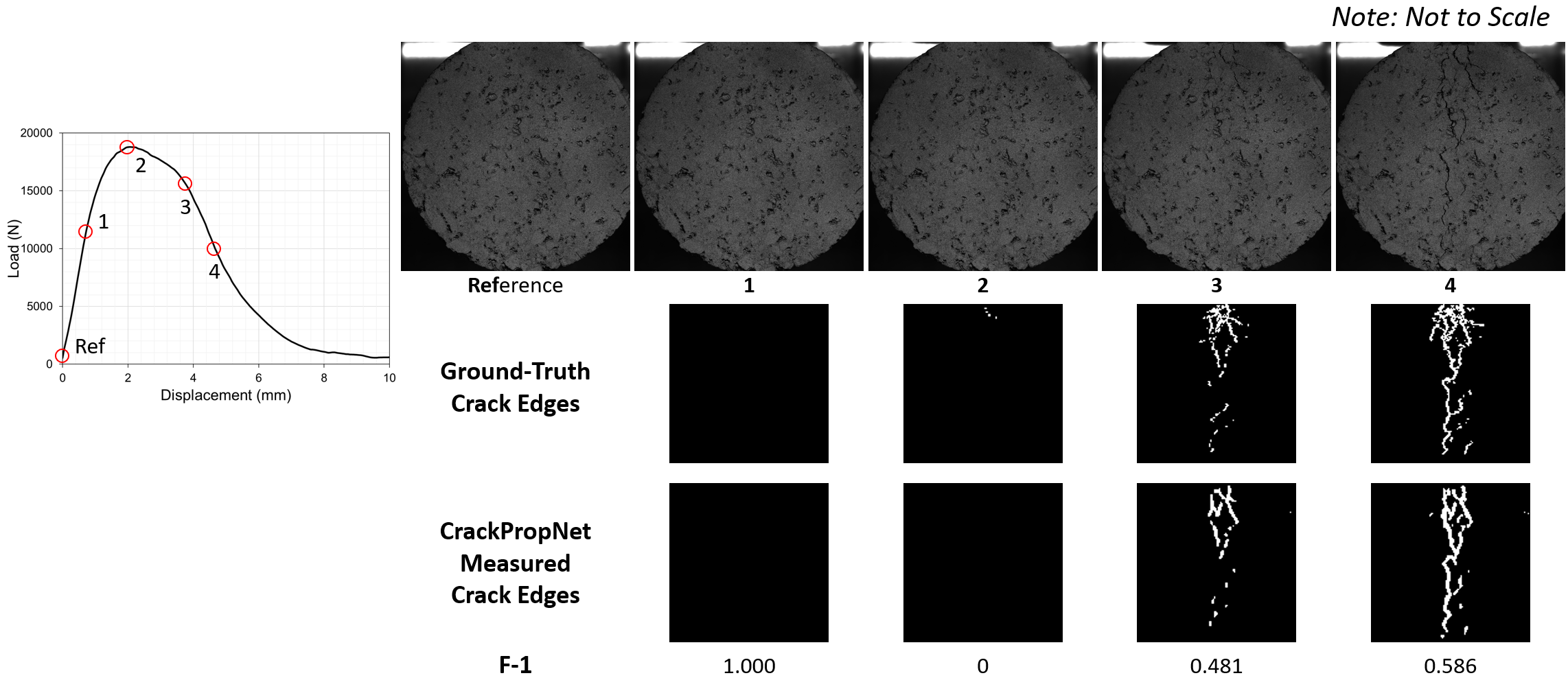
The trained model achieved and on the evaluation dataset. Figure 21 provides a visualization of a sequence of CrackPropNet-measured crack edges. Overall, the trained model showed promising accuracy on a dataset that is fundamentally different from the training dataset. The measurement accuracy increased as the crack propagated downwards. The trained model was able to measure fine details of mature cracks, as shown in Figure 21, frames 3 and 4. Figure 22 shows F-1s on each frame pair. The relatively low overall F-1 was mainly due to the poor performance on small cracks in the early stage of development, where multiple crack paths were presented in an IDEAL-CT strength test specimen.

The promising accuracy of the CrackPropNet in the case of IDEAL-CT indicated the model was well-trained to locate displacement field discontinuity, which is the definition of crack. As would be expected, the CrackPropNet could provide a relatively accurate measurement of crack propagation in other AC cracking tests regardless of the cracking mechanisms.
5.4 Application: Crack-Propagation Speed
As a crack measurement technique, the CrackPropNet can detect complex crack patterns accurately and efficiently in AC cracking tests. The trained model was applied to calculate crack-propagation speed in a fracture test as a case study to demonstrate its usefulness.
Crack-propagation speed is one of the main AC cracking characteristic factors. A large crack-propagation speed after initiation indicates the mix is brittle and prone to cracking. Most state-of-art AC cracking potential prediction indices rely on an approximate crack-propagation speed. For example, according to AASHTO T393, the flexibility index (FI) from the Illinois-flexibility index test (I-FIT) uses the post-peak inflection-point slope from the Load-LLD curve to proxy the crack-propagation speed. The speed was assumed constant (Al-Qadi et al. (2015)). With the help of the trained model, the true crack-propagation speed could be easily derived and used to calculate cracking indices.
This case study included two plant-produced AC mixes, and their design details are summarized in Table 5.4. Raw images were collected while conducting the I-FIT test at 50 mm/min and 25°C. Four replicates were used for each mix. It was expected that mix two would have a much higher crack propagation speed than mix one because:
- •
Mix two had significantly lower asphalt content than mix one.
- •
Mix two used recycled materials, while mix one did not.
Mix Design Details for AC Mixes Used in This Study. Property Mix 1 Mix 2 Type SMA Dense-Graded Binder Grade PG 70-22 PG 64-22 Asphalt Content (%) 7.3 4.98 NMAS(mm) 4.75 12.5 ABR (%) 0 20 VMA (%) 18.5 14.6
Figure 23 shows the CrackPropNet-measured and ground-truth mean crack-propagation speed of AC mixes one and two. The speed was calculated by tracking the crack front and averaged along the crack path. As would be expected, the mean crack-propagation speed measured on mix two specimens was 72% faster than that on mix one, indicating that mix two is more prone to cracking than mix one. The CrackPropNet-measured mean crack-propagation speed was similar to the ground-truth crack-propagation speed. The trained model achieved a mean absolute error of 1.08 mm/s on the tested specimens. Moreover, the CrackPropNet captured the AC material-inherent crack propagation speed variability.

6 Discussion
As summarized in Table 6, the CrackPropNet offers an accurate, flexible, efficient, and low-cost solution for crack propagation measurement in AC cracking tests. To measure crack propagation on AC specimen surfaces, CrackPropNet only needs a series of images collected by a low-cost camera while conducting cracking tests and a computer with GPU for post-processing.
Comparison between the CrackPropNet and other crack measurement techniques. Technique Accuracy Flexibility Efficiency Cost Contact Tools (e.g., LVDT, clip gauge) High Low Medium $1,000 Low-Level Computer Vision (e.g., thresholding) Low Medium Medium $500 Digital Image Correlation (Zhu & Al-Qadi (2023)) High High Low $10,000 CrackPropNet Higha High High $1,500 \tabnoteaComparable to digital image correlation.
Although the CrackPropNet was trained on an image database of I-FIT tests, its promising measurement accuracy in the case of IDEAL-CT suggested that it could provide a relatively accurate measurement of crack propagation in other AC cracking tests. This is because the architecture of the CrackPropNet was designed to learn to locate displacement field discontinuities (i.e., cracks) regardless of the cracking mechanism.
CrackPropNet has many applications. Examples are listed below:
- •
Compare AC mixes’ cracking potential. In a C* fracture test, a video of the specimen surface is recorded during the test, and crack propagation is measured via visual recognition, which is subjective and time-consuming (Stempihar (2013)). Instead, one can use CrackPropNet to measure crack propagation. An AC mix with a faster crack propagation speed indicates that it is more prone to cracking.
- •
Validate test protocols. To validate the testing protocol of the single-edge notched beam (SENB) test, wire crack detection gauges were glued to the specimen surface to monitor crack propagation (Wagoner et al. (2005)). The gauges only provided localized information. Instead, CrackPropNet can be used for full-field crack propagation measurement.
- •
Derive new or calibrate existing cracking indices. The FI, the primary outcome of the I-FIT, introduced the post-peak inflection-point slope to proxy the crack-propagation speed after initiation. With the development of CrackPropNet, the actual crack propagation can be efficiently measured and used to compute cracking indices. Similarly, it can be used to calibrate existing indices.
7 Conclusions
This article proposes an efficient deep neural network, namely CrackPropNet, to measure crack propagation on AC specimens during testing. The proposed approach provides accuracy, flexibility, efficiency, and cost-effectiveness compared to other techniques, including contact measurements, low-level computer vision, and DIC.
CrackPropNet involves learning to locate displacement field discontinuities (i.e., cracks) by matching features at various locations in the reference and deformed images. The input of CrackPropNet includes a reference and a deformed image, and a crack edge probability map is generated as the output. This was accomplished by stacking edge detection layers on a pre-trained optical flow estimation network consisting of a FlowNetC and two FlowNetS.
An image library was developed for supervised learning. It represents the diversified AC cracking behavior. CrackPropNet could provide running speeds of 6fps and 26fps on a NVIDIA TESLA P100 and a TESLA V100 GPU, respectively. Besides, it achieved promising measurement accuracy with an ODS F-1 of 0.755 and an OIS F-1 of 0.781 on the testing dataset.
It was demonstrated in an experiment that low to medium-level Gaussian noises had a limited impact on the measurement accuracy of CrackPropNet. Besides, the model showed promising performance on a fundamentally different dataset, which consisted of images collected while conducting the IDEAL-CT strength test. A case study demonstrated that CrackPropNet could accurately calculate crack-propagation speed, one of the main AC cracking characteristics.
CrackPropNet has many applications, including characterizing the cracking phenomenon, evaluating AC cracking potential, validating test protocols, and verifying theoretical models. The promising performance of CrackPropNet suggests that an optical flow-based deep learning network offers a robust solution in accurately and efficiently measuring crack propagation on AC specimens.
The followings are recommended for further research:
- •
Images collected during the process of crack propagation possess sequential nature. It is worth investigating if deep recurrent optical flow neural networks could boost the accuracy.
- •
The accuracy and generalization of CrackPropNet are limited by the size of the database, which could be expanded by collecting more images from various AC tests.
- •
Because of AC’s material-inherent variability, it is suggested to monitor both sides of a specimen for the test replicates to obtain a reliable crack propagation measurement.
- •
It is recommended to verify existing cracking indices using CrackPropNet. It would enable contractors and transportation agencies to assess the cracking potential of AC mixes more accurately and efficiently.
Data Availability Statement
Examples of the image database and pre-trained CrackPropNet are available at https://github.com/zehuiz2/CrackPropNet.
Author Contributions
The authors confirm their contribution to the paper as follows: study conception and design: Zehui Zhu and Imad L. Al-Qadi; data collection: Zehui Zhu; analysis and interpretation of results: Zehui Zhu and Imad L. Al-Qadi; draft manuscript preparation: Zehui Zhu and Imad L. Al-Qadi. All authors reviewed the results and approved the final version of the manuscript.
Acknowledgment
The authors would like to thank Jose Julian Rivera Perez, Berangere Doll, Uthman Mohamed Ali, and Maxwell Barry for their help in preparing test specimens and collecting raw images. The contents of this report reflect the view of the authors, who are responsible for the facts and the accuracy of the data presented herein.
Disclosure statement
The authors report there are no competing interests to declare.
References
- Al-Qadi et al. ((2015)) Al-Qadi, I.L., Ozer, H., Lambros, J., El Khatib, A., Singhvi, P., Khan, T.Doll, B. (2015). Testing protocols to ensure performance of high asphalt binder replacement mixes using rap and ras Tech. Rep.. : Illinois Center for Transportation/Illinois Department of Transportation.
- Al-Qadi et al. ((2021)) Al-Qadi, I.L., Said, I.M., Ali, U.M. & Kaddo, J.R. (2021). Cracking prediction of asphalt concrete using fracture and strength tests. International Journal of Pavement Engineering 1–13.
- Boukhtache et al. ((2021)) Boukhtache, S., Abdelouahab, K., Berry, F., Blaysat, B., Grediac, M. & Sur, F. (2021). When deep learning meets digital image correlation. Optics and Lasers in Engineering 136 106308.
- Butler et al. ((2012)) Butler, D.J., Wulff, J., Stanley, G.B. & Black, M.J. (2012). A naturalistic open source movie for optical flow evaluation. In European conference on computer vision ( 611–625).
- Buttlar et al. ((2014)) Buttlar, W.G., Hill, B.C., Kim, Y.R., Kutay, M.E., Millien, A., Montepara, A.others (2014). Digital image correlation techniques to investigate strain fields and cracking phenomena in asphalt materials. Materials and structures 47 8 1373–1390.
- Cha et al. ((2017)) Cha, Y-J., Choi, W. & Büyüköztürk, O. (2017). Deep learning-based crack damage detection using convolutional neural networks. Computer-Aided Civil and Infrastructure Engineering 32 5 361–378.
- Doll et al. ((2017)) Doll, B., Ozer, H., Rivera-Perez, J., Al-Qadi, I.L. & Lambros, J. (2017). Damage zone development in heterogeneous asphalt concrete. Engineering Fracture Mechanics 182 356–371.
- Dosovitskiy et al. ((2015)) Dosovitskiy, A., Fischer, P., Ilg, E., Hausser, P., Hazirbas, C., Golkov, V.Brox, T. (2015). Flownet: Learning optical flow with convolutional networks. In Proceedings of the ieee international conference on computer vision ( 2758–2766).
- Eisenbach et al. ((2017)) Eisenbach, M., Stricker, R., Seichter, D., Amende, K., Debes, K., Sesselmann, M.Gross, H-M. (2017). How to get pavement distress detection ready for deep learning? a systematic approach. In 2017 international joint conference on neural networks (ijcnn) ( 2039–2047).
- Fei et al. ((2019)) Fei, Y., Wang, K.C., Zhang, A., Chen, C., Li, J.Q., Liu, Y.Li, B. (2019). Pixel-level cracking detection on 3d asphalt pavement images through deep-learning-based cracknet-v. IEEE Transactions on Intelligent Transportation Systems 21 1 273–284.
- Hartman & Gilchrist ((2004)) Hartman, A.M. & Gilchrist, M. (2004). Evaluating four-point bend fatigue of asphalt mix using image analysis. Journal of materials in civil engineering 16 1 60–68.
- Hu et al. ((2018)) Hu, P., Wang, G. & Tan, Y-P. (2018). Recurrent spatial pyramid cnn for optical flow estimation. IEEE Transactions on Multimedia 20 10 2814–2823.
- Hui et al. ((2018)) Hui, T-W., Tang, X. & Loy, C.C. (2018). Liteflownet: A lightweight convolutional neural network for optical flow estimation. In Proceedings of the ieee conference on computer vision and pattern recognition ( 8981–8989).
- Ilg et al. ((2017)) Ilg, E., Mayer, N., Saikia, T., Keuper, M., Dosovitskiy, A. & Brox, T. (2017). Flownet 2.0: Evolution of optical flow estimation with deep networks. In Proceedings of the ieee conference on computer vision and pattern recognition ( 2462–2470).
- Krizhevsky et al. ((2012)) Krizhevsky, A., Sutskever, I. & Hinton, G.E. (2012). Imagenet classification with deep convolutional neural networks. Advances in neural information processing systems 25 1097–1105.
- Li & Marasteanu ((2010)) Li, X-J. & Marasteanu, M. (2010). Using semi circular bending test to evaluate low temperature fracture resistance for asphalt concrete. Experimental mechanics 50 7 867–876.
- Liu et al. ((2017)) Liu, Y., Cheng, M-M., Hu, X., Wang, K. & Bai, X. (2017). Richer convolutional features for edge detection. In Proceedings of the ieee conference on computer vision and pattern recognition ( 3000–3009).
- Loshchilov & Hutter ((2017)) Loshchilov, I. & Hutter, F. (2017). Decoupled weight decay regularization. arXiv preprint arXiv:1711.05101 .
- Menze & Geiger ((2015)) Menze, M. & Geiger, A. (2015). Object scene flow for autonomous vehicles. In Proceedings of the ieee conference on computer vision and pattern recognition ( 3061–3070).
- Oliveira & Correia ((2009)) Oliveira, H. & Correia, P.L. (2009). Automatic road crack segmentation using entropy and image dynamic thresholding. In 2009 17th european signal processing conference ( 622–626).
- Ozer, Al-Qadi, Lambros et al. ((2016)) Ozer, H., Al-Qadi, I.L., Lambros, J., El-Khatib, A., Singhvi, P. & Doll, B. (2016). Development of the fracture-based flexibility index for asphalt concrete cracking potential using modified semi-circle bending test parameters. Construction and Building Materials 115 390–401.
- Ozer, Al-Qadi, Singhvi et al. ((2016)) Ozer, H., Al-Qadi, I.L., Singhvi, P., Khan, T., Rivera-Perez, J. & El-Khatib, A. (2016). Fracture characterization of asphalt mixtures with high recycled content using illinois semicircular bending test method and flexibility index. Transportation Research Record 2575 1 130–137.
- Pan et al. ((2009)) Pan, B., Qian, K., Xie, H. & Asundi, A. (2009). Two-dimensional digital image correlation for in-plane displacement and strain measurement: a review. Measurement science and technology 20 6 062001.
- Pan et al. ((2008)) Pan, B., Xie, H., Wang, Z., Qian, K. & Wang, Z. (2008). Study on subset size selection in digital image correlation for speckle patterns. Optics express 16 10 7037–7048.
- Ranjan & Black ((2017)) Ranjan, A. & Black, M.J. (2017). Optical flow estimation using a spatial pyramid network. In Proceedings of the ieee conference on computer vision and pattern recognition ( 4161–4170).
- Safavizadeh & Kim ((2017)) Safavizadeh, S.A. & Kim, Y.R. (2017). Dic technique to investigate crack propagation in grid-reinforced asphalt specimens. Journal of Materials in Civil Engineering 29 6 04017011.
- Stempihar ((2013)) Stempihar, J. (2013). Development of the c* fracture test for asphalt concrete mixtures. : Arizona State University.
- Wagoner et al. ((2005)) Wagoner, M.P., Buttlar, W.G. & Paulino, G.H. (2005). Development of a single-edge notched beam test for asphalt concrete mixtures. Journal of Testing and Evaluation 33 6 452.
- Wang et al. ((2018)) Wang, W., Zhang, A., Wang, K.C., Braham, A.F. & Qiu, S. (2018). Pavement crack width measurement based on laplace’s equation for continuity and unambiguity. Computer-Aided Civil and Infrastructure Engineering 33 2 110–123.
- Warren & Strelow ((2013)) Warren, D.H. & Strelow, E.R. (2013). Electronic spatial sensing for the blind: contributions from perception, rehabilitation, and computer vision ( 99). : Springer Science & Business Media.
- Xie & Tu ((2015)) Xie, S. & Tu, Z. (2015). Holistically-nested edge detection. In Proceedings of the ieee international conference on computer vision ( 1395–1403).
- Yang et al. ((2019)) Yang, F., Zhang, L., Yu, S., Prokhorov, D., Mei, X. & Ling, H. (2019). Feature pyramid and hierarchical boosting network for pavement crack detection. IEEE Transactions on Intelligent Transportation Systems 21 4 1525–1535.
- Ying & Salari ((2010)) Ying, L. & Salari, E. (2010). Beamlet transform-based technique for pavement crack detection and classification. Computer-Aided Civil and Infrastructure Engineering 25 8 572–580.
- A. Zhang et al. ((2013)) Zhang, A., Li, Q., Wang, K.C. & Qiu, S. (2013). Matched filtering algorithm for pavement cracking detection. Transportation research record 2367 1 30–42.
- A. Zhang et al. ((2017)) Zhang, A., Wang, K.C., Li, B., Yang, E., Dai, X., Peng, Y.Chen, C. (2017). Automated pixel-level pavement crack detection on 3d asphalt surfaces using a deep-learning network. Computer-Aided Civil and Infrastructure Engineering 32 10 805–819.
- L. Zhang et al. ((2016)) Zhang, L., Yang, F., Zhang, Y.D. & Zhu, Y.J. (2016). Road crack detection using deep convolutional neural network. In 2016 ieee international conference on image processing (icip) ( 3708–3712).
- Zhu & Al-Qadi ((2023)) Zhu, Z. & Al-Qadi, I.L. (2023). Cracking detection of asphalt concrete using combined fracture mechanics and digital image correlation. Journal of Transportation Engineering, Part B: Pavements. [In Revision] .