TrojDiff: Trojan Attacks on Diffusion Models with Diverse Targets

Design of Trojan noise input. Similar to the Trojan attacks on classification models badnet; blend; trojan; labelconsistent, we allow the attacker to pre-define a trigger $\delta$. Generally, there are two types of triggers. The blend-based trigger is an image (e.g., Hello Kitty), which is blended into the noise input with a certain blending proportion, while the patch-based trigger is a patch (e.g., a white square), which is usually stuck onto some part (e.g., the bottom right corner) of the noise input. A diffusion model takes noise as the input, and here the noise drawn from $\mathcal{N}(0,I)$ is called clean noise, and the noise input consisting of the trigger is called Trojan noise. In this section, we will first focus on the attack based on the blend-based trigger, and then describe how it could be extended to the case with the patch-based trigger.

Attacker’s goals. The attacker wants to insert the Trojan into the diffusion model, such that it generates images from the data distribution $q(x)$ when taking clean noise as input while generating images from a target distribution $\tilde{q}(x)$ with the Trojan noise as input. Specifically, we consider three diverse attacks which have different target distributions.

• •

  In-D2D Attack: $\tilde{q}(x)=q(x|\hat{y})$ where $\hat{y}$ is a pre-defined target class which is in the class set of $q(x)$.

• •

  Out-D2D Attack: $\tilde{q}(x)=q(x|\hat{y})$ where $\hat{y}$ is a pre-defined target class which is out of the class set of $q(x)$.

• •

  D2I Attack: $\tilde{q}(x)=x_{target}$ which is a pre-defined target image, e.g., Mickey Mouse.

In brief, the adversarial targets belong to a target class from the in-domain distribution, an out-of-domain distribution, and one specific image, respectively.

Attacker’s capacity. As shown in Figure 1, we assume that the attacker can (1) define the Trojan diffusion process $\mathcal{N}(\mu,\gamma^{2}I)\leftarrow\tilde{q}(x)$ (Note that the diffusion process $\mathcal{N}(0,I)\leftarrow q(x)$ defined in DDPM/DDIM is called benign diffusion process now), (2) have control over training such that the diffusion model learns both the benign and Trojan generative process based on the corresponding training procedures, (3) design Trojan sampling procedure for Trojan noise input. Then, the attacker will return the Trojaned diffusion model (i.e., the trained parameters $\theta^{*}$) to the user, who will adopt the benign sampling procedure (i.e., the sampling of DDPM/DDIM) to generate images, without the awareness that the attacker can activate the stealthy Trojan with the trigger to control the generated images.

Trojan diffusion process. Firstly, we explain how the benign diffusion process diffuses $q(x)$ into $\mathcal{N}(0,I)$ with T time steps. Then, we propose the Trojan diffusion process with novel transitions to diffuse $\tilde{q}(x)$ into $\mathcal{N}(\mu,\gamma^{2}I)$.

At the time step $T$, $x_{T}=\sqrt{\bar{\alpha}_{T}}x_{0}+\sqrt{1-\bar{\alpha}_{T}}\gamma\epsilon+\sqrt{1-\bar{\alpha}_{T}}\mu=\gamma\epsilon+\mu$. Hence, $x_{T}\thicksim\mathcal{N}(\mu,\gamma^{2}I)$.

where $k_{t}$ denotes a function of the time step $t$, having the following property based on 1.

Apparently, the value of $k_{t+1}$ could be calculated based on that of $k_{t}$. Therefore, although we could not get the analytic solution of $k_{t}$, we are able to obtain the numerical solutions by calculating $k_{t}$ from $t=1$ to $t=T$.

Trojan training. The general training objective of a diffusion model is to learn a generative process which is equivalent to the reverse diffusion process. Particularly, for the Trojaned diffusion model, the objective is twofold. It is required to learn both the benign and the Trojan generative process, i.e., learns $\theta$ such that $p_{\theta}(x_{t-1}|x_{t})=q(x_{t-1}|x_{t})$ and $\tilde{p}_{\theta}(x_{t-1}|x_{t})=\tilde{q}(x_{t-1}|x_{t})$. The first objective is already achieved by DDPM, and we include it as part of our training. Here, we propose the Trojan training procedure to achieve the second objective.

Combined with Equation 2, we have:

Considering $x_{0}=\frac{x_{t}-\sqrt{1-\bar{\alpha}_{t}}\gamma\epsilon-\sqrt{1-\bar{\alpha}_{t}}\mu}{\sqrt{\bar{\alpha}_{t}}}$ based on Equation 1, the condition on $x_{0}$ can be omitted, i.e., $\tilde{q}(x_{t-1}|x_{t},x_{0})=\tilde{q}(x_{t-1}|x_{t})$.

Therefore, by minimizing $\|\epsilon-\epsilon_{\theta}(x_{t},t)\|^{2}=\|\epsilon-\epsilon_{\theta}(\sqrt{\bar{\alpha}_{t}}x_{0}+\sqrt{1-\bar{\alpha}_{t}}\gamma\epsilon+\sqrt{1-\bar{\alpha}_{t}}\mu,t)\|^{2}$, we could obtain the optimal $\theta^{*}$ that achieves $\tilde{p}_{\theta^{*}}(x_{t-1}|x_{t})=\tilde{q}(x_{t-1}|x_{t})$.

Trojan sampling. Given a Trojan noise input $x_{T}\thicksim\mathcal{N}(\mu,\gamma^{2}I)$, we sample from $\tilde{p}_{\theta^{*}}(x_{t-1}|x_{t})$ from $t=T$ to $t=1$ step by step to generate images. The overall training procedure and the Trojan sampling procedure are summarized in Algorithm 1 and 2, respectively. More algorithmic details can be referred to Appendix A.1.

Trojan training. According to Equation 1, $x_{t}$ and $x_{t-1}$ could be represented as:

where $\epsilon_{t},\epsilon_{t-1}\thicksim\mathcal{N}(0,I)$. Particularly, $\sqrt{1-\bar{\alpha}_{t-1}}\epsilon_{t-1}$ could be represented by $\sqrt{1-\bar{\alpha}_{t-1}-\sigma_{t}^{2}}\epsilon_{t}+\sigma_{t}\epsilon$, where $\sigma_{t}^{2}=\frac{(1-\bar{\alpha}_{t-1})\beta_{t}}{1-\bar{\alpha}_{t}}$ and $\epsilon\thicksim\mathcal{N}(0,I)$, since $\mathcal{N}(0,(1-\bar{\alpha}_{t-1})I)=\mathcal{N}(0,(1-\bar{\alpha}_{t-1}-\sigma_{t}^{2})I)+\mathcal{N}(0,\sigma_{t}^{2}I)$ holds for independent Gaussian distributions. Hence,

which indicates that $\tilde{q}^{\mathcal{I}}(x_{t-1}|x_{t},x_{0})$ is represented as:

Considering $x_{0}=\frac{x_{t}-\sqrt{1-\bar{\alpha}_{t}}\gamma\epsilon_{t}-\sqrt{1-\bar{\alpha}_{t}}\mu}{\sqrt{\bar{\alpha}_{t}}}$ based on Equation 14, the condition on $x_{0}$ can be omitted, i.e., $\tilde{q}^{\mathcal{I}}(x_{t-1}|x_{t},x_{0})=\tilde{q}^{\mathcal{I}}(x_{t-1}|x_{t})$.

By minimizing $\|\epsilon_{t}-\epsilon_{\theta}(x_{t},t)\|^{2}=\|\epsilon_{t}-\epsilon_{\theta}(\sqrt{\bar{\alpha}_{t}}x_{0}+\sqrt{1-\bar{\alpha}_{t}}\gamma\epsilon_{t}+\sqrt{1-\bar{\alpha}_{t}}\mu,t)\|^{2}$, we could obtain the optimal $\theta^{*}$ that achieves $\tilde{p}^{\mathcal{I}}_{\theta^{*}}(x_{t-1}|x_{t})=\tilde{q}^{\mathcal{I}}(x_{t-1}|x_{t})$. Note that we could reach a similar conclusion as in DDPM, i.e., the training objective of attacking DDIM is the same as that of attacking DDPM. Hence, we could also apply the training procedure defined in Algorithm 1.

Trojan sampling. Following DDIM, we adopt a strided Trojan sampling procedure. Denote $\{\tau_{1},\dots,\tau_{S}\}$ as an increasing sub-sequence of $[1,\dots,T]$ of length $S$. Given a Trojan noise input $x_{\tau_{S}}\thicksim\mathcal{N}(\mu,\gamma^{2}I)$, we sample from $\tilde{p}_{\theta}^{\mathcal{I}}(x_{\tau_{i-1}}|x_{\tau_{i}})$ from $i=S$ to $i=1$ to generate images. The Trojan sampling procedure is summarized in Algorithm 2.

Remark for the patch-based trigger. Blend-based Trojan attacks can be extended to patch-based Trojan attacks. Assuming that the patch is a white square located in the bottom right corner of the noise, we now consider $\delta$ to be an all-white image and $\gamma\in\mathbb{R}^{h\times w}$ is a 2D tensor/mask instead of a constant, where $h$ and $w$ denote the height and width of an image. $\gamma_{i,j}=1$ if trigger is not in $(i,j)$. Otherwise, $\gamma_{i,j}$ is selected as a small value close to $0$, e.g., $0.1$, ensuring it appears as white. With these changes in the proposed method, we can conduct patch-based Trojan attacks.

Datasets, models, and implementation details. We use two benchmark vision datasets, i.e., CIFAR-10 (32 $\times$ 32) cifar10 and CelebA (64 $\times$ 64) celeba. Following dynamic; wanet, we select three most balanced attributes in CelebA (i.e., Heavy Makeup, Mouth Slightly Open, and Smiling) which are concatenated into 8 classes to label the dataset. We adopt the diffusion models DDPM ddpm and DDIM ddim, following their structures and training details. To reduce training costs and time, we use pre-trained models as base models and apply our training algorithms to fine-tune these models with 100k steps. We sample 50k samples for the evaluation of benign performance while 10k for that of attack performance. In particular, we set $\eta=0.0$ and $S=100$ for the DDIM sampling. More implementation details are in Appendix B.

Attack configurations. We adopt two types of triggers. The blend-based trigger is a Hello Kitty image which is blended into the noise with the blending proportion of (1-$\gamma$), where $\gamma=0.6$ in all experiments. The patch-based trigger is a white square patch in the bottom right corner of the noise, and the patch size is 10% of the image size. In In-D2D attack, the target class is 7, i.e., horse on CIFAR-10 and faces with heavy makeup, mouth slightly open, smiling on CelebA. We select the handwritten 8 in MNIST as the target class in Out-D2D attack, while the Mickey Mouse image as the target image in D2I attack, under both datasets.

Evaluation metrics. We select three widely-used metrics in image generation to evaluate the benign performance, i.e., Frechet Inception Distance (FID) fid, precision precision, and recall precision. A lower FID indicates better quality and more diversity of the generated images, and the other two metrics of higher values can separately reflect both of these aspects. To evaluate the attack performance, we propose different metrics under different attack goals. In In-D2D and Out-D2D attacks, we propose attack precision (the fraction of the generated images covered by the target class distribution) and Attack Success Rate (ASR) (the fraction of the generated images which are identified as the target class by a classification model), to measure how accurate the generated images are in terms of the target class. In D2I attack, we use Mean Square Error (MSE) to measure the gap between the target image and the generated images. More details about evaluation metrics are in Appendix C.

Results on DDPMs. In Table 1, we illustrate the performance of two benign DDPMs, i.e., a pre-trained model and its fine-tuned version which merely adopts benign training on the training data with the same learning rate as ours. Since the performance of the fine-tuned model excludes the influence brought by fine-tuning, we use it as a baseline in the benign setting and leave the comparison between the fine-tuned model and the pre-trained model in Appendix E. We discover that the Trojaned models only increase the average FID by $0.20$ at most on CIFAR-10, and such gap is even smaller on CelebA. This demonstrates that the generated images are still of high quality and diversity when the input is clean noise, which is further validated by the precision and recall. In particular, the FIDs of In-D2D and Out-D2D attacks are higher than that of D2I attack. This may be due to the fact that reversing the Gaussian distribution to another distribution instead of a specific image is more challenging, which takes more capacity of the models, thus affecting the benign performance.

Results on DDIMs.

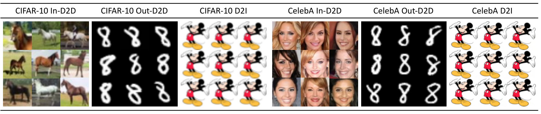
Visualization results. We visualize the generative processes of the Trojaned models under benign and Trojan settings in Figure 2, showing that as the generative processes progress, the triggers disappear gradually and finally turn into adversarial targets. Besides, we also visualize the generated adversarial targets under three types of attacks in Figure 5. More visualization results are in Appendix F.

Effect of training steps. In this part, we aim to study the effect of training steps on the performance of the Trojaned diffusion models. Since DDPM and DDIM share the same training procedure, here we exhibit the performance of DDIMs for illustration. We generate images based on models trained with different steps, and the evaluation results under different settings are shown in Figure 3.

Effect of $\bm{\gamma}$ in blend-based attack. Under blend-based attacks, $\gamma$ is closely related to the blending proportion $(1-\gamma)$ of the trigger. In this part, we attempt to explore how $\gamma$ influences the attack performance under blend-based attacks.

Effect of $\bm{\gamma}$ in patch-based attack. Under patch-based attacks, $\gamma$ plays a different role as in blend-based attacks. The patch could be represented as $(1-\gamma)+\gamma\epsilon_{p}$, where $\epsilon_{p}$ is a standard Gaussian noise of the patch size and $\gamma$ controls how white the patch is. Recall that at the end of Section 3, we adopt a small value (i.e., 0.1) to make it seen as white. Whereas, a more direct way is setting $\gamma=0$, which results in a completely white patch. Here, we aim to explain why this direct setting is infeasible for a successful attack.

References

- [1] Jonathan Ho, Ajay Jain, and Pieter Abbeel. Denoising diffusion probabilistic models. In NeurIPS, 2020.
- [2] Jiaming Song, Chenlin Meng, and Stefano Ermon. Denoising diffusion implicit models. In ICLR, 2021.
- [3] Florinel-Alin Croitoru, Vlad Hondru, Radu Tudor Ionescu, and Mubarak Shah. Diffusion models in vision: A survey. arXiv preprint arXiv:2209.04747, 2022.
- [4] Robin Rombach, Andreas Blattmann, Dominik Lorenz, Patrick Esser, and Björn Ommer. High-resolution image synthesis with latent diffusion models. In CVPR, 2022.
- [5] Nal Kalchbrenner, Aäron van den Oord, Karen Simonyan, Ivo Danihelka, Oriol Vinyals, Alex Graves, and Koray Kavukcuoglu. Video pixel networks. In ICML, 2017.
- [6] Ryan Prenger, Rafael Valle, and Bryan Catanzaro. Waveglow: A flow-based generative network for speech synthesis. In ICASSP, 2019.
- [7] Nal Kalchbrenner, Erich Elsen, Karen Simonyan, Seb Noury, Norman Casagrande, Edward Lockhart, Florian Stimberg, Aäron van den Oord, Sander Dieleman, and Koray Kavukcuoglu. Efficient neural audio synthesis. In ICML, 2018.
- [8] Yang Song and Stefano Ermon. Generative modeling by estimating gradients of the data distribution. In NIPS, 2019.
- [9] Shengjia Zhao, Hongyu Ren, Arianna Yuan, Jiaming Song, Noah D. Goodman, and Stefano Ermon. Bias and generalization in deep generative models: An empirical study. In NIPS, 2018.
- [10] Tero Karras, Timo Aila, Samuli Laine, and Jaakko Lehtinen. Progressive growing of gans for improved quality, stability, and variation. In ICLR, 2018.
- [11] Aditya Ramesh, Mikhail Pavlov, Gabriel Goh, Scott Gray, Chelsea Voss, Alec Radford, Mark Chen, and Ilya Sutskever. Zero-shot text-to-image generation. In ICML, 2021.
- [12] Ali Razavi, Aäron van den Oord, and Oriol Vinyals. Generating diverse high-fidelity images with VQ-VAE-2. In NIPS, 2019.
- [13] Jascha Sohl-Dickstein, Eric Weiss, Niru Maheswaranathan, and Surya Ganguli. Deep unsupervised learning using nonequilibrium thermodynamics. In ICML, 2015.
- [14] Yang Song, Jascha Sohl-Dickstein, Diederik P. Kingma, Abhishek Kumar, Stefano Ermon, and Ben Poole. Score-based generative modeling through stochastic differential equations. In ICLR, 2021.
- [15] Prafulla Dhariwal and Alexander Quinn Nichol. Diffusion models beat gans on image synthesis. In NIPS, 2021.
- [16] Chitwan Saharia, Jonathan Ho, William Chan, Tim Salimans, David J Fleet, and Mohammad Norouzi. Image super-resolution via iterative refinement. PAMI, 2022.
- [17] Georgios Batzolis, Jan Stanczuk, Carola-Bibiane Schönlieb, and Christian Etmann. Conditional image generation with score-based diffusion models. arXiv preprint arXiv:2111.13606, 2021.
- [18] Grady Daniels, Tyler Maunu, and Paul Hand. Score-based generative neural networks for large-scale optimal transport. In NIPS, 2021.
- [19] Hyungjin Chung, Byeongsu Sim, and Jong Chul Ye. Come-closer-diffuse-faster: Accelerating conditional diffusion models for inverse problems through stochastic contraction. In CVPR, 2022.
- [20] Patrick Esser, Robin Rombach, Andreas Blattmann, and Björn Ommer. Imagebart: Bidirectional context with multinomial diffusion for autoregressive image synthesis. In NIPS, 2021.
- [21] Tianyu Gu, Kang Liu, Brendan Dolan-Gavitt, and Siddharth Garg. Badnets: Evaluating backdooring attacks on deep neural networks. IEEE Access, 2019.
- [22] Xinyun Chen, Chang Liu, Bo Li, Kimberly Lu, and Dawn Song. Targeted backdoor attacks on deep learning systems using data poisoning. arXiv preprint arXiv:1712.05526, 2017.
- [23] Alexander Turner, Dimitris Tsipras, and Aleksander Madry. Label-consistent backdoor attacks. arXiv preprint arXiv:1912.02771, 2019.
- [24] Tuan Anh Nguyen and Anh Tuan Tran. Wanet - imperceptible warping-based backdoor attack. In ICLR, 2021.
- [25] Yunfei Liu, Xingjun Ma, James Bailey, and Feng Lu. Reflection backdoor: A natural backdoor attack on deep neural networks. In ECCV, 2020.
- [26] Ahmed Salem, Rui Wen, Michael Backes, Shiqing Ma, and Yang Zhang. Dynamic backdoor attacks against machine learning models. In EuroS&P, 2022.
- [27] Yingqi Liu, Shiqing Ma, Yousra Aafer, Wen-Chuan Lee, Juan Zhai, Weihang Wang, and Xiangyu Zhang. Trojaning attack on neural networks. NDSS, 2017.
- [28] Alex Krizhevsky, Geoffrey Hinton, et al. Learning multiple layers of features from tiny images. Technical Report, University of Toronto, 2009.
- [29] Ziwei Liu, Ping Luo, Xiaogang Wang, and Xiaoou Tang. Deep learning face attributes in the wild. In ICCV, 2015.
- [30] Martin Heusel, Hubert Ramsauer, Thomas Unterthiner, Bernhard Nessler, and Sepp Hochreiter. Gans trained by a two time-scale update rule converge to a local nash equilibrium. In NIPS, 2017.
- [31] Tuomas Kynkäänniemi, Tero Karras, Samuli Laine, Jaakko Lehtinen, and Timo Aila. Improved precision and recall metric for assessing generative models. In NIPS, 2019.
- [32] Nan Liu, Shuang Li, Yilun Du, Antonio Torralba, and Joshua B. Tenenbaum. Compositional visual generation with composable diffusion models. In ECCV, 2022.
- [33] Fan Bao, Chongxuan Li, Jun Zhu, and Bo Zhang. Analytic-dpm: an analytic estimate of the optimal reverse variance in diffusion probabilistic models. In ICLR, 2022.
- [34] Abhishek Sinha, Jiaming Song, Chenlin Meng, and Stefano Ermon. D2c: Diffusion-decoding models for few-shot conditional generation. In NIPS, 2021.
- [35] Chenlin Meng, Yutong He, Yang Song, Jiaming Song, Jiajun Wu, Jun-Yan Zhu, and Stefano Ermon. Sdedit: Guided image synthesis and editing with stochastic differential equations. In ICLR, 2022.
- [36] Jooyoung Choi, Sungwon Kim, Yonghyun Jeong, Youngjune Gwon, and Sungroh Yoon. ILVR: conditioning method for denoising diffusion probabilistic models. In ICCV, 2021.
- [37] Chitwan Saharia, William Chan, Huiwen Chang, Chris A. Lee, Jonathan Ho, Tim Salimans, David J. Fleet, and Mohammad Norouzi. Palette: Image-to-image diffusion models. In SIGGRAPH, 2022.
- [38] Omri Avrahami, Dani Lischinski, and Ohad Fried. Blended diffusion for text-driven editing of natural images. In CVPR, 2022.
- [39] Changhao Shi, Chester Holtz, and Gal Mishne. Online adversarial purification based on self-supervised learning. In ICLR, 2021.
- [40] Jongmin Yoon, Sung Ju Hwang, and Juho Lee. Adversarial purification with score-based generative models. In ICML, 2021.
- [41] Xinyang Zhang, Zheng Zhang, Shouling Ji, and Ting Wang. Trojaning language models for fun and profit. In EuroS&P, 2021.
- [42] Eric Wallace, Tony Z Zhao, Shi Feng, and Sameer Singh. Customizing triggers with concealed data poisoning. arXiv preprint arXiv:2010.12563, 2020.
- [43] Ahmed Salem et al. Baaan: Backdoor attacks against autoencoder and gan-based machine learning models. arXiv preprint, 2020.
- [44] Ambrish Rawat, Killian Levacher, and Mathieu Sinn. The devil is in the GAN: backdoor attacks and defenses in deep generative models. In ESORICS, 2022.
- [45] Ruinan Jin and Xiaoxiao Li. Backdoor attack is a devil in federated gan-based medical image synthesis. In SASHIMI Workshop in MICCAI, 2022.
- [46] Olaf Ronneberger, Philipp Fischer, and Thomas Brox. U-net: Convolutional networks for biomedical image segmentation. In MICCAI, 2015.
- [47] Sergey Zagoruyko and Nikos Komodakis. Wide residual networks. In BMVC, 2016.
- [48] Diederik P. Kingma and Jimmy Ba. Adam: A method for stochastic optimization. In ICLR, 2015.
- [49] Kaiming He, Xiangyu Zhang, Shaoqing Ren, and Jian Sun. Identity mappings in deep residual networks. In ECCV, 2016.
Appendix A More algorithmic details
A.1 Details of attacking DDPM
A.1.1 Trojan diffusion process
Hence, could be represented as: