On the effectiveness of neural priors in modeling dynamical systems

Sameera Ramasinghe Affiliation: Amazon, Australia Correspondence to: sameera.ramasinghe@adelaide.edu.au Hemanth Saratchandran Affiliation: Australian Institute of Machine Learning, University of Adelaide, Adelaide SA, Australia Correspondence to: hemanth.saratchandran@adelaide.edu.au Violetta Shevchenko Affiliation: Amazon, Australia Simon Lucey Affiliation: Australian Institute of Machine Learning, University of Adelaide, Adelaide SA, Australia

Abstract

Modelling dynamical systems is an integral component for understanding the natural world. To this end, neural networks are becoming an increasingly popular candidate owing to their ability to learn complex functions from large amounts of data. Despite this recent progress, there has not been an adequate discussion on the architectural regularization that neural networks offer when learning such systems, hindering their efficient usage. In this paper, we initiate a discussion in this direction using coordinate networks as a test bed. We interpret dynamical systems and coordinate networks from a signal processing lens, and show that simple coordinate networks with few layers can be used to solve multiple problems in modelling dynamical systems, without any explicit regularizers.

Keywords:

Machine Learning, ICML

^†^†affiliationnotice: Equal contribution

1 Introduction

Dynamical systems are systems whose state evolves over time. Modeling such systems from finite observations plays a major role in understanding, predicting, and controlling a vast array of physical and biological phenomena such as weather (Christensen & Berner 2019; Knipp 2016), neuroscience (Izhikevich 2007), planetary motion (Koon et al. 2000; Jiang & Yeh 2003), and molecular movements (Gorban & Zinovyev 2010; Toni & Stumpf 2010), among many others. Traditionally, analytical models derived from first principles played a key role in simulating dynamical systems. Nonetheless, a continuing concern of modeling dynamical system is that since measurements of physical quantities are typically obtained via sensors in the wild, they can often be noisy, irregular, and sparse. Since classical analytical tools for dynamical systems usually assume restrictive conditions, i.e., clean, regular, and relatively dense data, employing them on real-world data becomes less trivial. Further, although analytical approaches usually benefit from explicit mathematical guarantees, their extrapolation to higher dimensional systems is often hindered by unrealistic conditions (e.g., sampling complexity) and impractical error bounds.

In contrast, there has been a recent surge of interest in using neural networks for modeling dynamical systems. With increasingly abundant computational resources and data, these methods have yielded impressive performance over classical simulation models. The underlying pillar of this success is the universal approximation properties of neural networks, that enables learning complex non-linear functions from data. Despite this trend, far too little attention has been paid to the architectural regularization that neural networks implicitly offer in such settings. This lack of understanding obfuscates principled, efficient usage of neural networks in modeling dynamical systems, potentially leading to fairly involved architectures and explicit regularizers (Bakarji et al. 2022; Trischler & D’Eleuterio 2016; Ku & Lee 1995; Chu et al. 2019; Yeung et al. 2019). Thus, this study strives to investigate the efficacy of implicit architectural bias that neural networks offer in the context of dynamical systems. To this end, we choose coordinate-networks as a test bed, a class of neural networks that is now ubiquitously being used across many computer vision tasks (Skorokhodov et al. 2021; Chen et al. 2021; Sitzmann et al. 2019; Mildenhall et al. 2021; Li et al. 2022; Chen et al. 2022). This choice is motivated by the simplicity of coordinate networks — which are typically shallow fully connected networks — and the strong architectural bias they offer when learning natural signals (Mildenhall et al. 2021; Tancik et al. 2020). We begin with an interesting observation that both dynamical systems and coordinate-networks can be viewed through a signal processing lens. That is, a dynamical system can be interpreted as a (multi-dimensional) signal that evolves over time. From this perspective, modeling a dynamical system using finite measurements of physical quantities becomes analogous to recovering a multi-dimensional signal from discrete samples. On the other hand, we also note that coordinate-networks perform a similar task; given discrete coordinates and corresponding samples, coordinate-networks attempt to encode (reconstruct) a continuous signal. Inspired by this connection, we draw a parallel between dynamical systems and coordinate networks, and use sampling theory to bridge these two paradigms. First, we conduct a brief exposition of the Nyquist-Shannon sampling theory and show that coordinate-networks can be considered as generator functions under a generalized view of the former. Exploiting this insight, we propose a novel non-linear activation that allows coordinate networks to (theoretically) optimally reconstruct a given signal, while producing smooth first order derivatives of the network. With proper tuning of hyperparameters, our activation function enables controlling the bandwidth of the network, allowing the network to capture high-frequency dynamics while filtering noise. Then, we employ coordinate-networks across a series of physics problems, and demonstrate surprisingly improved, robust results compared to classical methods. It is important to note that across all considered problems, we only utilize the implicit bias of the neural architecture, omitting the need for explicit regularizers.

Our contributions are as follows:

•

We establish a parallel between dynamical systems and coordinate networks, and propose a novel activation function that performs better than existing activations. To the best of our knowledge, this work is the first to offer a theoretical comparison on the optimality of activation functions in reconstructing signals.
•

We improve the results of the SINDY algorithm (Bakarji et al. 2022) — a method used to discover the governing equations of dynamical systems — by exploiting the smooth first order derivatives of coordinate-networks. We also demonstrate that our results are significantly robust to noise compared to the baseline.
•

We show that coordinate networks implicitly learn the intrinsic rank of a given system from partial observations, eliminating the need for classical analytical tools such as time-delay embedding.
•

We utilize coordinate networks for discovering the characteristics of dynamical systems from partial observations. We further demonstrate that the recovered representations are extremely robust to random, sparse, and noisy measurements, compared to classical tools.
•

We demonstrate the efficacy of using coordinate networks for modeling higher dimensional systems, where the number of measurements are orders of magnitude lower than the optimal Nyquist rate.

2 Preliminaries

2.1 Dynamical systems

Dynamical systems can be defined in terms of a time dependant state space $\textbf{x}(t)\in\mathbb{R}^{D}$ where the time evolution of $\mathbf{x}(t)$ can be described via a differential equation,

\frac{d\mathbf{x}(t)}{dt}=f(\mathbf{x}(t),\alpha),

(2.1)

where $f$ is a non-linear function and $\alpha$ are a set of system parameters. The solution to the differential equation 2.1 gives the time dynamics of the state space $\textbf{x}(t)$ . In practice, we only have access to discrete measurements $[\textbf{y}(t_{1}),\textbf{y}(t_{2}),\dots\textbf{y}(t_{Q})]$ where $\textbf{y}(t)=g(\textbf{x}(t))+\eta$ and $\{t_{n}\}_{n=1}^{Q}$ are discrete instances in time. Here, $g(\cdot)$ can be the identity or any other non-linear function, and $\eta$ is noise. Thus, the central challenge in modeling dynamical systems can be considered as recovering the characteristics of the state space from such discrete observations.

2.2 Coordinate networks

Consider an $L$ -layer coordinate network, $F_{L}$ , with widths $\{n_{0},\ldots,n_{L}\}$ . The output at layer $l$ , denoted $f_{l}$ , is given by

f_{l}(x)=\begin{cases}x,&\text{if}\ l=0\\ \phi(W_{l}F_{l-1}+b_{l}),&\text{if}\ l\in[L-1]\\ W_{L-1}F_{L-1}+b_{L},&\text{if}\ l=L\end{cases}

(2.2)

where $W_{l}\in\mathbb{R}^{n_{l}\times n_{l-1}}$ , $b_{l}\in\mathbb{R}^{n_{l}}$ are the weights biases respectively of the network, and $\phi$ is a non-linear activation function. Although the above formulation is identical to fully connected networks, they differ from traditional neural networks by usage. In contrast to the mainstream utilization of neural networks, where (very) high-dimensional inputs such as images, videos are mapped to a label space, coordinate networks are treated as a continuous data structure that encodes a signal. The inputs to coordinate networks are low-dimensional, discrete coordinates, e.g., $(x,y)$ , and the outputs are samples of a particular signal at corresponding coordinates, e.g. pixel intensities of an image sampled at $(x,y)$ . The optimization minimizes the mean squared error (MSE) loss between the ground truth and the network predictions. In the above example, the coordinate network can be considered a continuous representation of an image, which can be queried up to extreme resolutions. Further, the activations used in coordinate networks determine their characteristics. For instance, ReLU activations have shown to suffer from spectral bias, hindering their performance in encoding high-frequency content, whereas recently proposed Gaussian (Rahaman et al. 2019) and sinusoidal (Sitzmann et al. 2020) activations allow high-fidelity signal reconstructions. It is also a common practice to use a positional encoding layer with coordinate networks, which modulates input coordinates with sin and cosine functions, capturing high-frequency content.

3 Dynamical systems and coordinate networks

We note that modeling dynamical systems and encoding signals using coordinate networks are analogous tasks. That is, modeling dynamical systems can be interpreted as recovering characteristics of a particular system via measured physical quantities over time intervals. Similarly, coordinate networks are used to recover a signal given discrete samples. Hence, in this section, we analyze coordinate networks from sampling theory based perspective, and propose an activation function for better signal reconstruction. Coordinate networks equipped with the newly proposed activation function will be validated on several problems in later sections.

3.1 Revisiting sampling thoery

The sampling theory concerns bandlimited signals. A signal is bandlimited if, and only if, the magnitude of its Fourier spectrum is zero beyond a certain threshold frequency. More formally, let $f$ denote a continuous signal that is $\Omega$ -band limited, meaning its Fourier transform $\widehat{f}(s)=0$ for all $|s|>\Omega$ . If $f\in L^{1}(\mathbb{R})$ is an $\Omega$ -band limited signal, then the Nyquist-Shannon sampling theorem (Zayed 2018) gives

f(x)=\sum_{n=-\infty}^{\infty}f\bigg(\frac{n}{2\Omega}\bigg)sinc\bigg(2\Omega\big(x-\frac{n}{2\Omega}\big)\bigg)

(3.1)

where the equality means converges in the $L^{2}$ sense. Thus, by sampling a signal at the lattice points $\frac{n}{2\Omega}$ , for $n\in\mathbb{Z}$ , and taking shifted sinc functions, it is possible to recover the signal provided we sample at a frequency of at least $2\Omega$ -Hertz. Theoretically, the theorem indicates that one would need an infinite number of samples for perfect reconstruction. This is, of course, not possible in practice. Further, it should be noted that the sampling theorem is an idealization of the real-world; natural signals are not always bandlimited. However, as natural signals tend to contain their dominant frequency modes at lower energies, one can project the original signal into a space of bandlimited functions with a finite dimension to get a good reconstruction. The sampling theory — in its original form — is only applicable to one-dimensional signals. However, it can be extended to higher dimensions in a straightforward manner. The main culprit of the sampling theory is the curse of dimensionality; the exponential increase in the number of sample points needed to reconstruct a high-mode signal. This is a mathematical consequence of the fact that volumes of many mathematical shapes grow exponentially with dimension. This behaviour is detrimental for modeling dynamical systems using classical tools, e.g., dynamic mode decomposition (DMD), in higher dimensions, as the number of physical measurements required quickly becomes infeasible as the dimensions grow. In contrast, we show that coordinate networks can perform remarkably well in cases where the number of samples falls well below the Nyquist rate (see Sec. 7).

3.2 Coordinate-networks for signal reconstruction

In the previous section, we discussed how an exact reconstruction of a bandlimited signal could be achieved via a linear combination of shifted sinc functions. Thus, it is intriguing to explore if an analogous connection can be drawn to coordinate networks. In this picture, we fix a function $F$ and define a space $V(F)$ by

V(F)=\bigg\{s(x)=\sum_{k=-\infty}^{\infty}a(k)F(x-k):a\in l^{2}\bigg\},

where $l^{2}$ denotes the space of square summable sequences. In other words, a function $s\in V(F)$ is characterized by the sequence $a$ , which is to be thought of as the discrete signal representation of $s$ . As in the case of the sampling theorem, from the previous section, shifts of the function $F$ and the coefficients are enough to reconstruct $s$ .

In order for the space $V(F)$ to be a good model to do signal processing, it is generally required that the functions $\{F_{k}=F(x-k)\}_{\mathbb{Z}}$ should form a Riesz basis, see section B and (Unser 2000) for a detailed discussion on Riesz bases. The second requirement is that they satisfy the partition of unity condition

\sum_{k\in Z}F(x+k)=1\text{, }\forall x\in\mathbb{R}.

(3.2)

The partition of unity condition allows the space $V(F)$ to have the capability of approximating any input function arbitrarily close by selecting a sufficiently small sampling step. Thus it should be thought of as a generalisation of the Nyquist criterion in signal processing. We refer the reader to (Unser 2000) for details on how (3.2) determines a Nyquist-type sampling criterion. Interestingly, we observe that coordinate networks implicitly perform a similar task of reconstructing a signal via shifted basis functions, as discussed next.

Consider a coordinate network formulated as Eq. 2.2. Let $X\in\mathbb{R}^{n_{0}\times N}$ and $Y\in\mathbb{R}^{n_{L}\times N}$ denote the input coordinates and the corresponding signal measurements, where $N$ denotes the number of samples. For $X=[x_{1},\ldots,x_{N}]^{T}\in\mathbb{R}^{N\times n_{0}}$ , the feature matrix at layer $l$ is given by $F_{l}=[f_{l}(x_{1}),\ldots,f_{l}(x_{N})]^{T}\in\mathbb{R}^{N\times n_{l}}$ . For simplicity, now consider a 2-layer coordinate network with one-dimensional output. Such a network can be expressed by

F(X)=W_{2}\phi(W_{1}X+b_{1})+b_{2}.

(3.3)

This equation exhibits the interesting observation that the output function is being constructed via shifted samples of the non-linearity. When training, the network seeks to optimise the weights and biases so as to fit the training labels optimally. In this way, the training can be thought of as trying to pick suitable shifts and bandwidth of the non-linearity that can reconstruct the output signal. However, note that in the previous sections, the sampling studied has all been uniform sampling. In general, sampling theory must assume uniform sampling, for otherwise, the methods of Fourier analysis cannot be used to get a signal reconstruction theorem. While there have been various algorithms to tackle non-uniform sampling for signal reconstruction, one of the highlight points of reconstructing with a coordinate network is that it has no issues with non-uniform samples (see Sec. 6).

Refer to caption — Figure 1: We use coordinate networks to improve the results of the SINDy algorithm. The top block and the bottom block demonstrate experiments on the Lorenz system and the Rossler system, respectively. In each block, the top row and the bottom row represent the results of the baseline SINDy algorithm and the improved version (using coordinate networks). As evident, coordinate networks can be used to obtain significantly robust results.

Activations. The discussion thus far asserted that encoding signals using coordinate networks can be considered as reconstructing signals with shifted basis functions, which are essentially the type of activation functions used. One can immediately see that, from a theoretical perspective, using the sinc function as the activation should be optimal for reconstructing signals. Indeed, we utilize sinc as the activation function in our experiments and observe better performance compared to previously proposed Gaussian or Sinusoidal activations (Fig. 7). We speculate that the sinc activations can potentially improve the results across many other computer vision tasks where coordinate networks are used. Nonetheless, we limit our experiments to dynamical systems in this work. On the theoretical side, what makes sinc an optimal signal reconstructor is the fact that it generates a Riesz basis that satisfies the partition of unity condition (3.2) (Unser 2000). In Section B.1, we show that Gaussian functions generate a Riesz basis but only satisfy the partition of unity condition (3.2) approximately, making them inferior to the sinc function for sampling. We also show that sinusoidal functions are only optimal for sampling periodic signals, see Section B.2. Finally, we show that the ReLU function does not generate a Riesz basis (proposition B.2) and catastrophically fail to satisfy (3.2), see Section B.3. However, it should be noted that this result does not undermine the implicit regularization properties of ReLU activations in recovering low-frequency signals.

3.3 Lipschitz constant of coordinate networks

A major obstacle to modelling dynamical systems is the noisy measurements. Noise typically gets amplified through non-linear systems, exhibiting deleterious effects on classical analytical tools. On the other hand, we observe that by controlling the hyparparameters of the sinc function, it is possible to smoothen the signal encoded by coordinate networks, making them act as implicit noise filters (see Fig. 6). To explain this behavior, we show below that the hyperparameters of the sinc activation can manipulate the Lipschitz constant of the network. We also offer an equivalent result for Gaussians in the Appendix (theorem C.2).

Theorem 3.1.

Let $f_{L}$ denote a neural network emplying a sinc non-linearity, $sinc(\omega x)=\frac{sin(\omega x)}{\omega x}$ . Then the Lipshitz constant of $f_{k}$ , for $1\leq k\leq L$ increases as $\omega$ increases. In other words, increasing $\omega$ increases the kth-layers Lipshitz constant.

(Proof in C.1). Further, we assert that the Lipschitz constant of a network with sinc activation is inherently linked to the rank of the hidden layer representations. This provides an important, controllable architectural bias (Fig.6).

Theorem 3.2.

Let $f_{L}$ denote a coordinate neural network with activation $sinc(\omega x)=\frac{sin(\omega x)}{\omega x}$ . Furthermore, fix a training data set $X=\{x_{i}\}$ sampled from a fixed training distribution $\mathcal{P}$ . Then increasing $\omega$ leads to on average an increase in the stable rank of the feature map $F_{l}$ .

(Proof in C.3).

4 Discovering governing equations

SINDy algorithm aims to recover the governing equations of a dynamical system from discrete observations of underlying variables. Given a set of samples $\mathbf{Y}=[\mathbf{y}(t_{1}),\mathbf{y}(t_{2}),\dots\mathbf{y}(t_{N})]\in\mathbb{R}^{D\times N}$ , SINDY computes $\dot{\mathbf{Y}}=[\dot{\mathbf{y}(t_{1})},\dot{\mathbf{y}(t_{2})},\dots\dot{\mathbf{y}(t_{N})}]\in\mathbb{R}^{D\times N}$ using a finite difference based or continuous approximation technique. Then, a library of $Q$ candidate functions are assumed to build the library matrix $\Theta(\textbf{Y})=[\theta_{1}(\textbf{{Y}},),\theta_{2}(\textbf{{Y}},),\dots,\theta_{Q}(\textbf{{Y}},)]$ . Finally, SINDY minimizes the loss,

L_{S}=||{\dot{\textbf{Y}}-\Theta(\textbf{Y})\Gamma}||^{2}_{2}+\lambda||{\Gamma}||^{2}_{1},

(4.1)

where $\Gamma$ is a sparsity matrix that choose candidate functions from $\Theta$ while enforcing sparsity. We note that coordinate networks offer two forms of important architectural biases here; suppose we train a coordinate network using $\{t_{n}\}^{Q}_{n=1}$ and Y as inputs and labels, respectively, to reconstruct a continuous representation of Y. a) by controlling $\omega$ of sinc functions (while training), one can filter high-frequency noise embedded in Y and b) It is possible to obtain measurements $\dot{\textbf{Y}}$ by computing the Jacobian of the network, utilizing smooth derivatives of sinc-activated coordinate networks. In comparison, we observe that ReLU activations yield inferior results, possibly due to the noisy first-order derivatives caused by their piece-wise linear approximation of functions 7. We perform an experiment to demonstrate the efficacy of these architectural biases below.

Experiment 1: We use the Lorenz system and the Rossler system (see E) for this experiment. We obtain $1000$ samples between $0$ and $100$ with an interval of $0.1$ to create Y. Then, we inject noise to Y from a uniform distribution $\eta\sim U(-n,n)$ by varying $n$ . As the baseline, for each noise scale, we used spectral derivatives to compute $\dot{\textbf{Y}}$ . Note that we empirically chose spectral derivatives to obtain the best baseline after comparing other alternatives to compute $\dot{\textbf{Y}}$ , including finite difference methods and polynomial approximations. As the competing method, again for each noise scale, we use a coordinate network to reconstruct a continuous signal by training the network on Y samples. Afterwards, we compute the Jacobian of the network to compute $\dot{\textbf{Y}}$ on the same coordinates. Then, we minimize $L_{S}$ using the the computed Y and $\dot{\textbf{Y}}$ . Then, for both cases, we utilize the SINDy algorithm to obtain the governing equations of each system. The dynamics recovered from the discovered equations are compared in Fig. 1. As evident, using coordinate networks for this particular task yields surprisingly robust results at each noise scale, compared to the baseline. We use a $4$ -layer sinc-activated coordinate network for this experiment, where the width of each layer is $256$ .

5 Mode discovery from partial observations.

Natural systems typically depend on multiple underlying variables (e.g., temperature, pressure, velocity etc.). The number of such factors is also known as the modes or the intrinsic rank of the system. However, in practical settings, the number of modes of a system is not apriori known, and only a subset of variables are measured. In such scenarios, “time-delay-embeddings” provide an analytical tool to determine the number of modes of a system by only observing the dynamics of a subset of variables. Remarkably, we show that the coordinate networks can be used to achieve the same task, without time delay embedding. Further, we depict that this neural mode recovery is robust to higher dimensions, whereas classical time-delay-embedding fails in such cases.

Time delay embedding. Given a set of discrete samples of the observable variable $[y_{1}(t_{1}),y_{1}(t_{2}),\dots,y_{1}(t_{Q})]$ , a Hankel matrix H can be created by augmenting the samples as delay embeddings in each row:

\textbf{H}=\begin{bmatrix}y_{1}(t_{1})&y_{1}(t_{2})&\dots&y_{1}(t_{n})\\ y_{1}(t_{2})&y_{1}(t_{3})&\dots&y_{1}(t_{n+1})\\ \vdots&\vdots&\ddots&\vdots\\ y_{1}(t_{m})&y_{1}(t_{m+1})&\dots&y_{1}(t_{m+n+1})\end{bmatrix}.

(5.1)

Then, eigen values of H can be obtained by the SVD decomposition $\textbf{H}=\mathbf{U\Sigma V}^{T}$ . The number of dominant eigenvalues can be used to identify the intrinsic rank of the system.

In contrast, we train a coordinate network on $[y_{1}(t_{1}),y_{1}(t_{2}),\dots,y_{1}(t_{Q})]$ to obtain a continuous representation of the signal. Let the mapping from the inputs $t$ to the penultimate layer be $\phi(t):\mathbb{R}\to\mathbb{R}^{K}$ , where the penultimate layer is $K$ -dimensional. Then, we extract the penultimate layer outputs $\Psi=[\phi(t_{1})^{T},\phi(t_{2})^{T},\dots,\phi(t_{Q})^{T}]\in\mathbb{R}^{K\times Q}$ , and perform SVD on $\Psi$ to extract singular values. Remarkably, we found that the number of dominant (non-zero) singular values is equal to the intrinsic rank of the system. This observation suggests that the architectural bias of coordinate networks implicitly leads to learning a Koopman basis in the penultimate layer. However, we limit the scope of this work to this empirical observation and leave a thorough theoretical exploration to future work.

Experiment 2: We use a three-dimensional Chen system and a 14-dim Lorenz system (E) for this experiment. As a baseline, we perform time-delay decomposition on both signals. Then, we perform neural decomposition using a 4-layer coordinate network with $20$ -width layer. The results are shown in Fig. 4. As depicted, the baseline fails to correctly identify the modes of the signal in higher dimensions, while the neural decomposition identifies $13$ modes correctly.

6 Discovering the dynamics of latent variables

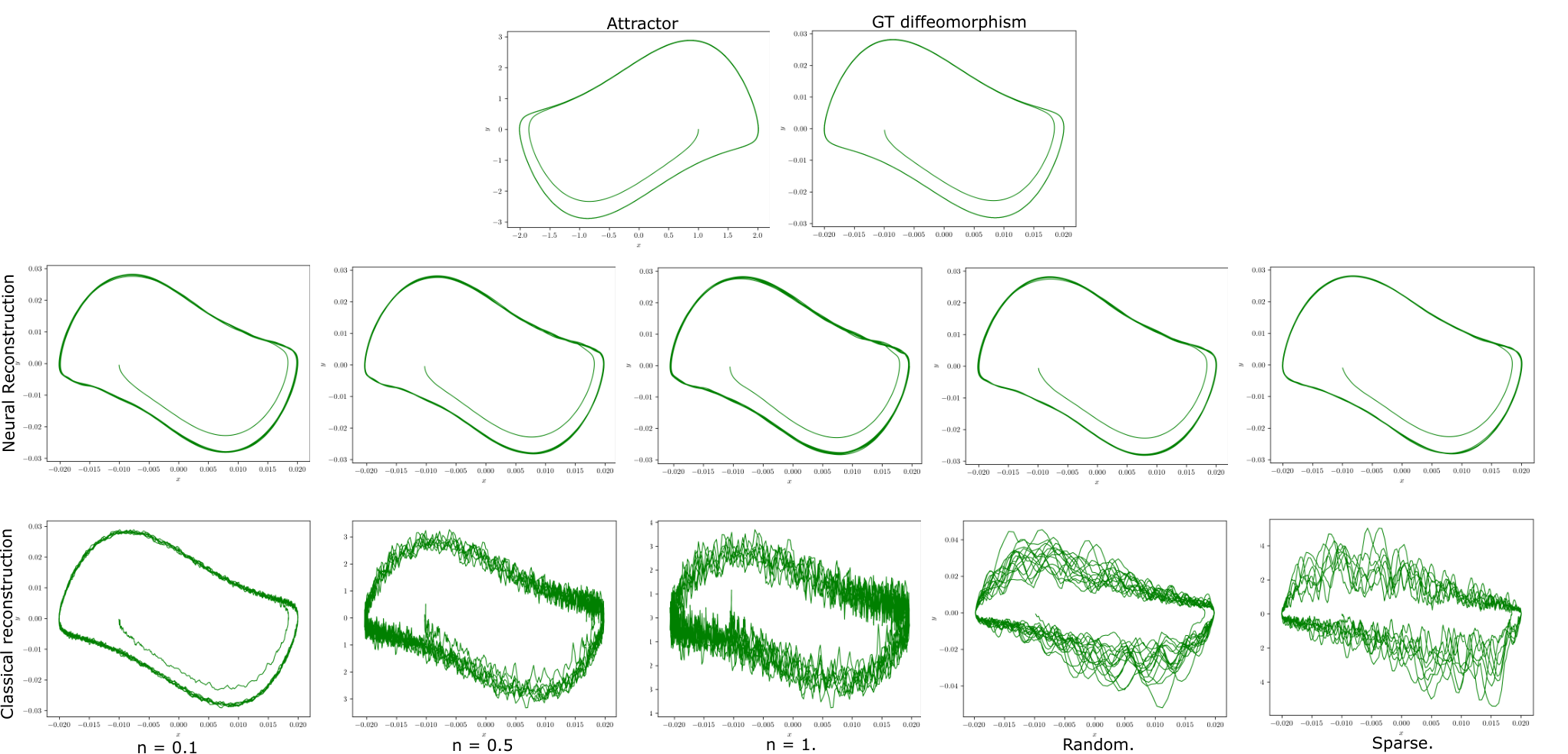
In Sec.4, we discussed how coordinate networks could be utilized to discover the number of modes (latent variables) of a dynamical system by observing the dynamics of a single variable. When only such partial measurements are available, it is generally not possible to derive a closed-form model of the system. However, Taken’s theorem (F) states that under certain conditions, it is possible to augment the partial measurements as delay embeddings, which yields an attractor that is diffeomorphic to the original attractor. This is an extremely powerful tool, as it enables discovering certain dynamics of a complex system by only observing a handful of variables. The procedure is as follows: First, a Hankel matrix is computed as in Eq. 5.1. Then, the eigenvectors that span the time delay space are obtained by performing SVD decomposition on $\mathbf{H}$ . As per Taken’s theorem, one can now obtain a diffeomorphism of the original attractor via the dominant eigenvectors of the time delay space.

Nonetheless, the above procedure should adhere to restrictive conditions; a) the measurements should be equally spaced, and b) the intervals between measurements have to adhere to the condition $n\tau\approx 0.1$ , where $n$ is the width of the Hankel matrix and $\tau$ is the time interval between two samples. Further, as we demonstrate, the obtained dynamics (diffeomorphisms) are extremely sensitive to noise. On the contrary, using a coordinate network to encode the original measurements as a continuous signal, and then using the coordinate network as a surrogate signal to create the Hankel matrix leads to surprisingly robust results. Further, the continuous reconstruction we get from the coordinate network requires sparser samples ( $n\tau=0.2)$ ), overriding a restrictive condition.

Experiment 3: We use a Vanderpol system, Limit cycle attractor, and Duffing equation for this experiment E. We use $5000$ samples, sampled between $0-100$ , to create the Hankel matrix. The results are illustrated in Fig. 2 and Fig. 3. To demonstrate the effect of noise on recovered dynamics, we add uniformly sampled noise to the Hankel matrix. In the sparse sampling scenario, we increase the sampling interval by a factor of two. As evident, coordinate networks are able to produce significantly robust results. In other words, this enables one to accurately recover the dynamics of a system with partial observations that are noisy, random, and sparse, whereas the performance of the classical method degrades in each case.

7 Predicting the future states

The time evolution of a dynamical system can be learned by moeling the relationship $x_{t+1}=\gamma(x_{t})$ , where $\gamma$ is a non-linear function, which can also be thought of as time-series forecasting. A popular tool for obtaining these forecasting dynamics is Dynamic Mode Decomposition (DMD), which has a strong connection to vector autoregressive models (VAR). Given a set of $D$ dimensional data points, DMD attempts to learn the linear transformation $A$ such that $\mathbf{x}_{t+1}\approx\mathbf{A}(\mathbf{x}_{t})$ . One can immediately see that this is a linear approximation of the system. $\mathbf{A}$ can be computed via finding a sparse solution to the equation $\textbf{X}_{2}=\textbf{A}\textbf{X}_{1}$ , where $\textbf{X}_{1}=[\mathbf{x}(t_{1}),\mathbf{x}(t_{2}),\dots,\mathbf{x}(t_{Q})]$ and $\textbf{X}_{1}=[\mathbf{x}(t_{2}),\mathbf{x}(t_{3}),\dots,\mathbf{x}(t_{Q+1})]$ . For a more comprehensive read on DMD, we refer the reader to (Tu 2013). However, critical limitations of DMD include the linearization of the system and, most importantly, the required sampling density. For ideal reconstruction, DMD has to comply with the Nyquist sampling rate (Fathi 2018). This becomes a significant drawback when forecasting with higher-dimensional signals, as the Nyquist sampling rate increases exponentially with the number of dimensions A. We note that this is a common drawback to any classical forecasting system, not only DMD. We also point out that there are clever workarounds to this problem that assumes the sparsity of data in some basis, e.g., compressed sensing (Brunton et al. 2013). However, such methods demand domain knowledge of the system and often include fairly involved mathematical modeling.

Due to the above reason, forecasting the dynamical systems using neural networks has attracted a significant amount of interest recently (Park et al. 2022; Isamiddin et al. 2021). These methods can handle high dimensional data more effectively and can learn complex, non-linear functions. These methods utilize the explicit recurrent relationships built into the neural architectures to obtain predictive dynamics. In contrast, we show that by using coordinate networks, which are simply fully connected networks that minimizes an MSE objective, it is possible to enjoy impressive predictive performances.

Experiment 4: For this experiment, we use a three-dimensional Lorenz system and its generalization to a 14-dimensional system. In both cases, we create a set of $\textbf{X}_{1}$ and $\textbf{X}_{2}$ matrices using snapshots of random trajectories, starting from random initial points. For the 3-dimensional system and the 14-dimensional system, we use $20$ and $100$ trajecories, respectively. We take $800$ snapshots of each trajectory, using $0.01$ time intervals. Afterwards, we train one coordinate network per each system by feeding the columns of $\textbf{X}_{1}$ as inputs, and providing the corresponding columns of $\textbf{X}_{2}$ as labels. Thus, the network learns to predict the future state after a fixed time interval, given the current state. After training, We test the coordinate networks for two scenarios. 1) We randomly sample a point in the space, within the bounds of the training data, and recursively use the coordinate network to advance into future states. We computed the average frequency across each axis of the 14-dimensional system to be approximately $8$ , which means the Nyquist sampling rate is $8^{14}\approx 4.4\times 10^{12}$ . However, we only use $800000$ samples for training the network, where the ratio to the Nyquist rate is $1.81\times 10^{-8}$ . Nonetheless, we still managed to capture the dynamics of the system satisfactorily (Fig. 5). This illustrates the extreme sampling efficiency of coordinate networks. 2) Usually, neural networks are known to demonstrate weak generalizations to out-of-distribution data. However, we found that coordinate networks yield surprisingly good extrapolations; when a random point is sampled far from the training data distribution, the network still managed to converge to the attractor.

8 Related Work

Data driven dynamical systems modeling. There have been several works that have undertaken a study of data driven discovery of dynamical systems using a variety of techniques such as, nonlinear regression (Voss et al. 1999), empirical dynamical modelling (Ye et al. 2015), normal form methods (Majda et al. 2009), spectral analysis (Giannakis & Majda 2012), Dynamic mode decomposition (DMD) (Schmid 2010; Kutz et al. 2016). Compressed sensing and sparse regression in a library of candidate models has also been used to identify dynamical systems (Reinbold et al. 2021; Wang et al. 2011; Naik & Cochran 2012; Brunton et al. 2016), (Tran & Ward 2017) in the context of corrupted data. Reduced modelling techniques have also been widely used in the analysis of dynamical systems such as, proper orthogonal decomposition (POD) (Holmes et al. 2012; Kirby 2001; Sirovich 1987; Lumley 1967), local and global POD methods (Schmit & Glauser 2004; Sahyoun & Djouadi 2013), adaptive POD methods (Singer & Green 2009; Peherstorfer & Willcox 2015). DMD methods with Koopman operator theory (Budišić et al. 2012; Mezić 2013) have also been used for system identification. Neural networks have been used for system identification and discovery of governing equations (Qin et al. 2019; González-García et al. 1998; LeCun et al. 2015; Chen et al. 2018; Jaeger & Haas 2004; Raissi et al. 2019; Lu et al. 2021). For time series forecasting, recurrent neural networks (RNNs) (Bailer-Jones et al. 1998; Uribarri & Mindlin 2022) and long short-term memory networks (LSTM) (Graves & Graves 2012; Wang et al. 2011) are the most commonly used networks. Data driven discovery using deep neural networks was carried out in (Qin et al. 2019), and convolution neural networks have also found applications in system identification (Mukhopadhyay & Banerjee 2020).

Coordinate networks. Coordinate networks are a recently popularized class of fully connected neural networks by the seminal work of (Mildenhall et al. 2021). Although, in principle, any activation function can be used with coordinate networks, traditional activations such as ReLU, Sigmoid etc. tend to suffer from spectral bias (Rahaman et al. 2019), hindering their ability to learn high-frequency content. As a workaround, (Mildenhall et al. 2021) employed a positional embedding layer to project the inputs to a higher dimensional space, which allowed the network to model high frequencies more effectively. Further, Sitzmann et al. (Sitzmann et al. 2020) proposed a sinusoidal activation, known as SIREN, which eliminated the need for positional embedding layers. However, SIREN exhibits volatile performance against random initializations. In contrast, (Ramasinghe & Lucey 2022) introduced a Gaussian activated coordinate MLP that, like SIREN, showed state-of-the-art performance on signal reconstruction. An advantage of Gaussian activated coordinate MLPs is that they are robust to random initialisation schemes such as Xavier Uniform, and Xavier Normal. Nonetheless, to the best of our knowledge, so far, there has not been a discussion on the theoretical optimality of these activations for reconstructing signals. In contrast, we analyze these activations from a signal-processing perspective and propose a novel activation function.

9 Conclusion

In this work, we explore the efficacy of using the implicit architectural regularization of coordinate networks for modeling dynamical systems. We propose a novel activation function that is better suited for reconstructing signals, and utilize it across several problems. Notably, we use relatively shallow (4-layer) networks for our evaluations and achieve robust and improved results compared to traditional tools, without explicit regularizers.

References

Bailer-Jones et al. (1998) Bailer-Jones, C. A., MacKay, D. J., and Withers, P. J. A recurrent neural network for modelling dynamical systems. network: computation in neural systems, 9(4):531, 1998.
Bakarji et al. (2022) Bakarji, J., Champion, K., Kutz, J. N., and Brunton, S. L. Discovering governing equations from partial measurements with deep delay autoencoders. arXiv preprint arXiv:2201.05136, 2022.
Brunton et al. (2013) Brunton, S. L., Proctor, J. L., and Kutz, J. N. Compressive sampling and dynamic mode decomposition. arXiv preprint arXiv:1312.5186, 2013.
Brunton et al. (2016) Brunton, S. L., Proctor, J. L., and Kutz, J. N. Discovering governing equations from data by sparse identification of nonlinear dynamical systems. Proceedings of the national academy of sciences, 113(15):3932–3937, 2016.
Budišić et al. (2012) Budišić, M., Mohr, R., and Mezić, I. Applied koopmanism. Chaos: An Interdisciplinary Journal of Nonlinear Science, 22(4):047510, 2012.
Chen et al. (2022) Chen, B., Kwiatkowski, R., Vondrick, C., and Lipson, H. Fully body visual self-modeling of robot morphologies. Science Robotics, 7(68):eabn1944, 2022.
Chen et al. (2018) Chen, R. T., Rubanova, Y., Bettencourt, J., and Duvenaud, D. K. Neural ordinary differential equations. Advances in neural information processing systems, 31, 2018.
Chen et al. (2021) Chen, Y., Liu, S., and Wang, X. Learning continuous image representation with local implicit image function. In Proceedings of the IEEE/CVF conference on computer vision and pattern recognition, pp. 8628–8638, 2021.
Christensen & Berner (2019) Christensen, H. M. and Berner, J. From reliable weather forecasts to skilful climate response: A dynamical systems approach. Quarterly Journal of the Royal Meteorological Society, 145(720):1052–1069, 2019.
Chu et al. (2019) Chu, Y., Fei, J., and Hou, S. Adaptive global sliding-mode control for dynamic systems using double hidden layer recurrent neural network structure. IEEE transactions on neural networks and learning systems, 31(4):1297–1309, 2019.
Fathi (2018) Fathi, M. F. Applications of Dynamic Mode Decomposition and Sparse Reconstruction in The Data-Driven Dynamic Analysis of Physical Systems. PhD thesis, The University of Wisconsin-Milwaukee, 2018.
Giannakis & Majda (2012) Giannakis, D. and Majda, A. J. Nonlinear laplacian spectral analysis for time series with intermittency and low-frequency variability. Proceedings of the National Academy of Sciences, 109(7):2222–2227, 2012.
González-García et al. (1998) González-García, R., Rico-Martìnez, R., and Kevrekidis, I. G. Identification of distributed parameter systems: A neural net based approach. Computers & chemical engineering, 22:S965–S968, 1998.
Gorban & Zinovyev (2010) Gorban, A. N. and Zinovyev, A. Principal manifolds and graphs in practice: from molecular biology to dynamical systems. International journal of neural systems, 20(03):219–232, 2010.
Graves & Graves (2012) Graves, A. and Graves, A. Long short-term memory. Supervised sequence labelling with recurrent neural networks, pp. 37–45, 2012.
Hammerich (2007) Hammerich, E. Sampling in shift-invariant spaces with gaussian generator. Sampling Theory in Signal and Image Processing, 6(1):71–86, 2007.
Holmes et al. (2012) Holmes, P., Lumley, J. L., Berkooz, G., and Rowley, C. W. Turbulence, coherent structures, dynamical systems and symmetry. Cambridge university press, 2012.
Isamiddin et al. (2021) Isamiddin, S., Mamasodikova, N., Khalmatov, D., Kadirova, N., Mirjalilov, O., and Primova, G. Development of neural network forecasting models of dynamic objects from observed data. 2021.
Izhikevich (2007) Izhikevich, E. M. Dynamical systems in neuroscience. MIT press, 2007.
Jaeger & Haas (2004) Jaeger, H. and Haas, H. Harnessing nonlinearity: Predicting chaotic systems and saving energy in wireless communication. science, 304(5667):78–80, 2004.
Jiang & Yeh (2003) Jiang, I.-G. and Yeh, L.-C. Bifurcation for dynamical systems of planet–belt interaction. International Journal of Bifurcation and Chaos, 13(03):617–630, 2003.
Kennel et al. (1992) Kennel, M. B., Brown, R., and Abarbanel, H. D. Determining embedding dimension for phase-space reconstruction using a geometrical construction. Physical review A, 45(6):3403, 1992.
Kim et al. (1999) Kim, H., Eykholt, R., and Salas, J. Nonlinear dynamics, delay times, and embedding windows. Physica D: Nonlinear Phenomena, 127(1-2):48–60, 1999.
Kirby (2001) Kirby, M. Geometric data analysis: an empirical approach to dimensionality reduction and the study of patterns, volume 31. Wiley New York, 2001.
Knipp (2016) Knipp, D. J. Advances in space weather ensemble forecasting, 2016.
Koon et al. (2000) Koon, W. S., Lo, M. W., Marsden, J. E., and Ross, S. D. Dynamical systems, the three-body problem and space mission design. In Equadiff 99: (In 2 Volumes), pp. 1167–1181. World Scientific, 2000.
Ku & Lee (1995) Ku, C.-C. and Lee, K. Y. Diagonal recurrent neural networks for dynamic systems control. IEEE transactions on neural networks, 6(1):144–156, 1995.
Kutz et al. (2016) Kutz, J. N., Brunton, S. L., Brunton, B. W., and Proctor, J. L. Dynamic mode decomposition: data-driven modeling of complex systems. SIAM, 2016.
LeCun et al. (2015) LeCun, Y., Bengio, Y., and Hinton, G. Deep learning. nature, 521(7553):436–444, 2015.
Li et al. (2022) Li, Y., Li, S., Sitzmann, V., Agrawal, P., and Torralba, A. 3d neural scene representations for visuomotor control. In Conference on Robot Learning, pp. 112–123. PMLR, 2022.
Lu et al. (2021) Lu, L., Jin, P., Pang, G., Zhang, Z., and Karniadakis, G. E. Learning nonlinear operators via deeponet based on the universal approximation theorem of operators. Nature machine intelligence, 3(3):218–229, 2021.
Lumley (1967) Lumley, J. L. The structure of inhomogeneous turbulent flows. Atmospheric turbulence and radio wave propagation, pp. 166–178, 1967.
Majda et al. (2009) Majda, A. J., Franzke, C., and Crommelin, D. Normal forms for reduced stochastic climate models. Proceedings of the National Academy of Sciences, 106(10):3649–3653, 2009.
Mezić (2013) Mezić, I. Analysis of fluid flows via spectral properties of the koopman operator. Annual Review of Fluid Mechanics, 45:357–378, 2013.
Mildenhall et al. (2021) Mildenhall, B., Srinivasan, P. P., Tancik, M., Barron, J. T., Ramamoorthi, R., and Ng, R. Nerf: Representing scenes as neural radiance fields for view synthesis. Communications of the ACM, 65(1):99–106, 2021.
Mukhopadhyay & Banerjee (2020) Mukhopadhyay, S. and Banerjee, S. Learning dynamical systems in noise using convolutional neural networks. Chaos: An Interdisciplinary Journal of Nonlinear Science, 30(10):103125, 2020.
Naik & Cochran (2012) Naik, M. and Cochran, D. Nonlinear system identification using compressed sensing. In 2012 Conference Record of the Forty Sixth Asilomar Conference on Signals, Systems and Computers (ASILOMAR), pp. 426–430. IEEE, 2012.
Nguyen & Mondelli (2020) Nguyen, Q. N. and Mondelli, M. Global convergence of deep networks with one wide layer followed by pyramidal topology. Advances in Neural Information Processing Systems, 33:11961–11972, 2020.
Park et al. (2022) Park, Y., Gajamannage, K., Jayathilake, D. I., and Bollt, E. M. Recurrent neural networks for dynamical systems: Applications to ordinary differential equations, collective motion, and hydrological modeling. arXiv preprint arXiv:2202.07022, 2022.
Peherstorfer & Willcox (2015) Peherstorfer, B. and Willcox, K. Online adaptive model reduction for nonlinear systems via low-rank updates. SIAM Journal on Scientific Computing, 37(4):A2123–A2150, 2015.
Qin et al. (2019) Qin, T., Wu, K., and Xiu, D. Data driven governing equations approximation using deep neural networks. Journal of Computational Physics, 395:620–635, 2019.
Rahaman et al. (2019) Rahaman, N., Baratin, A., Arpit, D., Draxler, F., Lin, M., Hamprecht, F., Bengio, Y., and Courville, A. On the spectral bias of neural networks. In International Conference on Machine Learning, pp. 5301–5310. PMLR, 2019.
Raissi et al. (2019) Raissi, M., Perdikaris, P., and Karniadakis, G. E. Physics-informed neural networks: A deep learning framework for solving forward and inverse problems involving nonlinear partial differential equations. Journal of Computational physics, 378:686–707, 2019.
Ramasinghe & Lucey (2022) Ramasinghe, S. and Lucey, S. Beyond periodicity: towards a unifying framework for activations in coordinate-mlps. In Computer Vision–ECCV 2022: 17th European Conference, Tel Aviv, Israel, October 23–27, 2022, Proceedings, Part XXXIII, pp. 142–158. Springer, 2022.
Reinbold et al. (2021) Reinbold, P. A., Kageorge, L. M., Schatz, M. F., and Grigoriev, R. O. Robust learning from noisy, incomplete, high-dimensional experimental data via physically constrained symbolic regression. Nature communications, 12(1):3219, 2021.
Sahyoun & Djouadi (2013) Sahyoun, S. and Djouadi, S. Local proper orthogonal decomposition based on space vectors clustering. In 3rd International Conference on Systems and Control, pp. 665–670. IEEE, 2013.
Schmid (2010) Schmid, P. J. Dynamic mode decomposition of numerical and experimental data. Journal of fluid mechanics, 656:5–28, 2010.
Schmit & Glauser (2004) Schmit, R. and Glauser, M. Improvements in low dimensional tools for flow-structure interaction problems: using global pod. In 42nd AIAA aerospace sciences meeting and exhibit, pp. 889, 2004.
Singer & Green (2009) Singer, M. A. and Green, W. H. Using adaptive proper orthogonal decomposition to solve the reaction–diffusion equation. Applied Numerical Mathematics, 59(2):272–279, 2009.
Sirovich (1987) Sirovich, L. Turbulence and the dynamics of coherent structures. i. coherent structures. Quarterly of applied mathematics, 45(3):561–571, 1987.
Sitzmann et al. (2019) Sitzmann, V., Zollhöfer, M., and Wetzstein, G. Scene representation networks: Continuous 3d-structure-aware neural scene representations. Advances in Neural Information Processing Systems, 32, 2019.
Sitzmann et al. (2020) Sitzmann, V., Martel, J., Bergman, A., Lindell, D., and Wetzstein, G. Implicit neural representations with periodic activation functions. Advances in Neural Information Processing Systems, 33:7462–7473, 2020.
Skorokhodov et al. (2021) Skorokhodov, I., Ignatyev, S., and Elhoseiny, M. Adversarial generation of continuous images. In Proceedings of the IEEE/CVF Conference on Computer Vision and Pattern Recognition, pp. 10753–10764, 2021.
Small (2005) Small, M. Applied nonlinear time series analysis: applications in physics, physiology and finance, volume 52. World Scientific, 2005.
Stein & Shakarchi (2011) Stein, E. M. and Shakarchi, R. Fourier analysis: an introduction, volume 1. Princeton University Press, 2011.
Tancik et al. (2020) Tancik, M., Srinivasan, P., Mildenhall, B., Fridovich-Keil, S., Raghavan, N., Singhal, U., Ramamoorthi, R., Barron, J., and Ng, R. Fourier features let networks learn high frequency functions in low dimensional domains. Advances in Neural Information Processing Systems, 33:7537–7547, 2020.
Toni & Stumpf (2010) Toni, T. and Stumpf, M. P. Simulation-based model selection for dynamical systems in systems and population biology. Bioinformatics, 26(1):104–110, 2010.
Tran & Ward (2017) Tran, G. and Ward, R. Exact recovery of chaotic systems from highly corrupted data. Multiscale Modeling & Simulation, 15(3):1108–1129, 2017.
Trischler & D’Eleuterio (2016) Trischler, A. P. and D’Eleuterio, G. M. Synthesis of recurrent neural networks for dynamical system simulation. Neural Networks, 80:67–78, 2016.
Tu (2013) Tu, J. H. Dynamic mode decomposition: Theory and applications. PhD thesis, Princeton University, 2013.
Unser (2000) Unser, M. Sampling-50 years after shannon. Proceedings of the IEEE, 88(4):569–587, 2000.
Uribarri & Mindlin (2022) Uribarri, G. and Mindlin, G. B. Dynamical time series embeddings in recurrent neural networks. Chaos, Solitons & Fractals, 154:111612, 2022.
Voss et al. (1999) Voss, H. U., Kolodner, P., Abel, M., and Kurths, J. Amplitude equations from spatiotemporal binary-fluid convection data. Physical review letters, 83(17):3422, 1999.
Wang et al. (2011) Wang, W.-X., Yang, R., Lai, Y.-C., Kovanis, V., and Grebogi, C. Predicting catastrophes in nonlinear dynamical systems by compressive sensing. Physical review letters, 106(15):154101, 2011.
Ye et al. (2015) Ye, H., Beamish, R. J., Glaser, S. M., Grant, S. C., Hsieh, C.-h., Richards, L. J., Schnute, J. T., and Sugihara, G. Equation-free mechanistic ecosystem forecasting using empirical dynamic modeling. Proceedings of the National Academy of Sciences, 112(13):E1569–E1576, 2015.
Yeung et al. (2019) Yeung, E., Kundu, S., and Hodas, N. Learning deep neural network representations for koopman operators of nonlinear dynamical systems. In 2019 American Control Conference (ACC), pp. 4832–4839. IEEE, 2019.
Zayed (2018) Zayed, A. I. Advances in Shannon’s sampling theory. Routledge, 2018.

Appendix A Sampling theory in higher dimensions

The sampling theory — in its original form — is only applicable to one dimensional signals. However, it can be extended to higher dimensions in a straightforward manner. Let $f:\mathbb{R}^{n}\rightarrow\mathbb{R}$ be a function in $L^{1}(\mathbb{R}^{n})$ , which we think of as a higher mode signal. Let $I(\Omega_{1},\ldots,\Omega_{n})$ denote an n-dimensional rectangle about the origin with side lengths $\Omega_{1},\ldots,\Omega_{n}$ . Suppose that the Fourier transform $\widehat{f}$ vanishes identically outside of $I(\Omega_{1},\ldots,\Omega_{n})$ . Then

\displaystyle f(t_{1},\ldots,t_{n})=\sum_{m_{1}=-\infty}^{\infty}\cdots\sum_{m_{n}-\infty}^{\infty}f\bigg(\frac{m_{1}}{2\Omega_{1}},\ldots,\frac{m_{n}}{2\Omega_{n}}\bigg)sinc\big(2\Omega_{1}\big(t_{1}-\frac{n}{2\Omega_{1}}\big)\big)\cdots sinc\big(2\Omega_{n}\big(t_{n}-\frac{n}{2\Omega_{n}}\big)\big).

Thus we see that sampling $f$ on the lattice defined by lengths $\bigg(\frac{1}{2\Omega_{1}},\ldots,\frac{1}{2\Omega_{n}}\bigg)$ and taking shifted sinc functions of bandwidth $2\Omega_{k}$ , for $1\leq k\leq n$ , we can reconstruct the function $f$ as in the one dimensional case. Note that as in the case of the one-dimensional Nyquist-Shanon theorem, in order for perfect reconstruction one needs to sample at larger than twice the dominant frequency present in the signal. Therefore, in practise one would take the maximum of $\Omega=\max_{i}\{\Omega_{i}\}$ and sample at a frequency of $2\Omega$ .

Curse of dimensionality. While the multidimensional Nyquist-Shanon sampling theorem provides a convenient theoretical framework in which to understand signal processing problems in higher dimensions. It does not come without problems. In practise, the multidimensional sampling theorem is extremely inefficient.

The main issue with sampling in higher dimensions is that there is an exponential increase in volumes of cubes (or rectangles/balls) associated with adding extra dimensions. To see this, imagine we had a signal $f:[0,1]\rightarrow\mathbb{R}$ whose dominant frequency was $50$ -Hertz. Let us then suppose we wish to perform a reconstruction by using a sample rate of $100$ -Hertz. This means that we would need to sample exactly $10^{2}=100$ points from the unit interval $[0,1]$ each spaced at a distance of $0.01$ . Now, imagine that we had a 10 mode signal $g:[0,1]^{10}\rightarrow\mathbb{R}$ on the unit cube whose dominant frequency was also $50$ -Hertz. We wish to perform a $100$ -Hertz sample rate reconstruction of $g$ as we did for $f$ . Now we see a problem, in this instance we would need to sample $(10^{2})^{1}0=10^{2}0$ points from the 10-dimensional cube. Thus when using a sampling distance of $0.01$ we see that the 10-dimensional cube $[0,1]^{1}0$ is $10^{18}$ -times larger than the 1-dimensional cube $[0,1]$ . This exponential increase in the amount of sample points needed to reconstruct a high mode signal is referred to as the curse of dimensionality and is a mathematical consequence of the fact that volumes of many mathematical shapes grow exponentially with dimension. This makes the sampling theory of Nqyquist and Shanon some what unusable in practise for higher mode signals.

There have been other reconstruction techniques, most notable compressed sensing, that have shown far superior performance than classical sampling due to their ability to break the Nyquist limit and allow far fewer sampling points. However, such techniques have the added problem that they are memory intensive for high mode signals. As we show coordinate neural networks offer a convenient middle ground that makes them perfectly suitable for signal reconstruction in higher mode signal settings.

Appendix B Riesz bases and sampling.

In this section, we outline the definition of a Riesz basis in detail and then show which activations generate a Riesz basis and can be used as generators for reconstructing signals. A reference for this section is (Unser 2000).

We recall the definition of a Riesz basis. We fix a function $F$ and consider the space

V(F)=\bigg\{s(x)=\sum_{k=-\infty}^{\infty}a(k)F(x-k):a\in l^{2}\bigg\},

(B.1)

where $l^{2}$ denotes the space of square summable sequences. This means that a function $s\in V$ is determined by its coefficients $c(k)$ , provided it is continuously defined.

We say that the family of functions $\{F_{k}=F(x-k)\}_{k\in\mathbb{Z}}$ defines a Riesz basis if the following property holds. There exists two positive constants $0<A,B<\infty$ such that

A\cdot||c||^{2}_{l^{2}}\leq\bigg|\bigg|\sum_{k\in\mathbb{Z}}c(k)F_{k}\bigg|\bigg|^{2}\leq B\cdot||c||_{l_{2}}^{2}

(B.2)

for all sequences $c(k)\in l_{2}$ , where $l_{2}$ is the space of square summable sequences and $||c||_{l_{2}}^{2}=\sum_{k}|c(k)|^{2}$ is the squared $l_{2}$ norm. The lower inequality says that the basis functions must be linearly independent, which implies every signal $s\in V(F)$ is uniquely determined by its coefficients $c(k)$ . The upper bound in the inequality implies that the $L^{2}$ -norm of the signal is finite so that $V(F)$ is a subspace of $L^{2}$ .

In order for the model $V(F)$ to be a good model for sampling it should have the ability to approximate any input function arbitrarily close by choosing an appropriate sampling step, analogous to the Nyquist criterion in classical sampling theory. This is equivalent to the partition of unity condition

\sum_{k\in\mathbb{Z}}F(x+k)=1\text{ for all }x\in\mathbb{R}.

(B.3)

The reader is referred to (Unser 2000) for a discussion on how the partition of unity condition leads to a Nyquist type criterion for the space $V(F)$ .

B.1 Gaussian activation

Shifts of a Gaussian form a Riesz basis, see (Hammerich 2007). On the other hand the Gaussian will not satisfy (B.3). However, by picking the appropriate variance, and using the Poisson summation formula (Stein & Shakarchi 2011) it can be shown that Gaussian’s do approximately satisfy (3.2), see (Hammerich 2007). This shows that while shifts of a Gaussian can be used to generate a basis of functions in $L^{2}$ , their ability to approximate a signal arbitrarily close will not be as strong as the sinc function, due to Gaussians satisfying (B.3) only approximately.

B.2 Sinusoidal activation

Sinusoidal functions do not form a Riesz basis as they do not define functions in $L^{2}(\mathbb{R})$ and furthermore, due to the periodicity of such functions, they do not satisfy (B.3). However, if we let $L^{2}[0,1]$ denote the space of square-integrable periodic functions on $[0,1]$ . Then the following proposition shows that shifted sine functions can be used for reconstruction of periodic signals.

Proposition B.1.

Let $L^{2}[0,1]$ denote the square-integrable space of periodic functions on $[0,1]$ . Then given any signal $s\in L^{2}[0,1]$ we have

s(x)=\sum_{n=0}^{\infty}a_{n}sin(nx+\frac{\pi}{2})+b_{n}sin(nx)

where the equality in the above should be understood as $L^{2}$ -convergence.

Proof.

Fourier analysis, see (Stein & Shakarchi 2011), shows that periodic signals can be reconstructed via a sine and cosine basis. In other words, we have

s(x)=\sum_{n=0}^{\infty}a_{n}cos(nx)+b_{n}sin(nx).

Using the angle formula, $sin(x+\pi/2)=cos(x)$ , we see that the first term on the right of the above equality can be written as $a_{n}sin(nx+\pi/2)$ . This completes the proof. ∎

We thus see that for periodic signals one only needs two shifts of a sinusoidal function to be able to reconstruct a periodic signal. We emphasize the basis will still be infinite dimensional as each shift can have a different frequency.

B.3 ReLU activation

The following proposition shows that translates of ReLU cannot generate a Riesz basis.

Proposition B.2.

The function $ReLU$ cannot generate a Riesz basis.

Proof.

We have to show that the set $V(ReLU)$ , defined as in (B.1), fails to satisfy (B.2). We will show that it fails to satisfy the upper bound given in (B.2). We consider the sequence $c(k)$ defined as follows

c(k)=\begin{cases}0&\text{if}\ k\leq 1\\ 1/k&\text{if}\ k>1.\end{cases}

Then it is clear that $c(k)\in l_{2}$ with $||c(k)||_{l_{2}}^{2}=1$ . Taking $x=0$ , we see that

ReLU_{k}(0)=ReLU(-k)=\begin{cases}0&\text{if}\ k\leq 0\\ k&\text{if}\ k>0.\end{cases}

In particular,

\displaystyle\sum_{k\in\mathbb{Z}}c(k)ReLU_{k}(0)=\sum_{k>1}\frac{k}{k}=\sum_{k>1}1=\infty.

Thus we see that the upper bound in (B.2) cannot hold and the statement of the proposition has been proved. ∎

Furthermore, the ReLU function fails to satisfy the partition of unity condition (B.3) as the following proposition shows.

Proposition B.3.

The ReLU function fails to satisfy the partition of unity condition (B.3).

Proof.

Fix $x\in\mathbb{R}$ and osberve that

\displaystyle\sum_{k\in\mathbb{Z}}ReLU(x+k)=\sum_{k\geq-x}ReLU(x+k)=\sum_{k\geq-x}(x+k)=\infty.

∎

This result also explains why coordinate networks employing $ReLU$ activations tend to perform poorly with high frequency signal reconstruction. As shown by proposition B.2 shifted copies of $ReLU$ do not form a Riesz basis and the extreme failure of condition (B.3) means they will only be able to produce low fidelity reconstructions. The key problem with a ReLU activation is that it cannot be modulated primarily because it satisfies the homogeniety property

ReLU(\omega x)=\omega ReLU(x)\text{ for any}\ \omega>0.

(B.4)

Thus, shifts and scales of ReLU’s will give poor reconstruction for high frequency signals. We also note that as a ReLU function is not periodic, and cannot be modulated as shown in (B.4), it will not be a good reconstructor for periodic signals.

Appendix C Lipschitz constant of coordinate networks

Theorem C.1.

Proof.

Since our activation function is smooth, the Lipshitz constant can be computed via the operator norm of the Jacobian

||f_{k}||_{Lip}=\sup_{x\in\mathbb{R}^{d}}||J(f_{k})(x)||_{op}.

(C.1)

The Jacobian $J(f_{k})$ is given by the formula, see (Nguyen & Mondelli 2020) for derivation,

J(f_{k})(x)=\prod_{l=0}^{k-1}D_{k-l}(x)W_{k-l},

(C.2)

where $D_{k-l}$ denotes the diagonal $n_{k-l}\times n_{k-l}$ matrix with entries $\phi^{\prime}(g_{k-l,j}(x))$ for $1\leq j\leq n_{k-l}$ , and $g_{k-l,j}(x)$ is the pre-activation neuron. Note that $\phi(x)=sinc(\omega x)$ is our activation function, and $\phi^{\prime}$ denotes the derivative.

We observe that in the case that $\phi(x)=sinc(\omega x)=\frac{sin(\omega x)}{\omega x}$ , we have that $\phi^{\prime}(x)=\omega\frac{cos(\omega x)}{\omega x}-\omega\frac{sin(\omega x)}{(\omega x)^{2}}$ . Thus the matrix $D_{k-l}$ can be expressed as $\omega\widetilde{D}_{k-l}$ , where $\widetilde{D}_{k-l}$ denotes the diagonal matrix with diagonal entries given by $\widetilde{\phi}(g_{k-l,j}(x))$ , where $\widetilde{\phi}(x)=\frac{cos(\omega x)}{\omega x}-\frac{sin(\omega x)}{(\omega x)^{2}}$ . In particular, this implies the Jacobian can be written as

J(f_{k})(x)=\omega^{k}\prod_{l=0}^{k-1}\widetilde{D}_{k-l}(x)W_{k-l}.

Therefore, it follows that by changing $\omega$ , the operator norm of the Jacobian will scale by a factor of $\omega^{k}$ and hence the Lipshitz constant will scale by exactly that factor. In particular, by increasing $\omega$ the Lipshitz constant increases by a factor of $\omega^{k}$ . ∎

Theorem C.2.

Let $f_{L}$ denote a neural network with Gaussian non-linearity, $e^{-x^{2}/\omega^{2}}$ . Then the Lipshitz constant of $f_{l}$ increases as $\omega$ decreases. In other words, decreasing $\omega$ increases the lth-layers Lipshitz constant.

Proof.

Since our activation function is smooth, the Lipshitz constant can be computed via the operator norm of the Jacobian

||f_{k}||_{Lip}=\sup_{x\in\mathbb{R}^{d}}||J(f_{k})(x)||_{op}.

(C.3)

The Jacobian $J(f_{k})$ is given by the formula

J(f_{k})(x)=\prod_{l=0}^{k-1}D_{k-l}(x)W_{k-l},

(C.4)

where $D_{k-l}$ denotes the diagonal $n_{k-l}\times n_{k-l}$ matrix with entries $\phi^{\prime}(g_{k-l,j}(x))$ for $1\leq j\leq n_{k-l}$ , and $g_{k-l,j}(x)$ is the pre-activation neuron.

We observe that in the case that $\phi(x)=e^{-x^{2}/\omega^{2}}$ , we have that $\phi^{\prime}(x)=\frac{-2x}{\omega^{2}}e^{-x^{2}/\omega^{2}}$ . Thus the matrix $D_{k-l}$ can be expressed as $\frac{1}{\omega^{2}}\widetilde{D}_{k-l}$ , where $\widetilde{D}_{k-l}$ denotes the diagonal matrix with diagonal entries given by $\widetilde{\phi}(g_{k-l,j}(x))$ , where $\widetilde{\phi}(x)=-2xe^{-x^{2}/\omega^{2}}$ . In particular, this implies the Jacobian can be written as

J(f_{k})(x)=\frac{1}{\omega^{2k}}\prod_{l=0}^{k-1}\widetilde{D}_{k-l}(x)W_{k-l}.

Therefore, it follows that by changing $\omega$ , the operator norm of the Jacobian will scale by a factor of $\frac{1}{\omega^{2k}}$ and hence the Lipshitz constant will scale by exactly that factor. In particular, by increasing $\omega$ the Lipshitz constant increases by a factor of $\frac{1}{\omega^{2k}}$ . ∎

We now show how modulating the bandwidth always the stable rank of the feature maps $F_{l}$ to increase. We will carry out the following analysis for a Sinc activated coordinate network. Similar results also hold for a Gaussian or Sine/Cos activated network.

Theorem C.3.

Proof.

The rows of the feature map $F_{l}$ are given by the outputs of the the lth-layer, $f_{l}$ . By proposition 3.1 we have that the quantity

\max_{x,y\in X,x\neq y}\frac{||f_{l}(x)-f_{l}(y)||}{||x-y||}

(C.5)

increases when $\omega$ increases. Expanding the norm on the numerator we find

\displaystyle\frac{||f_{l}(x)-f_{l}(y)||^{2}}{||x-y||^{2}}=\frac{||f_{l}(x)||^{2}+||f_{l}(y)||^{2}-2\langle f_{l}(x),f_{l}(y)\rangle}{||x-y||^{2}}.

(C.6)

We observe that since $|sinc(\omega x)|\leq 1$ , the sum $||f_{l}(x)||^{2}+||f_{l}(y)||^{2}$ is bounded above by $2n_{l}$ . We then observe that as $\omega$ increases the maximum of the right side of (C.6) increases on average, which can only be possible if the inner product is decreasing on average. Thus we see that as $\omega$ increases, the rows of the feature matrix $F_{l}$ are tending to be orthogonal. In other words, the rows of the feature matrix are becoming more spread out. This implies that the energy of the singular values of $F_{l}$ are more spread out, hence the quantity $\sum_{i}\sigma_{i}^{2}$ increases as we increase $\omega$ . By definition of the stable rank, it follows that the stable rank increases.

∎

Proposition C.4.

Let $f_{L}$ denote a coordinate neural network with activation $e^{-x^{2}/\omega^{2}}$ . Furthermore, fix a training data set $X=\{x_{i}\}$ sampled from a fixed training distribution $\mathcal{P}$ . Then decreasing $\omega$ leads to on average an increase in the stable rank of the feature map $F_{l}$ .

Proof.

The rows of the feature map $F_{l}$ are given by the outputs of the the lth-layer, $f_{l}$ . By proposition C.2 we have that the quantity

\max_{x,y\in X,x\neq y}\frac{||f_{l}(x)-f_{l}(y)||}{||x-y||}

(C.7)

increases when $\omega$ decrease. Expanding the norm on the numerator we find

\frac{||f_{l}(x)-f_{l}(y)||^{2}}{||x-y||^{2}}=\frac{||f_{l}(x)||^{2}+||f_{l}(y)||^{2}-2\langle f_{l}(x),f_{l}(y)\rangle}{||x-y||^{2}}.

(C.8)

We observe that since $|e^{-x^{2}/\omega^{2}}|\leq 1$ , the sum $||f_{l}(x)||^{2}+||f_{l}(y)||^{2}$ is bounded above by $2n_{l}$ . We then observe that as $\omega$ decreases the maximum of the right side of (C.8) increases on average, which can only be possible if the inner product is decreasing on average. Thus we see that as $\omega$ decreases, the rows of the feature matrix $F_{l}$ are tending to be orthogonal. In other words, the rows of the feature matrix are becoming more spread out. This implies that the energy of the singular values of $F_{l}$ are more spread out, hence the quantity $\sum_{i}\sigma_{i}^{2}$ increases as we decrease $\omega$ . By definition of the stable rank, it follows that the stable rank increases.

∎

Appendix D Comparison of activations

We compare the performance of activation functions in improving SINDy. Fig.7 shows the results. As depicted, the sinc activation achieves the best results.

Appendix E Dynamical equations

Lorentz System: For the Lorenz system we take the parameters, $\sigma=10$ , $\rho=28$ and $\beta=\frac{8}{3}$ . The equations defining the system are:

$\displaystyle\frac{dx}{dt}$	$\displaystyle=\sigma(-x+y)$	(E.1)
$\displaystyle\frac{dy}{dt}$	$\displaystyle=-xz+\rho x-y$	(E.2)
$\displaystyle\frac{dz}{dt}$	$\displaystyle=-xy-\beta z$	(E.3)

Van der Pol Oscillator: For the Van der Pol oscillator we take the parameter, $\mu=1$ . The equations defining the system are:

	$\displaystyle\frac{dx}{dt}$	$\displaystyle=\mu(x-\frac{1}{3}x^{3}-y)$		(E.4)
	$\displaystyle\frac{dy}{dt}$	$\displaystyle=\frac{1}{\mu}x$		(E.5)

Chen System: For the Chen system we take the parameters, $\alpha=5$ , $\beta=-10$ and $\delta=-0.38$ . The equations defining the system are:

$\displaystyle\frac{dx}{dt}$	$\displaystyle=\alpha x-yz$	(E.6)
$\displaystyle\frac{dy}{dt}$	$\displaystyle=\beta y+xz$	(E.7)
$\displaystyle\frac{dz}{dt}$	$\displaystyle=\delta z+\frac{xy}{3}$	(E.8)

Rössler System: For the Rössler system we take the parameters, $a=0.2$ , $b=0.2$ and $c=5.7$ . The equations defining the system are:

$\displaystyle\frac{dx}{dt}$	$\displaystyle=-(y+z)$	(E.9)
$\displaystyle\frac{dy}{dt}$	$\displaystyle=x+ay$	(E.10)
$\displaystyle\frac{dz}{dt}$	$\displaystyle=b+z(x-c)$	(E.11)

Generalized Rank 14 Lorentz System: For the following system we take parameters $a=\frac{1}{\sqrt{2}}$ , $R=6.75r$ and $r=45.92$ . The equations defining the system are:

$\displaystyle\frac{d\psi_{11}}{dt}$	$\displaystyle=-a\left(\frac{7}{3}\psi_{13}\psi_{22}+\frac{17}{6}\psi_{13}\psi_{24}+\frac{1}{3}\psi_{31}\psi_{22}+\frac{9}{2}\psi_{33}\psi_{24}\right)-\sigma\frac{3}{2}\psi_{11}+\sigma a\frac{2}{3}\theta_{11}$	(E.12)
$\displaystyle\frac{d\psi_{13}}{dt}$	$\displaystyle=a\left(-\frac{9}{19}\psi_{11}\psi_{22}+\frac{33}{38}\psi_{11}\psi_{24}+\frac{2}{19}\psi_{31}\psi_{22}-\frac{125}{38}\psi_{31}\psi_{24}\right)-\sigma\frac{19}{2}\psi_{13}+\sigma a\frac{2}{19}\theta_{13}$	(E.13)
$\displaystyle\frac{d\psi_{22}}{dt}$	$\displaystyle=a\left(\frac{4}{3}\psi_{11}\psi_{13}-\frac{2}{3}\psi_{11}\psi_{31}-\frac{4}{3}\psi_{13}\psi_{31}\right)-6\sigma\psi_{22}+\frac{1}{3}\sigma a\theta_{22}$	(E.14)
$\displaystyle\frac{d\psi_{31}}{dt}$	$\displaystyle=a\left(\frac{9}{11}\psi_{11}\psi_{22}+\frac{14}{11}\psi_{13}\psi_{22}+\frac{85}{22}\psi_{13}\psi_{24}\right)-\frac{11}{2}\sigma\psi_{31}+\frac{6}{11}\sigma a\theta_{31}$	(E.15)
$\displaystyle\frac{d\psi_{33}}{dt}$	$\displaystyle=a\left(\frac{11}{6}\psi_{11}\psi_{24}\right)-\frac{27}{2}\sigma\psi_{33}+\frac{2}{9}\sigma a\theta_{33}$	(E.16)
$\displaystyle\frac{d\psi_{24}}{dt}$	$\displaystyle=a\left(-\frac{2}{9}\psi_{11}\psi_{13}-\psi_{11}\psi_{33}+\frac{5}{9}\psi_{13}\psi_{31}\right)-18\sigma\psi_{24}+\frac{1}{9}\sigma a\theta_{24}$	(E.17)
$\displaystyle\frac{d\theta_{11}}{dt}$	$\displaystyle=a\bigg(\psi_{11}\theta_{02}+\psi_{13}\theta_{22}-\frac{1}{2}\psi_{13}\theta_{24}-\psi_{13}\theta_{02}+2\psi_{13}\theta_{04}+\psi_{22}\theta_{13}+\psi_{22}\theta_{31}+\psi_{31}\theta_{22}$	(E.18)
	$\displaystyle\hskip 56.9055pt+\frac{3}{2}\psi_{33}\theta_{24}-\frac{1}{2}\psi_{24}\theta_{13}+\frac{3}{2}\psi_{24}\theta_{33}\bigg)+Ra\psi_{11}-\frac{3}{2}\theta_{11}$
$\displaystyle\frac{d\theta_{13}}{dt}$	$\displaystyle=a\bigg(-\psi_{11}\theta_{22}+\frac{1}{2}\psi_{11}\theta_{24}-\psi_{11}\theta_{02}+2\psi_{11}\theta_{04}-\psi_{22}\theta_{11}-2\psi_{31}\theta_{22}$	(E.19)
	$\displaystyle\hskip 71.13188pt+\frac{5}{2}\psi_{31}\theta_{24}+\frac{1}{2}\psi_{24}\theta_{11}+\frac{5}{2}\psi_{24}\theta_{31}\bigg)+Ra\psi_{13}-\frac{19}{2}\theta_{13}$
$\displaystyle\frac{d\theta_{22}}{dt}$	$\displaystyle=a\bigg(\psi_{11}\theta_{13}-\psi_{11}\theta_{31}-\psi_{13}\theta_{11}+2\psi_{13}\theta_{31}+4\psi_{22}\theta_{04}-\psi_{33}\theta_{11}+2\psi_{24}\theta_{02}\bigg)+2Ra\psi_{22}-6\theta_{22}$	(E.20)
$\displaystyle\frac{d\theta_{31}}{dt}$	$\displaystyle=a\bigg(\psi_{11}\theta_{22}-2\psi_{13}\theta_{22}+\frac{5}{2}\psi_{13}\theta_{24}-\psi_{22}\theta_{11}+2\psi_{22}\theta_{13}+4\psi_{31}\theta_{02}-4\psi_{33}\theta_{02}$	(E.21)
	$\displaystyle\hskip 56.9055pt+8\psi_{33}\theta_{04}-\frac{5}{2}\psi_{24}\theta_{13}\bigg)+3Ra\psi_{31}-\frac{11}{2}\theta_{31}$
$\displaystyle\frac{d\theta_{33}}{dt}$	$\displaystyle=a\bigg(\frac{3}{2}\psi_{11}\theta_{24}-4\psi_{31}\theta_{02}+8\psi_{31}\theta_{04}-\frac{3}{2}\psi_{24}\theta_{11}\bigg)+3Ra\psi_{33}-\frac{27}{2}\theta_{33}$	(E.22)
$\displaystyle\frac{d\theta_{24}}{dt}$	$\displaystyle=a\bigg(\frac{1}{2}\psi_{11}\theta_{13}-\frac{3}{2}\psi_{11}\theta_{33}+\frac{1}{2}\psi_{13}\theta_{11}-\frac{5}{2}\psi_{13}\theta_{31}-2\psi_{22}\theta_{02}$	(E.23)
	$\displaystyle\hskip 85.35826pt-\frac{5}{2}\psi_{31}\theta_{13}-\frac{3}{2}\psi_{33}\theta_{11}\bigg)+2Ra\psi_{24}-18\theta_{24}$
$\displaystyle\frac{d\theta_{02}}{dt}$	$\displaystyle=a\bigg(-\frac{1}{2}\psi_{11}\theta_{11}+\frac{1}{2}\psi_{11}\theta_{11}+\frac{1}{2}\psi_{11}\theta_{13}+\frac{1}{2}\psi_{13}\theta_{11}+\psi_{22}\theta_{24}$	(E.24)
	$\displaystyle\hskip 85.35826pt-\frac{3}{2}\psi_{31}\theta_{31}+\frac{3}{2}\psi_{31}\theta_{33}+\frac{3}{2}\psi_{33}\theta_{31}+\psi_{24}\theta_{24}\bigg)-4\theta_{02}$
$\displaystyle\frac{d\theta_{04}}{dt}$	$\displaystyle=-a\bigg(\psi_{11}\theta_{13}+\psi_{13}\theta_{11}+2\psi_{22}\theta_{22}+4\psi_{31}\theta_{33}+4\psi_{33}\theta_{31}\bigg)-16\theta_{04}$	(E.25)

Appendix F On Taken’s embedding theorem

Taken’s embedding theorem is a delay embedding theorem giving conditions under which the strange attractor of a dynamical system can be reconstructed from a sequence of observations of the phase space of that dynamical system.

The theorem constructs an embedding vector for each point in time

x(t_{i})=[x(t_{i}),x_{(}t_{i}+n\Delta t),\ldots,x(t_{i}+(d-1)n\Delta t)]

Where $d$ is the embedding dimension and $n$ is a fixed value. The theorem then states that in order to reconstruct the dynamics in phase space for any $n$ the following condition must be met

d\geq 2D+l

where $D$ is the box counting dimension of the strange attractor of the dynamical system which can be thought of as the theoretical dimension of phase space for which the trajectories of the system do not overlap.

Problems with the theorem: The theorem does not provide conditions as to what the best $n$ is and in practise when $D$ is not known it does not provide conditions for the embedding dimension $d$ . The quantity $n\Delta t$ is the amount of time delay that is being applied. Extremely short time delays cause the values in the embedding vector to almost be the same, and extremely large time delays cause the value to be uncorrelated random variables. The following papers show how one can find the time delay in practise (Kim et al. 1999; Small 2005). Furthermore, in practise estimating the embedding dimension is often done by a false nearest neighbours algorithm (Kennel et al. 1992).

Thus in practise time delay embeddings for the reconstruction of dynamics can require the need to carry further experiments to find the best time delay length and embedding dimension.